Review

Interpretable Optimization: Why and How We Should Explain Optimization Models

Institute for Research in Technology (IIT), Universidad Pontificia Comillas, 28015 Madrid, Spain
*
Author to whom correspondence should be addressed.
Appl. Sci. 2025, 15(10), 5732; https://doi.org/10.3390/app15105732
Submission received: 19 March 2025 / Revised: 4 May 2025 / Accepted: 14 May 2025 / Published: 20 May 2025
(This article belongs to the Special Issue Machine Learning and Reasoning for Reliable and Explainable AI)

Abstract

:
Interpretability is widely recognized as essential in machine learning, yet optimization models remain largely opaque, limiting their adoption in high-stakes decision-making. While optimization provides mathematically rigorous solutions, the reasoning behind these solutions is often difficult to extract and communicate. This lack of transparency is particularly problematic in fields such as energy planning, healthcare, and resource allocation, where decision-makers require not only optimal solutions but also a clear understanding of trade-offs, constraints, and alternative options. To address these challenges, we propose a framework for interpretable optimization built on three key pillars. First, simplification and surrogate modeling reduce problem complexity while preserving decision-relevant structures, allowing stakeholders to engage with more intuitive representations of optimization models. Second, near-optimal solution analysis identifies alternative solutions that perform comparably to the optimal one, offering flexibility and robustness in decision-making while uncovering hidden trade-offs. Last, rationale generation ensures that solutions are explainable and actionable by providing insights into the relationships among variables, constraints, and objectives. By integrating these principles, optimization can move beyond black-box decision-making toward greater transparency, accountability, and usability. Enhancing interpretability strengthens both efficiency and ethical responsibility, enabling decision-makers to trust, validate, and implement optimization-driven insights with confidence.

1. Introduction: Interpretability in Machine Learning and Optimization

Mathematical optimization has long been a fundamental tool for decision-making for at least half a century in industries such as energy, manufacturing, healthcare, and finance. Optimization provides structured solutions to complex decision-making settings by framing real-world problems as mathematical models. However, the models remain largely opaque despite their ability to determine optimal strategies under constraints. Once an optimization problem is solved, decision-makers receive a recommended course of action but often lack clear justification for why that solution was chosen, what trade-offs were made, or what alternatives exist.
However, it has been recognized that a lack of transparency creates a significant barrier to trust and adoption, particularly in high-stakes domains where human oversight is critical [1]. Crucially, this recognition is already occurring in machine learning, which is experiencing a paradigm shift toward interpretability.

1.1. Interpretability in Machine Learning

In the context of machine learning (ML), interpretability is understood as the highest possible degree of transparency, allowing the user to comprehend the rationale behind the solution proposed by an algorithm, as well as to integrate this rationale with their prior knowledge of the problem. Transparency is a key pillar of artificial intelligence (AI) ethics. Attard-Frost et al. [2] extensively reviewed 47 ethics guidelines for AI and found that transparency featured in their practical totality as the only way to guarantee responsibility and avoid serious ethical issues such as bias.
As an illustration, the COMPAS (Correctional Offender Management Profiling for Alternative Sanctions) is a clear example of the ethical risks posed by a lack of interpretability in machine learning models [3]. This risk assessment tool, used in the U.S. criminal justice system, was found to exhibit racial bias, assigning disproportionately higher recidivism risk scores to African American defendants compared to white defendants with similar backgrounds. The opacity of the model, which was a black box that only returned a risk score without any justification, made it impossible for defendants, legal professionals, or policymakers to scrutinize or challenge its decisions.
This is why transparency and interpretability are essential for the ethical deployment of AI. Without these principles, AI systems may reinforce and exacerbate existing biases, leading to unfair and potentially harmful outcomes. Transparency enables stakeholders to assess whether a model’s decisions align with ethical values such as fairness. For instance, in industrial settings, strategic decisions cannot be left to black boxes because important decisions require discussion, agreement, and justification, which cannot be attempted without a decision rationale. How can we be sure that the decision is not merely the result of a flaw in the model, the training data, or a product of overfitting? Only access to decision rationales can mitigate these risks, enabling the responsible and robust use of models.
These concerns fostered the development of explainable machine learning (XML) [4], which includes a set of techniques that provide ex-post explanations of model decisions by identifying the most influential variables, thereby improving transparency and trust. The most widely used XML methods include permutation importance and SHapley Additive exPlanations (SHAP) values, which quantify the contribution of individual variables to predictions [5,6]. Partial Dependence Plots (PDPs) and Accumulated Local Effects (ALEs) help visualize how specific features influence model outcomes while accounting for data dependencies. Local interpretability methods like LIME (Local Interpretable Model-Agnostic Explanations) assess feature impact by introducing small input perturbations [7], whereas counterfactual explanations determine the minimal changes required to alter a decision, clarifying decision boundaries.
Additionally, surrogate models, such as interpretable decision trees, approximate complex models to provide a more accessible understanding of their behavior. Recent developments such as NeuralSens [8] have made substantial progress towards “opening the black box” of artificial neural networks, providing insights into their internal processes, which were previously unavailable.
These approaches enhance explainability and enable more informed decision-making, but they come with many caveats such as the possibility of “evil” tailoring models for a specific post hoc explanation [9].
However, explainability is not enough for many, and greater emphasis should be placed on full interpretability. Interpretable machine learning (IML) produces models capable of generating decision rationales that can be integrated with domain knowledge, along with the proficiency of experts. Full interpretability ensures that AI systems align their decision-making logic with the established expertise of humans and reasoning within a given field.
For example, in medical diagnostics, an explainable deep learning model might highlight specific areas in an X-ray to justify assigning artificial respiration to a COVID patient. Still, a fully interpretable model would follow a transparent rule-based system that aligns with how doctors diagnose the condition, for instance, focusing on age, fever, or signs of respiratory distress (see an example in Izquierdo et al. [10]).
To achieve this integration with human logic, the focus should be on inherently interpretable models [1], such as sparse (i.e., with a reduced number of elements) decision trees, logistic regressions, or scoring systems. Crucially, interpretability does not come at a cost for performance, with most problems being amenable to both interpretable and accurate models [1].

1.2. Interpretability in Optimization

In contrast to IML, the paradigm of interpretability has not yet permeated mathematical optimization. The decision-making process remains a black box; once an optimization model is defined and executed, the only output is the optimal solution, sometimes accompanied by sensitivity analyses or dual values. These techniques provide limited insight into the reasoning behind a decision, making it difficult for practitioners to understand the model’s logic and assess its reliability [11].
The reality of optimization in practice is somehow deceiving with respect to transparency, as the optimization model itself is transparent; its elements, such as parameters, variables, and equations, are humanly understandable because a human indeed designed them. However, the link between these elements and the solution is not transparent.
For example, in planning power transmission networks, we might have an excellent understanding of all the power system dynamics introduced in the model. Still, the resulting plan is entirely detached from its determining factors, i.e., which reinforcements are due to alleviating congestion, which ones support the integration of new renewable generation, or which ones serve to increase robustness. This is crucial information for discussing different solution alternatives. Still, this information is not available from the straightforward resolution of the optimization problem and, as of now, can only be elicited with effort through specific, tailor-made analyses and a significant deal of expert knowledge.
The growing complexity of real-world optimization problems exacerbates this challenge. Modern decision-making involves large-scale datasets, uncertain parameters, and evolving constraints, requiring models that are not only computationally robust but also increasingly interpretable. However, this need remains largely unanswered. This means the existing body of work is still relatively small in this context, although it is growing rapidly. We would argue that the realization that the importance of interpretability in the context of optimization is already happening, and this field would greatly benefit from a coherent perspective like the one we present in this paper.
Most existing approaches are data-driven [12,13], leveraging historical data and model outputs to provide insights into the decision-making process. Another key strategy is using counterfactual explanations, which aim to clarify why a particular decision was made by comparing it to alternative scenarios [14,15]. Most research in this field remains problem-specific, tackling distinct applications rather than providing a broad methodological strategy. Some examples include the study of optimal stopping decisions [16] or project scheduling [17].
Recently, Goerigk and Hartisch [18] recognized the issue of missing interpretability as a cause for the low acceptance of optimization results among decision-makers. Their solution was to apply the developments of IML by building surrogate models that follow optimization solutions as closely as possible, using the easily interpretable rules of a univariate decision tree.
In [19], our own team developed a similar application to a unit commitment problem (an optimization problem in power systems that determines the optimal schedule of generating units over a given time horizon to meet electricity demand at minimal cost, while satisfying operational and system constraints) by building a linear regression tree (see Figure 1) that provided the solution not only in terms of generating power but also by illustrating how additional demand should be distributed among the generators in the case of a marginal increase.
Other highly interpretable models applied include optimal policy trees [20] and optimal prescriptive trees [21], which map optimization instances to predefined treatment options, offering a more intuitive representation of decision-making rules. Another recent advancement was described by Goerigk and Hartisch [18]; their surrogate framework was extended to incorporate ”feature-based descriptions” of both problem instances and solutions. Their concept of feature and meta-solution will be explored in depth when we address near-optimal solutions.
Other methodological precedents of interpretable optimization—albeit indirect—will be discussed in detail in this article, including presolve methods in linear and mixed-integer programming, which identify the elements of a problem that do not impact the solution but focus on reducing computational burden rather than enhancing human understanding [22]. Another line of research that will be reviewed concerns scenario analysis and sensitivity studies, which provide insights into how solutions change under different conditions. Still, they do not explain why a specific decision is reached in the first place [23].
The motivation for this article is to propose a framework—drawing inspiration from all the techniques developed for IML—that advances the work towards increasing interpretability in mathematical optimization, a topic that has been overlooked until now. The lack of interpretability of results provided by traditional mathematical optimization models hinders their applicability in real-life problems, where the stakes are high and a clear understanding of the constraints and trade-offs among alternative solutions is needed.
To bridge the gap that still exists when applying optimization to decision problems, this paper introduces the concept of interpretable optimization. Interpretable optimization is a framework that draws concepts from IML but advances its conceptualization in the following three different dimensions or pillars, which are necessary to deepen our understanding of solutions: (1) problem simplification and surrogate building; (2) near-optimal solution analysis and fitness landscape analysis; and (3) rationale generation. Instead of treating optimization purely as a computational tool, this approach aims to make its outcomes more comprehensible and actionable for decision-makers.
This paper presents a literature review that encompasses the most relevant methods and techniques related to interpretable optimization. While our review provides a broad view of these techniques classified under our proposed conceptualization, it is, by necessity, nonsystematic; interpretable optimization is not an established term but rather introduced by us, as are its dimensions. This also means that there is no specific term or keyword that the reviewed works satisfy, but rather an aim; therefore, we believe this effort, which highlights our experience with methods and techniques, can be extremely valuable for the reader. Hence, simply explained, there are two inclusion criteria. First, they should be relevant to the field of classical optimization. For instance, explainable machine learning techniques are excluded from our review for this reason. Secondly, they should have some potential in terms of improving the interpretability of optimization results. This implies that either they help simplify a problem, potentially leading to a simpler-to-interpret one, or they provide results to an optimization problem that can be interpreted, or they assist in interpreting the results that other methods provide.
This paper is organized as follows: Section 2 introduces the concept of interpretable optimization, outlining its necessity and potential benefits. It defines interpretability in the optimization context and discusses its fundamental differences from explainability. Section 3 explores problem reduction and surrogate model building, detailing techniques such as constraint aggregation, presolving, decomposition, and factor reduction. These methods aim to simplify optimization problems while preserving decision-relevant structures, enhancing computational efficiency and human interpretability. Section 4 focuses on near-optimal solution analysis, discussing approaches like k-optimal solutions, Modeling-to-Generate-Alternatives (MGA), and evolutionary heuristics to identify quasi-optimal alternatives that provide decision-makers with flexibility and insight into trade-offs. Section 5 investigates rationale generation, presenting strategies to articulate optimization outcomes in a structured and accessible manner, bridging the gap between mathematical formulations and stakeholder understanding. Section 6 illustrates real-world applications of interpretable optimization, specifically in energy systems planning and public budget allocation. Finally, Section 7 presents the conclusions and future research directions.

2. What Is Interpretable Optimization?

In this section, we will introduce the three pillars of interpretable optimization and provide the background for the rest of the article. We will then reflect on these three dimensions and discuss their current status, challenges, and opportunities.

2.1. The Potential for Transparency in Optimization

The first fact that needs to be acknowledged is that classical optimization has an inherent level of model transparency that does not apply to other decision-making tools (specifically ML). A classical optimization model is carefully designed to explicitly describe the problem, typically formulated with a well-defined mathematical structure. The constraints, decision variables, and objective function are precisely stated, allowing for a clear interpretation of each element. This provides optimization with phenomenal potential for interpretability, which remains largely untapped. Existing interpretability techniques in IML, as well as metaheuristics and evolutionary computation—such as Genetic Algorithms, Particle Swarm Optimization, or Simulated Annealing—and ML, do not need to explicitly express the mathematical structure of the problem. These more flexible methods require only one thing—the possibility of evaluating the fitness of solutions. From that alone, they can apply solution-improvement strategies that, without any information about the prior problem structure, can converge to an optimal solution in the best cases. We should note that this convergence will only happen in specific instances where the fitness landscape allows it, and there should be no expectation of an optimality guarantee. However, classical optimization explicitly defines the objective function, variables, and constraints, which, if exploited, can lead to intuitive decision explanations.
While classical optimization can offer the guarantee of optimality in some particularly interesting instances, such as linear or mixed-integer programming [22], it can be impractical for high-dimensional or nonconvex problems [23], as well as, crucially, for problems where a mathematical formulation is not easily available, which is very often the case in many of the complex systems that require optimization. ML and metaheuristics introduce an additional level of flexibility, only necessitating a fitness evaluation; however, they must renounce, in general, any optimality claims.
Regardless of the solution approach, optimization models do not assess interpretability past some initial sensitivity analyses. Once a model is solved, decision-makers receive an optimal solution but little insight into why that solution was chosen, what trade-offs were made, or what alternative options exist. The field of interpretable optimization seeks to address this limitation by embedding transparency into the optimization process, ensuring that solutions are not only mathematically sound but also comprehensible, amenable to discussion, and actionable.

2.2. The Many Definitions of Interpretability

Interpretability refers to the ability to understand and explain how models make decisions [24]. However, assessing this is not straightforward; we need to establish easily observable metrics to apply to the models we build. The main target is simplicity in the number of elements, their relationships, and their interpretation.
One key related property is linearity, which enhances interpretability by allowing a direct understanding of coefficients and functional forms [25]. Linear models, such as linear regression, enable straightforward interpretation because their predictions are a direct sum of weighted features. This contrasts with highly nonlinear models, where interactions between variables can obscure interpretability.
Another crucial factor is sparsity, which can improve interpretability by reducing the number of active features or interactions. By focusing on the most relevant predictors, sparse models help eliminate noise and provide clearer insights into the decision process [26,27]. After all, our human capabilities are limited, and models with a high number of elements can be unmanageable to comprehend. Sparsity can be enforced through techniques like L1 regularization or integer constraints, which limit the number of nonzero coefficients in linear regression models [26].
Monotonicity is another essential property, referring to constraints that ensure a consistent directional relationship between features and outputs. By enforcing monotonicity, models become more interpretable, as each feature’s impact can be reasoned about independently [28]. Monotonic constraints are particularly valuable in domains such as healthcare and finance, where the expected effect of variables is well understood.
Separability relates to a model’s ability to clearly distinguish different classes or outcomes. In interpretable models, separability ensures that different categories are well defined, and that features contribute distinctly to the classification or regression task. This is especially useful in models that aim to provide explanations alongside predictions.
Other properties, such as modularity and simulatability, further support interpretability. Modularity refers to structuring models in a way that allows components to be analyzed independently, making complex models more understandable [29]. Simulatability is the extent to which a human can follow the model’s decision process, which is particularly relevant in rule-based models or decision trees.

2.3. The Pillars of Interpretability in Optimization

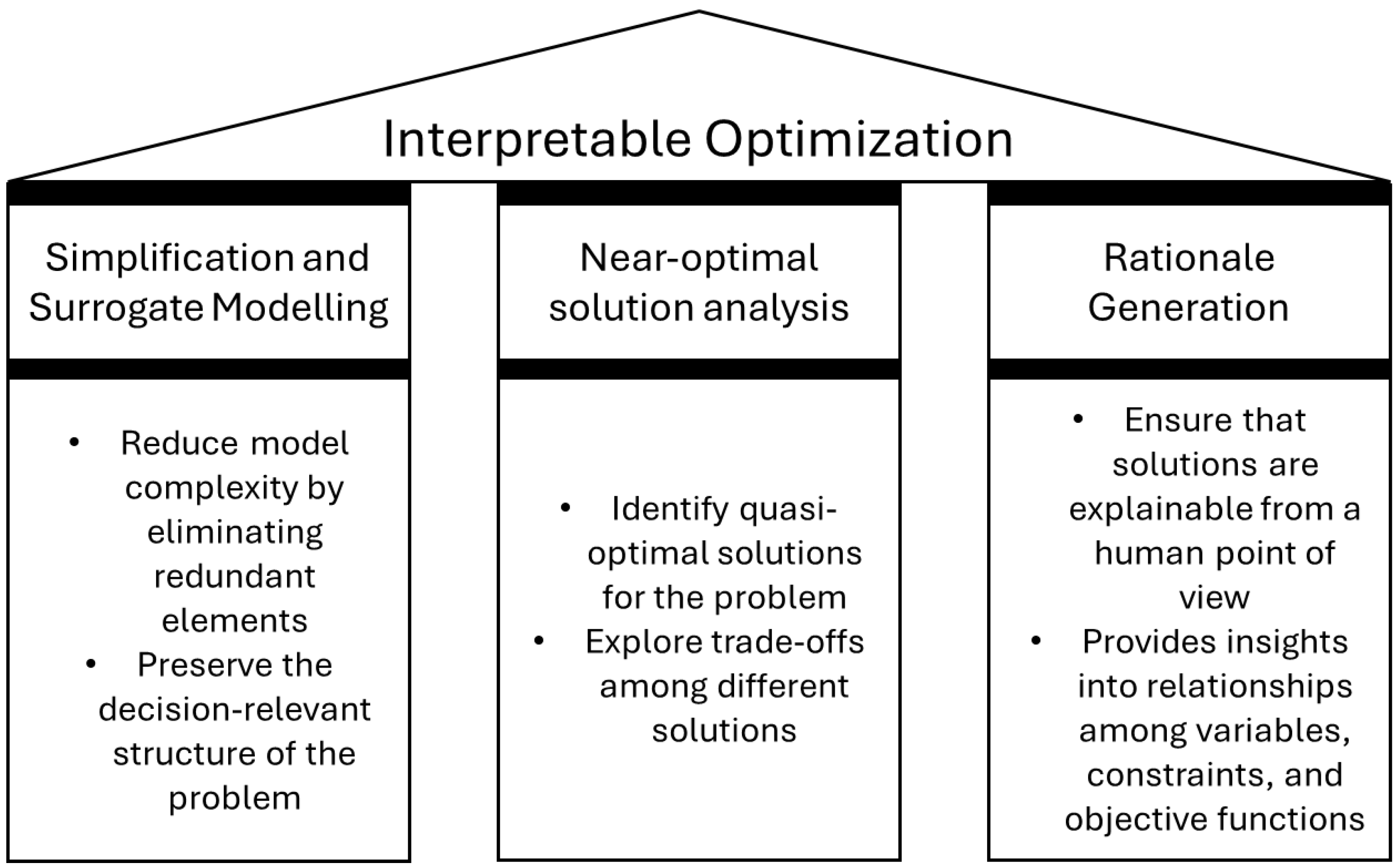
Our approach goes beyond these metrics by proposing several pillars or dimensions where interpretability metrics can be subsequently applied. We have identified three such pillars, which are shown in Figure 2 and will be reviewed in the remaining sections of this article.
The first pillar—simplification and surrogate model building—involves identifying the key variables, constraints, and relationships among them that define an optimization problem, while preserving its structural integrity. Traditional problem simplification techniques have aimed to improve computational efficiency by removing superfluous constraints and extraneous variables without explicitly considering interpretability. In contrast, interpretable optimization seeks to create simplifications that maintain decision-relevant information while making models easier to understand, even if some accuracy is lost in the process. These interpretable surrogates will serve as a complement to the initial problem rather than as a substitute, where the most important elements of the formulation, as well as their relationships, are extracted and presented. This means that, in the case of classical optimization, the formulation of the problem serves as the gold-standard definition of the decision, and every aspect highlighted in the surrogate model will be linked back to this original formulation.
The second pillar—near-optimal solution analysis—focuses on mapping the landscape of acceptable solutions, providing decision-makers with alternatives that are almost as good as the optimal solution. Many real-world optimization problems exhibit degeneracy, meaning multiple solutions yield similar objective values but with different trade-offs. Traditional optimization frameworks often emphasize finding a single optimal solution, overlooking the broader decision space. Metaheuristics, on the other hand, have been more cautious about the issues surrounding near-optimal solutions and have often made a point of returning not only one but a set of attractive alternatives. By analyzing near-optimal alternatives, interpretable optimization enables decision-makers to choose solutions that align with contextual priorities, constraints, and stakeholder preferences. In addition, the analysis of near-optimal solutions involves creating a perspective on the fitness landscape of the problem, which will inevitably be linked to the structure of solutions.
The third pillar—Rationale generation—addresses the fundamental challenge of explaining optimization outcomes. Instead of presenting an optimal decision as a purely mathematical result, interpretable optimization seeks to generate formal explanations for why a particular solution was selected. This involves linking decision variables to constraints and objectives, identifying causal relationships, and clearly articulating trade-offs. While methods such as dual variables and shadow prices provide limited insights on which resources are valuable and the general effect of constraints, interpretable optimization should aim to develop more comprehensive explanatory frameworks that improve trust and facilitate better decision-making, including generating rationales in natural language, which are easily understandable not only by modeling experts but also by stakeholders.
The remainder of this paper is devoted to presenting the initial work that has emerged in these three pillars. Then, we discuss real-world applications and future research directions, demonstrating the potential impact of interpretable optimization across various domains.

3. Problem Reduction and Surrogate Model Building

As explained, one of the cornerstones of interpretability is simplicity. There is a limit to the maximum number of elements the human mind can comprehend. Therefore, it is imperative to distill the most critical aspects of the optimization problem in order to create explanations that are understandable for a human being. This is why problem reduction is a cornerstone of interpretable optimization.

3.1. Can Problem Reductions Be Meaningful?

The possibility of obtaining interesting insights from simplification depends on the structure of the problem—if there is any structure in it at all. If eliminating even one of the most superficial elements leads to a completely different outcome, there would be no hope for interpretability. Fortunately, real-world optimization problems exhibit an inherent structure that enables simplification without a significant loss of accuracy [30].
This is exemplified by the Pareto principle [31], which suggests that, in most real-world cases, a small fraction of inputs often explains most of the variance in a system. If this principle holds for optimization problems, then structured reductions can preserve most of the decision-relevant information while improving transparency. Interpretable surrogates can then be built based on the extracted elements; even if they do not lead to the same optimal solutions, they can be used as a complement to build comprehensible explanations that can guide and support the decision process.
This is confirmed by empirical observations across multiple domains, where only a small subset of variables and constraints tends to drive decision outcomes. In power systems planning, for instance, large-scale transmission expansion problems often contain thousands of constraints, but only a handful of them critically influence the final investment decisions [32]. Similarly, in portfolio optimization, a small subset of risk factors typically dominates asset allocation decisions, allowing for simplified models that retain most of the original problem’s predictive power [33]. The structure hypothesis suggests that interpretable optimization can significantly reduce model complexity while preserving the essential characteristics of the decision problem.
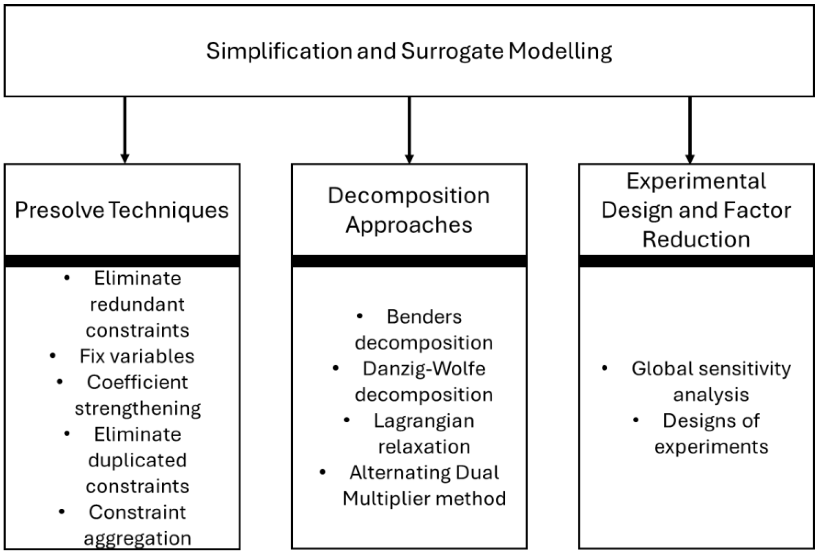
A long stream of literature has already addressed building simplified optimization problems, primarily to reduce computational complexity without sacrificing accuracy, rather than to improve interpretability. These methods are shown in Figure 3, and they will be discussed in the remainder of this section.

3.2. Presolve Techniques

Presolve techniques are applied as a previous step to any optimization, focusing on reducing problem size by eliminating redundant constraints and extraneous variables or strengthening constraints before solving the problem [34]. These methods can dramatically reduce computation time by modifying the original problem structure.
The main technique that has been applied to reduce problem size in linear and mixed-integer programming is presolving [35]. Presolve techniques can be categorized based on the type of simplification they introduce, as follows:
  • Eliminating redundant constraints: Constraints that do not impact the feasible region can be removed without affecting the optimal solution. This is particularly useful in large-scale problems where constraints may have been introduced for generality but are not binding in practice. Many different alternative strategies exist to prioritize constraints. For instance, in [36], several metrics were used to rank constraints by how likely they were to be bound. These metrics included the angle that the constraint formed with respect to the objective function, or how far some bounds of the left-hand side were from the right-hand side of the constraint (i.e., how far a constraint was from being bound).
  • Fixing variables: If the bounds of a variable force it to take a single value, that variable can be removed from the model, effectively turning it into a constant. This occurs in highly constrained problems where the interaction of multiple constraints results in a fixed solution for some variables. For example, in energy systems planning, transmission line constraints may fix the operational status of certain infrastructure components, making explicit modeling unnecessary [32].
  • Coefficient strengthening: If a constraint coefficient can be tightened without changing the feasible region, it enhances numerical stability and interpretability. This method is particularly useful in logistics and scheduling problems, where resource constraints can be reformulated for clarity [35].
  • Detecting and eliminating dominated constraints: Some constraints are made redundant by stronger constraints that enforce the same restrictions more effectively. Identifying and removing these constraints reduces problem size and eliminates unnecessary complexity in decision analysis.
  • Constraint aggregation: Certain sets of constraints can be combined into a single constraint, reducing the overall number of constraints while preserving the problem’s structure. This technique is commonly used in supply chain management and network flow problems to consolidate redundant constraints. For instance, identifying such umbrella constraints is key in problems such as a security-constrained power flow, where a planning solution must consider an unmanageably large number of constraints describing potential failures [37].
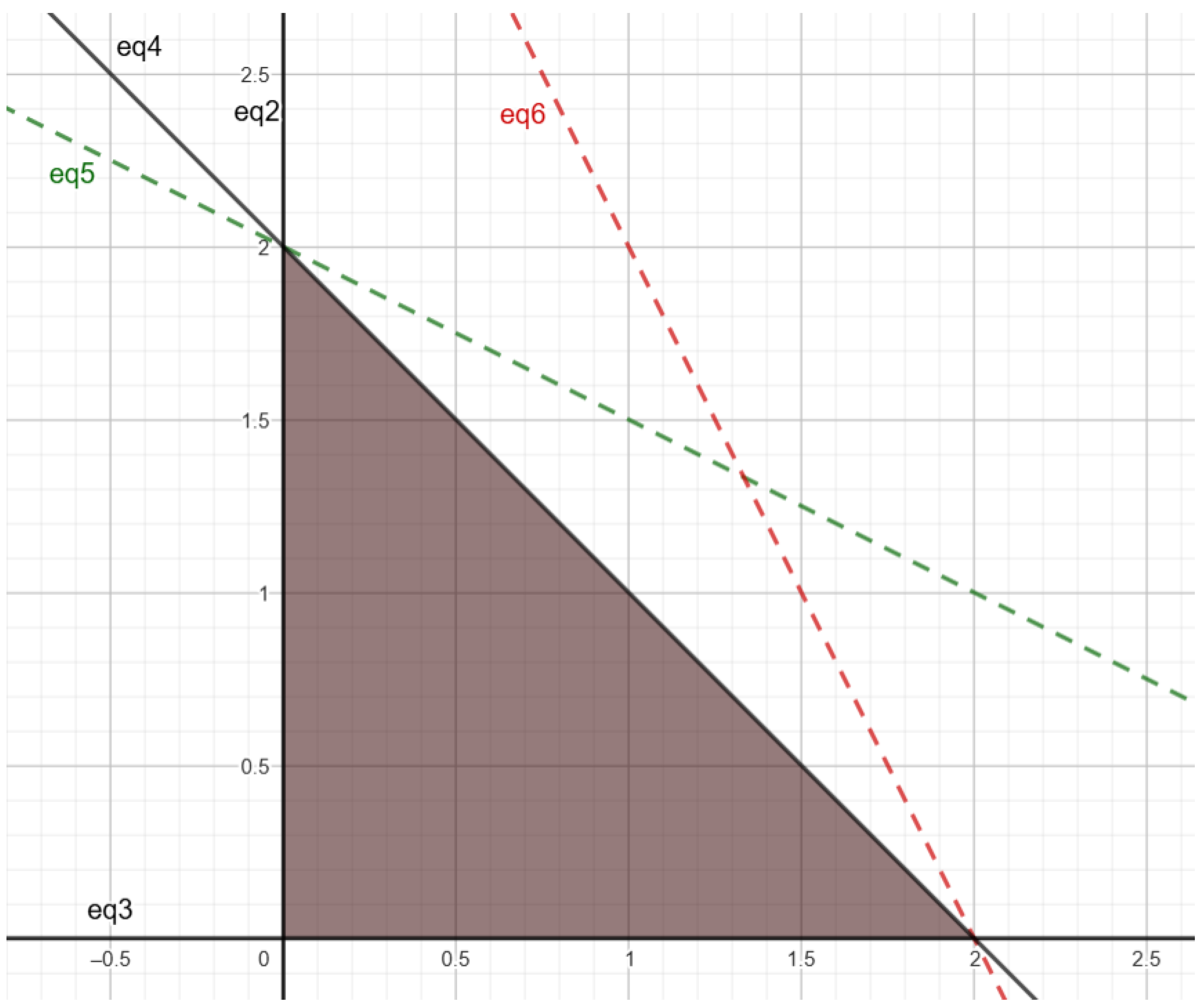
Let us consider the following optimization problem as an example of presolve methods:
min (3x + 2y)
x ≥ 0
y ≥ 0
x + y ≤ 2
x + 2y ≤ 4
2 x + y 4
Equation (1) defines the objective function of the optimization problem, and Equations (2)–(6) define the feasible region of the problem. Figure 4 shows a plot of the feasible region. The plot indicates that Equations (2)–(4) are enough to define the feasible region, while Equations (5) and (6) are redundant.
Presolve methods would figure out which equations are indeed necessary to define the feasible region (i.e., those equations that change the feasible region if removed from the problem) and which ones are redundant. They would then proceed to eliminate the latter equations before attempting to solve the problem.
The main advantage of presolve techniques is that most solvers automatically incorporate them, so a practical implementation is straightforward, and the problem solver does not need to implement them from scratch. Commercial solvers such as CPLEX, Gurobi, and Xpress have strong presolve capabilities that automatically perform variable-fixing, eliminate dominated and redundant constraints, aggregate constraints to reduce the problem size, and tighten variable bounds, potentially fixing their value [38,39,40]. Other open access solvers—such as SCIP, CBC, HiGHS, and GLPK—also include presolve functionalities, but they may lag behind the above-mentioned commercial solvers.
While presolve techniques may enhance the interpretability of optimization models by improving simplicity, they also introduce several challenges. The primary issue is the loss of the original formulation, as removing redundant constraints and fixing variables can obscure the initial problem structure, making it harder to explain how the simplified model relates to the original decision problem.
Several studies have shown the importance of presolve techniques. Achterberg et al. [34] performed a presolve analysis of MIP problems with Gurobi and showed that around 500 models out of a set of approximately 3000 were unsolvable when the presolve was disabled. For the remaining models, the presolve reduced the computation time needed by a factor of approximately nine. Achterberg and Wunderling [41] performed a presolve analysis of MIP problems with CPLEX, reaching similar conclusions.
To the best of our knowledge, the literature does not include a detailed benchmark of presolve capabilities among different solvers, but there are performance comparisons in terms of computation time when solving problems, and commercial solvers tend to outperform the open access ones [42].

3.3. Decomposition Approaches

Another traditional approach that has been applied to problem simplification is decomposition. Decomposition techniques in optimization break down complex problems into smaller, more manageable subproblems that can be solved independently or iteratively coordinated to find an optimal solution. These methods are particularly useful for large-scale optimization problems, where solving the entire model directly would be computationally prohibitive.
One widely used approach is Benders’ decomposition [43], which separates decision variables into master problem and subproblems, iteratively refining feasibility and optimality cuts to converge to the optimal solution.
Benders’ decomposition solves large-scale optimization problems by partitioning them into a master problem and a subproblem, both of which are solved iteratively. The master retains the complicating (typically integer, aggregate, or investment) variables, while the subproblem optimizes the remaining continuous variables, conditional on the master’s current solution. The subproblem returns either an optimal objective value or feasibility/optimality cuts—linear constraints that summarize its outcome—which are appended to the master. Subproblems are independent and can be solved in parallel. This exchange continues until no further cuts arise, at which point the master’s solution is provably optimal for the original problem. Benders’ decomposition can be applied to a very large scope of problems, namely two-stage stochastic ones, where complicating variables correspond to investment decisions taken in the first stage, and the non-complicating ones are the second-stage decisions that affect only one particular scenario [44]. Benders’ decouples the investment and operation decisions and provides an economic value for the second stage (the recourse function), facilitating the potential interpretation of solutions. The main disadvantage of Benders’ decomposition is its slow convergence [45]. Many Benders’ cuts may be necessary until the algorithm converges, and each iteration requires solving an additional master problem and subproblems, which may be computationally intensive [46].
Another key technique is Dantzig–Wolfe decomposition [47], which reformulates a large problem into a master problem and subproblems based on a column-generation approach, improving efficiency in structured linear programs. The main strength of Danzig–Wolfe decomposition is that the subproblems are independent, enabling parallelization [48]. Its main weakness is that, under some circumstances, convergence is not guaranteed and may not be reached [49].
Lagrangian relaxation [50] is also commonly used, where complicating constraints are relaxed and incorporated into the objective function through Lagrange multipliers, allowing the problem to be solved as a series of simpler subproblems. Its main advantage lies in its ability to handle complicated constraints [51], and the main disadvantage is that the solution of the relaxed problem may be unfeasible in the original problem [52].
Additionally, the Alternating Dual Multiplier Method (ADMM) is an iterative decomposition approach that updates dual multipliers in an alternating fashion to optimize separable convex problems efficiently [53]. ADMM is particularly effective in distributed optimization and large-scale convex programming, enabling parallel computation while maintaining convergence properties. Its main strength is that parallelization allows for application in large-scale problems [54], while its main weakness is that convergence is only guaranteed if the problem is convex [55].
The scalability of decomposition methods is fundamentally influenced by the structure of the constraint matrix, particularly the extent to which it permits decomposition into loosely coupled subcomponents. Benders’ decomposition is well suited for problems exhibiting a clear division between complicating and non-complicating variables, often reflected in a constraint matrix where a small set of linking constraints connects otherwise independent blocks. It scales effectively by iteratively solving a relatively small master problem alongside multiple parallelizable subproblems, although performance may degrade as the number of Benders’ cuts increases. Dantzig–Wolfe decomposition is the most efficient for problems with a block-angular constraint matrix, wherein several independent submatrices are coupled through a limited set of global constraints. This structure facilitates scalable column generation, making the method particularly appropriate for large-scale linear programs. Lagrangian relaxation achieves strong scalability when the coupling constraints are dualized, yielding fully separable subproblems that may be solved in parallel. However, its reliance on dual optimization may result in slow convergence and solutions that are not feasible in the primal space. ADMM is highly scalable in large convex optimization problems where the constraint structure supports variable splitting or consensus formulations. In such cases, subproblems can be solved independently, with coordination achieved through simple consistency constraints, making ADMM particularly effective for distributed and parallel computing environments.
Table 1 summarizes the decomposition methods mentioned in this section. Each method is particularly well suited for a different type of problem structure.
These decomposition methods are essential for solving large-scale linear, mixed-integer, and nonlinear optimization problems, particularly in logistics, energy systems, and network design. Unfortunately, these decomposition approaches may obscure interpretability, as they obscure the original formulation. In Benders’ decomposition, the fact that cuts describe the recourse function can be repurposed to provide an interpretation of the consequences of first-stage (or complicating) decisions. However, the potential for interpretability in Dantzig–Wolfe decomposition is lower, as the variables are introduced sequentially and the link between them and the initial problem statement is obscured. On the contrary, Lagrangean Relaxation can simplify the problem, and dual multipliers can provide interesting insights for interpretation. Finally, ADMM also has an interesting interpretability potential in its decomposition of the problem. However, as explained above, in virtually all applications, the focus of stochastic decomposition techniques is efficiency rather than interpretability, and additional research should focus on tailoring these techniques to improve the explainability of optimization results.

3.4. Experimental Design and Factor Reduction

Factor reduction methods are crucial in experimental design for simplifying complex models while retaining the most significant factors. We will interpret factors as any relevant element of the problem (i.e., variables, constraints, or parameters) in the context of optimization problems. These techniques have been applied to models in many contexts to improve computational efficiency, enhance interpretability, and support decision-making, as they identify and remove factors with minimal impact on system performance.
Various approaches exist, each suited to different problem structures and objectives. One common approach is Global Sensitivity Analysis (GSA), where methods like the Morris method systematically perturb input factors to assess their influence on model outputs [56]. Morris distinguishes between the important, interactive, and insignificant variables by computing the elementary effects. This distinction is the main takeaway from its application, rather than the specific result value (this is why some authors refer to it as a qualitative method). Important variables are those with a significant impact on the model’s output, interactive variables that exhibit non-linear interactions, while insignificant variables contribute minimally to system performance and can be candidates for removal. In addition, the fact that the method is built on calculating a sample of one-at-a-time perturbations can cause the results to depend on calculation order, making them unstable if there is nonlinearity [56,57].
Several improvements have been proposed to refine the Morris method. Menberg et al. [58] introduced using the median instead of the mean for ranking parameters, making sensitivity assessments more robust against outliers. Ge and Menendez [59] adapted the method for models with dependent inputs, resulting in more accurate sensitivity estimates for correlated systems. Li et al. [60] combined the Morris method with a sequential sampling strategy to improve the coverage of the input space and enhance sensitivity estimation. Ţene et al. [61] incorporated copula-based dependency structures for interactions between model parameters, making the method more suitable for complex systems with interrelated variables. Another extension, the controlled Morris method by [62,63], introduced a sequential testing procedure that enhances factor screening without requiring predefined distributions. GSA has arguably not found extensive application due to its very intensive computational requirements. However, recent advances in computational capacity have motivated a renaissance in applications [64].
Design of Experiments (DOE) techniques offer another approach to factor reduction by structuring experiments efficiently. One avenue to reduce the number of necessary experiments is to perform only a fraction of factor combinations (Fractional Factorial Design). Fractional Factorial Design includes the Taguchi method [65], which uses orthogonal arrays to systematically vary input factors while minimizing the number of required experiments. This can efficiently increase the signal-to-noise ratio of experiments; however, this comes as a cost. Some of the interactions are ignored or aliased, so they will not be identified by this technique. Sequential analysis [66] structures experiments sequentially to avoid sampling where more information is not required. This is extremely useful when experiments are expensive, as it allows for the flexible introduction of new information as more problem features are discovered. Complementarily, if the problem structure is known, optimal design [67] allows parameters to be estimated without bias and with minimum variance. A non-optimal design requires more experimental runs, leading to higher computational costs.
Table 2 shows a comparison among the methods described in this subsection, highlighting their main strengths and weaknesses, as well as pointing out problems where they are particularly well suited.
The Morris method, Taguchi method, sequential analysis, and optimal design represent distinct strategies within experimental design and analysis, each tailored to different goals and contexts. The Morris method is a GSA technique ideal for computational models with many input variables, primarily used for early-stage screening to identify influential factors. In contrast, the Taguchi method focuses on improving process robustness and reducing variation by using orthogonal arrays and maximizing signal-to-noise ratios, making it well suited for quality engineering in industrial settings. Sequential analysis differs fundamentally as it enables data-driven decisions during experimentation, allowing trials to be stopped early based on accumulated evidence—an approach particularly valuable in clinical trials. Finally, optimal design methods, such as D-optimal or A-optimal designs, aim to maximize the statistical efficiency of parameter estimation by strategically selecting design points based on model structure. While all four methods serve experimental purposes, they vary significantly in statistical rigor, adaptability, and application domains—from qualitative screening and robust quality control to dynamic decision-making and precision modeling. While these techniques have been widely adopted in statistical modeling, their application to mathematical optimization remains underexplored. The challenge is to adapt these principles to identify decision-relevant variables and constraints, ensuring that the simplified model remains faithful to the original problem’s structure.
To address these challenges, there is a need for simplification and surrogate model methods that explicitly preserve decision-relevant structures rather than solely focusing on computational efficiency.

4. Analysis of Near-Optimal Solutions

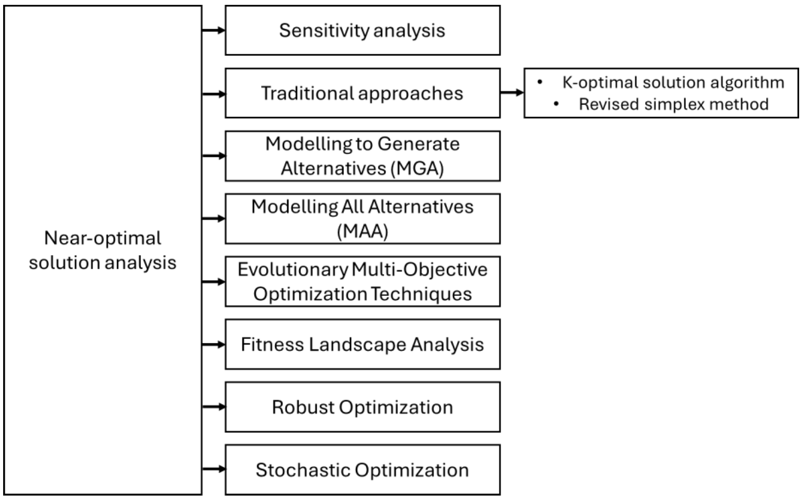
This section describes the second pillar of the framework introduced in Section 2.3, which is related to the study of near-optimal solutions in optimization problems. Figure 5 shows the methods and techniques that will be described in the remainder of this section.

4.1. A Degenerate Class of Problems

Mathematical optimization is traditionally aimed at finding a single optimal solution that either minimizes or maximizes an objective function while adhering to a set of constraints. However, real-world optimization problems commonly exhibit multiple quasi-optimal solutions, meaning that different configurations can lead to nearly identical outcomes. This phenomenon is evident across numerous domains, aligning with findings in combinatorial optimization, where solution spaces frequently contain clusters of similarly effective solutions [23].
For example, different network expansion strategies in power systems may yield comparable cost and reliability metrics despite involving distinct infrastructure investments [76]. Likewise, in healthcare resource allocation, varying bed capacity expansion strategies can lead to similar patient outcomes, offering greater flexibility in decision-making [10]. This suggests that decision-makers should not be restricted to a single recommendation but instead consider a spectrum of viable alternatives—which we will refer to as quasi-optimal alternatives (QOAs)—that are near-optimal or quasi-optimal solutions, defined as a set of solutions that remain close to the optimal one within a specified tolerance [77].

4.2. Sensitivity Analysis

Traditional sensitivity analyses and scenario testing offer only a limited perspective on this space, as they focus on perturbations around a single solution rather than mapping the broader landscape of alternatives [78]. Sensitivity analysis makes it possible to find other quasi-optimal solutions with a structure where only one of the variables is altered. However, explicitly characterizing QOAs enables decision-makers to explore alternative solutions that align more closely with qualitative considerations, such as policy constraints, ethical guidelines, or stakeholder preferences [79].

4.3. Traditional Approaches

The exploration of near-optimal spaces has been widely applied in the field of chemical engineering, particularly in capacity expansion problems (also known as “synthesis” problems) [80]. Arguably, the first technique applied to obtain near-optimal solutions was the K-optimal solutions algorithm [81], in which the optimal solution is excluded from the problem, and the problem is re-run with an additional constraint requiring the solution to be within a small distance in terms of the objective function (e.g., 5%). This process is repeated k times to find k different near-optimal solutions. The revised simplex method [82] can obtain these solutions more efficiently in the case of linear programming. Most researchers exploring near-optimal spaces focus on computing numerous near-optimal solutions from which they derive insights [83].

4.4. Model Generating Alternatives and Mapping All Alternatives

In the 1980s, Modeling to Generate Alternatives (MGA) was introduced [84], where the K-optimal solutions problem is modified to maximize the distance between the optimal and target solutions according to several search directions. This maps the most extreme solutions that are still near optimal. MGA has recently been applied to energy systems [80,85,86,87]. However, the solutions found by MGA might not be the most interesting ones, as they represent the extremes of the near-optimal space.
Another technique, known as Modeling All Alternatives, discretizes the whole space and explores it to identify common elements [86,88,89]. The latter reference introduces the idea of identifying the Chebyshev center of the near-optimal solution space (the one farthest away from its defining convex hull).
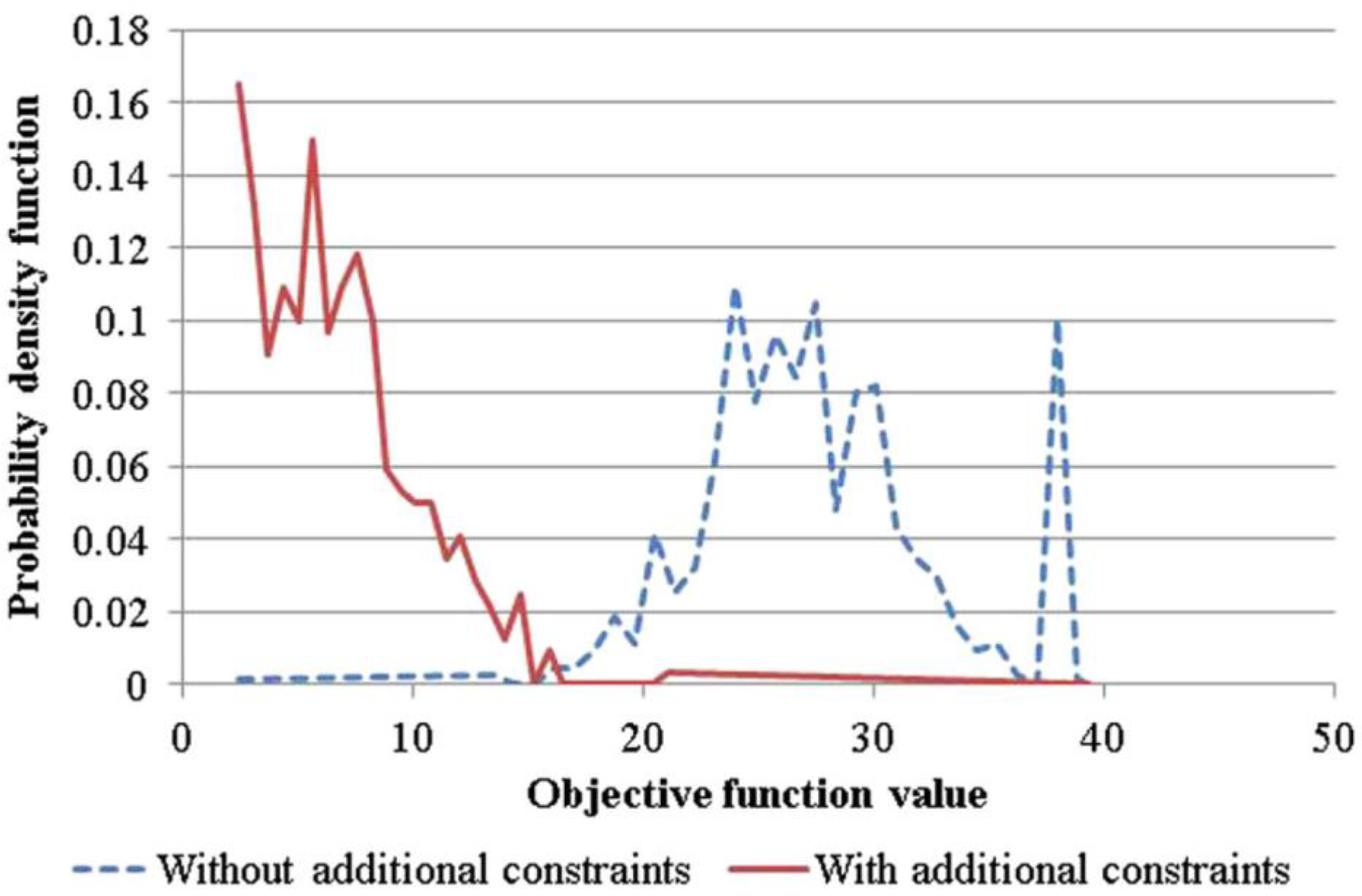
Dubois and Ernst have gone one step further, identifying the necessary conditions for optimality as the common elements that all near-optimal solutions share [90]. Lumbreras et al. [91] also proposed this search for common elements in the pre-run of the optimization to reduce the solution time of a network optimization problem by several orders of magnitude. In Figure 6, two probability distributions for the objective value of general solutions and near-optimal solutions (defined through additional constraints) can be seen, highlighting how much better the latter can be.

4.5. QOAs in Evolutionary Computation

Modern heuristic and evolutionary optimization algorithms increasingly incorporate mechanisms to explore diverse near-optimal solutions. Evolutionary multi-objective optimization techniques [92] are particularly relevant in this context, as they generate a Pareto front of solutions that balance competing objectives. These methods enhance decision-making by illuminating the trade-offs between criteria and improving interpretability.
Fitness landscape analysis offers another valuable perspective by examining the structural properties of the solution space, identifying clusters of near-optimal solutions, and analyzing their interconnections [93]. A deeper understanding of the topology of near-optimal solutions allows decision-makers to select alternatives that are not only optimal but also resilient to external perturbations.

4.6. Other Approaches That Are Related but Do Not Directly Correspond to This Pillar

Robust optimization in problems subject to uncertainty seeks solutions that maintain near-optimal performance in various scenarios rather than optimizing for a single expected scenario [94]. Stochastic programming further extends this concept by incorporating probability distributions to determine the best decision across multiple uncertain outcomes [95]. However, it should be noted that these approaches do not output a set of near-optimal solutions, which is the key expected result of this pillar. They result in one single solution, which remains feasible across all scenarios in the case of robust optimization, and which has the best expected value in the case of stochastic optimization.
Table 3 shows the methods for analyzing the near-optimal solutions discussed in this section, highlighting their main strengths and weaknesses.

4.7. A Need to Integrate Optimization

Finding near-optimal solutions involves several significant challenges that must be carefully addressed to enhance their practical value in decision-making. One of the foremost difficulties lies in defining meaningful diversity [109]. Merely identifying different solutions is not enough; decision-makers require alternatives that vary significantly in terms of constraints, decision variables, and trade-offs. While techniques like MGA have been designed to enforce structural diversity, their integration into standard optimization frameworks—in a way that exploits problem structure rather than blindly solving multiple problem instances—remains an ongoing research endeavor [84].
Another major hurdle is the effective visualization and interpretation of near-optimal solutions. Decision-makers often struggle to extract actionable insights from large sets of solutions, particularly when trade-offs are complex and multidimensional. To enhance interpretability, decision maps, heatmaps, and clustering-based categorization can provide more intuitive representations of alternative solutions [110]. However, despite their potential, these tools must be further refined to ensure usability across a broad range of applications.
One particular issue is that the QOAs should be expressed in terms that experts would understand, which some authors have referred to as “meta-solutions” [18]. The automatic definition of these meta-solutions as a function of their features is a challenge, as it is usually assumed that it is only through experts that this definition can be found.
The next section introduces the advances made in generating solution rationales, corresponding to the third pillar of the proposed framework, and builds on the previous developments.

5. Generating Solution Rationales

While it is possible to explain how an optimization model generates a solution—through mathematical formulation, solvers, and optimality conditions—this explanation is often inaccessible to non-experts. The real challenge lies in explaining why a particular solution is chosen over another at a given moment [111,112].
For example, while the model’s mechanics can be described, it remains difficult to justify to a worker why today’s production plan follows type A while yesterday’s followed type B. If workers cannot understand the reasoning behind such decisions, they may struggle to anticipate future outcomes, such as overtime requirements or weekend shifts, leading to dissatisfaction, resistance, or inefficiencies.
Without comprehensible justifications, users may perceive optimization systems as black boxes, reducing trust and hindering their adoption. Effective decision support should prioritize explanations over technical details, ensuring that end users can relate decisions to their own operational context and expectations, ultimately improving both compliance and efficiency.
The generation of solution rationales builds on the simplifications and the landscape of QOAs to build structured explanations that articulate the reasoning behind an optimization decision. These explanations can then be translated into natural language using NLP-based techniques, making them accessible to a broader audience. The explanations should be based on the following elements of the problem: important variables, binding constraints, and tradeoffs. The concept of a tradeoff itself should be adapted from that of multicriteria decision methods, as explanatory tradeoffs can occur even in the same objective function through its subcomponents.
For instance, performing plan A first might be better for the sale of product X and worse for the sale of product Y. If product X is more important, we can explain a change in the production plans. By structuring explanations in this way, we ensure that the rationale behind an optimization decision is both mathematically sound and interpretable by non-experts. We refer the reader back to Section 1.2 for more information on the state of the art in these techniques.

6. Example Applications

This section presents two examples of fields that would benefit from the application of interpretable optimization. They should be understood merely as an illustration of its potential, as future developments may lead to unexpected applications in a myriad of fields where optimization already plays a strong role in the decision-making process.

6.1. Energy Systems and Carbon Emission Reduction

Policymakers and stakeholders in the energy sector must plan long-term infrastructure while balancing economic, environmental, and social objectives. Interpretability is critical in this context, as energy transition plans affect millions of households and require public approval. Investors and policymakers need clear explanations of why specific energy pathways were chosen over others, and grid operators and industry stakeholders require interpretable solutions to manage the trade-offs between cost, reliability, and sustainability.
Failing to provide clear explanations may lead to hurdles when planned decisions move into the implementation phase. The SuedLink transmission line project in Germany—crucial for distributing wind energy from the north to the south—has experienced considerable delays. Local communities and environmental groups have opposed the project, raising concerns over landscape disruption, impacts on property values, and perceived health risks from electromagnetic fields [113].
Similarly, proposed wind farms in Italy’s Apennine Mountains have faced resistance due to concerns over natural habitat destruction, noise pollution, and visual impacts on significant landscapes, resulting in necessary assessments, negotiations, and project redesigns, which have delayed the planning-to-operation timeline.
In the UK, the Navitus Bay Wind Park, intended to power approximately 700k homes, was canceled due to concerns over potential harm to tourism, marine life, and the site’s natural beauty [114]. Guan and Zepp [115] studied several factors influencing the community acceptance of onshore wind farms in Eastern China, showing that insufficient information dissemination was the most significant factor regarding acceptance.
These examples showcase several issues that are making energy planning increasingly difficult. Stakeholder consensus is key but becoming more difficult to achieve, and, equally important, it is necessary to always plan with alternatives. Different plans can be very similarly effective in terms of their primary outcomes, yet they can have divergent implications, such as in terms of their landscape impact.
Potential issues in the implementation phase could be mitigated by providing a sensitivity analysis, in which the influence of parameters is studied to enhance the interpretability of the results.

6.2. Ethical Policy Spending and Fair Budget Allocation

Governments must allocate public funds by balancing competing demands from various stakeholders in healthcare, education, infrastructure, and social programs. Non-governmental organizations face similar challenges, weighing the needs of several stakeholders with different priorities [116].
Stakeholders use influence strategies to exert pressure and achieve their goals [117]. Interpretability is crucial to ensuring that budget decisions are transparent, equitable, and justifiable. Public trust and policy effectiveness depend on the involvement of citizens in the budgeting process [118], which can be fostered by clear explanations of why certain funding priorities were chosen over others. Legal mandates, regional inequalities, and economic impact are among the critical constraints shaping budget distribution, making it essential to explore alternative allocations that maintain efficiency and fairness.
Transparency in budgetary decisions yields benefits such as reducing the unused budget, a metric that measures budget inefficiency [119]. Farazmand et al. [120] demonstrated that transparency and accountability in budgetary decisions are particularly relevant under critical situations, such as the COVID-19 pandemic. Transparency would avoid undesirable biases, which have led to scandals such as the Dutch case, where dual citizens were subjected to stricter scrutiny when evaluating possible fraud in childcare benefit claims [121].

6.3. Healthcare

There are several problems related to healthcare where the application of optimization models can be advantageous. Such problems include (among others) resource allocation, organ allocation, treatment planning, disease management, personnel planning, patient scheduling, and facility location [122].
Digitalization technologies record and store massive volumes of historical data. Computerized models can help make the most of the data, distilling insights that would have been missed otherwise. Such models could be directly integrated into healthcare systems, and they have already proven their effectiveness in handling large datasets and providing useful practical results [123].
Optimization models can provide useful assistance, but they cannot fully replace human intervention. Interactions between people and computerized systems are critical in clinical decisions, and it is crucial to involve patients in the decision-making processes [124]. Similarly, human insights and personal preferences are also fundamental in decisions concerning hospital management [125].
Understanding the logic behind the results that a computer provides is especially important in decisions where the lives of patients could be at stake. Under such circumstances, it is difficult to trust black-box procedures whose logic goes beyond human capabilities, and fostering the development of interpretable optimization could provide tremendously valuable tools.
The analysis of near-optimal solutions, along with the generation of rationale that explains why these solutions were selected from a human point of view, would provide a set of solutions where each alternative includes an explanation that people can understand. These explanations would provide people with a solid foundation on which they could base their decisions.

7. Conclusions: The Road Ahead

Interpretable optimization is an emerging field that addresses a crucial gap between mathematical optimization and real-world decision-making. While interpretability has gained significant attention in machine learning, optimization models often remain completely opaque, limiting their adoption and trustworthiness. The ability to understand and justify optimization decisions is essential, particularly in high-stakes applications such as energy planning, healthcare, and resource allocation.
Without transparency, stakeholders may struggle to assess the reliability of model outputs, leading to resistance to implementation or unintended biases in decision-making. Ensuring that optimization-driven decisions align with ethical and legal standards is key. Unlike black-box machine learning models, classical optimization inherently possesses a degree of transparency due to its explicit mathematical formulation. However, the link between a model’s structure and its final solution is often unclear, necessitating enhancements in interpretability.
This paper introduces a framework for interpretable optimization that builds upon the following three key pillars: simplification and surrogate modeling to retain decision-relevant structures, near-optimal solution analysis to provide competitive alternatives, and rationale generation to ensure that solutions are explainable and actionable. Each of these elements contributes to making optimization models not only computationally efficient but also accessible to decision-makers.
The first pillar of the framework is simplification and surrogate modeling. One of the major challenges in optimization lies in its complexity. Large-scale problems often require reduction techniques, such as presolving and decomposition, to improve computational feasibility and efficiency. However, these methods can sometimes obscure the original problem structure, reducing interpretability. For example, presolve techniques can distinguish between directly eliminating constraints whose removal does not affect the feasible region of the optimization problem—such as eliminating duplicated constraints—and other techniques that may affect the interpretability of the solutions, such as aggregating several constraints into a single one.
Presolve and decomposition techniques can serve as a starting point to derive specific interpretation-driven methods that simplify the problem in a meaningful manner. For instance, the recourse function defined as a function of key variables in Benders’ decomposition, the dual multipliers in Lagrangean relaxation, or the subproblems in ADMM all present very interesting potentials that could be exploited in methods tailored for this purpose.
In addition, techniques such as sensitivity analysis, the Morris method, and Design of Experiments in general can help prioritize relevant factors, improving the clarity of optimization models while maintaining their decision-making utility. This can also be used as a stepping stone in the development of interpretable surrogates focused on factors that are not only relevant in terms of their impact but also closely linked to the most intuitive variables and parameters of the problem.
The second pillar of the framework is near-optimal solution analysis. Techniques such as MGA and MAA provide ways to systematically identify diverse yet effective solutions. Evolutionary and heuristic approaches, as well as landscape fitness analysis, enhance this process by explicitly exploring subobjectives or providing a description of the entire solution space. However, there is a challenge in making these methods scalable for large problems, as well as in defining meaningful diversity among alternatives, ensuring that solutions are not only mathematically distinct but also practically relevant [109]. Future work should focus on integrating near-optimal analysis into standard optimization frameworks to improve usability in real-world decision-making.
The visualization of near-optimal solutions is another research area that demands attention. Decision-makers often struggle to evaluate trade-offs among solutions in large-scale problems that involve thousands of decision variables and constraints. Techniques focusing on dimension reduction, such as clustering, could help facilitate the visualization of these solutions.
The third pillar of the framework is rationale generation. Effective decision support must emphasize not only how a solution was computed but also why specific choices were made. Approaches such as counterfactual explanations, surrogate models, and feature-based descriptions can help bridge this gap, offering intuitive representations of optimization outputs in the form of understandable rules that facilitate stakeholder engagement and trust. These approaches should be integrated into optimization frameworks in a rigorous manner so that they can be used efficiently across a wide range of problems.
In the literature, few examples aim to generate solution rationales that explain why a specific solution was selected in a way that is easily comprehensible. These examples are tailored to specific problems, and their methods and techniques should be generalized so that they can be applied to a broader set of problems.
The future of interpretable optimization lies in balancing mathematical rigor with human-centered insight. As optimization models grow in complexity, making their decisions understandable is not just a technical challenge but a necessity. Transparency enhances efficiency by allowing decision-makers to confidently leverage optimization insights, reducing implementation resistance and improving real-world applicability. At the same time, interpretability is a fundamental ethical imperative, ensuring that automated decisions remain fair, accountable, and aligned with societal values. Bridging this gap between efficiency and ethics is crucial for the responsible deployment of optimization in critical sectors, shaping a future where data-driven decision-making is both powerful and just.

Author Contributions

Conceptualization, S.L.; Investigation, S.L. and P.C.; Writing—original draft, S.L. and P.C.; Writing—review & editing, S.L. and P.C.; Visualization, S.L. and P.C.; Supervision, S.L.; All authors have read and agreed to the published version of the manuscript.

Funding

This research received no external funding.

Acknowledgments

The authors have used ChatGPT to refine some sections based on a specific outline provided by the authors, to improve the flow of some sections, and to gain insights from papers. A GPT tool with the “Elements of style” was used to improve style with minimal changes based on the rules of this book. Grammarly was used to improve grammar and to simplify some convoluted expressions. Elicit Pro and ChatGPT were used to complement classical search with Google Scholar and found several papers that would have otherwise been overlooked because of slightly different keywords and abstracts. The authors revised all these changes carefully and are responsible for the final version of the text.

Conflicts of Interest

The authors declare no conflict of interest.

References

  1. Rudin, C. Stop explaining black box machine learning models for high stakes decisions and use interpretable models instead. Nat. Mach. Intell. 2019, 1, 206–215. [Google Scholar] [CrossRef] [PubMed]
  2. Attard-Frost, B.; De los Ríos, A.; Walters, D.R. The ethics of AI business practices: A review of 47 AI ethics guidelines. AI Ethics 2023, 3, 389–406. [Google Scholar] [CrossRef]
  3. Washington, A.L. How to Argue with an Algorithm: Lessons from the COMPAS-ProPublica Debate. Color. Technol. Law. J. 2018, 17, 131. Available online: https://scholar.law.colorado.edu/ctlj/vol17/iss1/4 (accessed on 25 February 2025).
  4. Roscher, R.; Bohn, B.; Duarte, M.F.; Garcke, J. Explainable Machine Learning for Scientific Insights and Discoveries. IEEE Access 2020, 8, 42200–42216. [Google Scholar] [CrossRef]
  5. Mosca, E.; Szigeti, F.; Tragianni, S.; Gallagher, D.; Groh, G. SHAP-Based Explanation Methods: A Review for NLP Interpretability. In Proceedings of the 29th International Conference on Computational Linguistics, Gyeongju, Republic of Korea, 12–17 October 2022; Calzolari, N., Huang, C.-R., Kim, H., Pustejovsky, J., Wanner, L., Choi, K.-S., Ryu, P.-M., Chen, H.-H., Donatelli, L., Ji, H., et al., Eds.; International Committee on Computational Linguistics: Gyeongju, Republic of Korea, 2022; pp. 4593–4603. [Google Scholar]
  6. Antonini, A.S.; Tanzola, J.; Asiain, L.; Ferracutti, G.R.; Castro, S.M.; Bjerg, E.A.; Ganuza, M.L. Machine Learning model interpretability using SHAP values: Application to Igneous Rock Classification task. Appl. Comput. Geosci. 2024, 23, 100178. [Google Scholar] [CrossRef]
  7. Zafar, M.R.; Khan, N. Deterministic Local Interpretable Model-Agnostic Explanations for Stable Explainability. Mach. Learn. Knowl. Extr. 2021, 3, 525–541. [Google Scholar] [CrossRef]
  8. Pizarroso, J.; Portela, J.; Muñoz, A. NeuralSens: Sensitivity Analysis of Neural Networks. J. Stat. Softw. 2022, 102, 1–36. [Google Scholar] [CrossRef]
  9. Slack, D.; Hilgard, S.; Jia, E.; Singh, S.; Lakkaraju, H. Fooling LIME and SHAP: Adversarial Attacks on Post hoc Explanation Methods. In Proceedings of the AAAI/ACM Conference on AI, Ethics, and Society, Jose, CA, USA, 21–23 October 2024; ACM: New York, NY, USA, 2020; pp. 180–186. [Google Scholar]
  10. Izquierdo, J.L.; Ancochea, J.; Soriano, J.B. Clinical Characteristics and Prognostic Factors for Intensive Care Unit Admission of Patients With COVID-19: Retrospective Study Using Machine Learning and Natural Language Processing. J. Med. Internet Res. 2020, 22, e21801. [Google Scholar] [CrossRef]
  11. Bertsimas, D.; Pauphilet, J.; Van Parys, B. Sparse Regression: Scalable Algorithms and Empirical Performance. Stat. Sci. 2020, 35, 555–578. [Google Scholar] [CrossRef]
  12. Forel, A.; Parmentier, A.; Vidal, T. Explainable data-driven optimization: From context to decision and back again. In Proceedings of the 40th International Conference on Machine Learning, Honolulu, HI, USA, 23–29 July 2023; JMLR.org: Honolulu, HI, USA, 2023. [Google Scholar]
  13. Aigner, K.-M.; Goerigk, M.; Hartisch, M.; Liers, F.; Miehlich, A. A framework for data-driven explainability in mathematical optimization. In Proceedings of the Thirty-Eighth AAAI Conference on Artificial Intelligence and Thirty-Sixth Conference on Innovative Applications of Artificial Intelligence and Fourteenth Symposium on Educational Advances in Artificial Intelligence, Vancouver, BC, Canada, 20–27 February 2024; AAAI Press: Washington, DC, USA, 2024. [Google Scholar]
  14. Korikov, A.; Beck, J.C. Objective-Based Counterfactual Explanations for Linear Discrete Optimization. In Proceedings of the Integration of Constraint Programming, Artificial Intelligence, and Operations Research: 20th International Conference, CPAIOR 2023, Nice, France, 29 May–1 June 2023; Proceedings. Springer: Berlin/Heidelberg, Germany, 2023; pp. 18–34. [Google Scholar]
  15. Kurtz, J.; Birbil, Ş.İ.; Hertog, D.d. Counterfactual Explanations for Linear Optimization. arXiv 2024, arXiv:2405.15431. [Google Scholar] [CrossRef]
  16. Ciocan, D.F.; Mišić, V.V. Interpretable Optimal Stopping. Manag. Sci. 2022, 68, 1616–1638. [Google Scholar] [CrossRef]
  17. Čyras, K.; Letsios, D.; Misener, R.; Toni, F. Argumentation for Explainable Scheduling. Proc. AAAI Conf. Artif. Intell. 2019, 33, 2752–2759. [Google Scholar] [CrossRef]
  18. Goerigk, M.; Hartisch, M. A framework for inherently interpretable optimization models. Eur. J. Oper. Res. 2023, 310, 1312–1324. [Google Scholar] [CrossRef]
  19. Lumbreras, S.; Tejada, D.; Elechiguerra, D. Explaining the solutions of the unit commitment with interpretable machine learning. Int. J. Electr. Power Energy Syst. 2024, 160, 110106. [Google Scholar] [CrossRef]
  20. Amram, M.; Dunn, J.; Zhuo, Y.D. Optimal policy trees. Mach. Learn. 2022, 111, 2741–2768. [Google Scholar] [CrossRef]
  21. Bertsimas, D.; Dunn, J.; Mundru, N. Optimal prescriptive trees. Inf. J. Optim. 2019, 1, 164–183. [Google Scholar] [CrossRef]
  22. Wolsey, L.A.; Nemhauser, G.L. Integer and Combinatorial Optimization; John Wiley & Sons, Ltd.: Hoboken, NJ, USA, 1988; ISBN 978-0-471-82819-8. [Google Scholar]
  23. Papadimitriou, C.H.; Steiglitz, K. Combinatorial Optimization: Algorithms and Complexity; Dover Books on Computer Science; Dover Publications: Garden City, NY, USA, 1998; ISBN 978-0-486-40258-1. [Google Scholar]
  24. Doshi-Velez, F.; Kim, B. Towards A Rigorous Science of Interpretable Machine Learning. arXiv Mach. Learn. 2017, arXiv:1702.08608. [Google Scholar] [CrossRef]
  25. Allen, A.E.A.; Tkatchenko, A. Machine learning of material properties: Predictive and interpretable multilinear models. Sci. Adv. 2022, 8, eabm7185. [Google Scholar] [CrossRef]
  26. Priego, E.J.C.; Olivares-Nadal, A.V.; Cobo, P.R. Integer constraints for enhancing interpretability in linear regression. Sort-Stat. Oper. Res. Trans. 2020, 44, 69–78. [Google Scholar]
  27. Schneider, L.; Bischl, B.; Thomas, J. Multi-Objective Optimization of Performance and Interpretability of Tabular Supervised Machine Learning Models. In Proceedings of the Genetic and Evolutionary Computation Conference, Lisbon, Portugal, 15–19 July 2023; Association for Computing Machinery: New York, NY, USA, 2023; pp. 538–547. [Google Scholar]
  28. Nguyen, A.-P.; Moreno, D.L.; Le-Bel, N.; Rodríguez Martínez, M. MonoNet: Enhancing interpretability in neural networks via monotonic features. Bioinforma. Adv. 2023, 3, vbad016. [Google Scholar] [CrossRef]
  29. Murdoch, W.J.; Singh, C.; Kumbier, K.; Abbasi-Asl, R.; Yu, B. Definitions, methods, and applications in interpretable machine learning. Proc. Natl. Acad. Sci. USA 2019, 116, 22071–22080. [Google Scholar] [CrossRef] [PubMed]
  30. Zionts, S.; Wallenius, J. A Method for Identifying Redundant Constraints and Extraneous Variables in Linear Programming. In Redundancy in Mathematical Programming; Springer: Berlin/Heidelberg, Germany, 1983; pp. 28–35. [Google Scholar]
  31. Newman, M.E.J. Power laws, Pareto distributions and Zipf’s law. Contemp. Phys. 2005, 46, 323–351. [Google Scholar] [CrossRef]
  32. Lumbreras, S.; Ramos, A. The new challenges to transmission expansion planning. Survey of recent practice and literature review. Electr. Power Syst. Res. 2016, 134, 19–29. [Google Scholar] [CrossRef]
  33. Markowitz, H. Portfolio Selection. J. Finance 1952, 7, 77–91. [Google Scholar]
  34. Achterberg, T.; Bixby, R.E.; Gu, Z.; Rothberg, E.; Weninger, D. Presolve Reductions in Mixed Integer Programming. Inf. J. Comput. 2020, 32, 473–506. [Google Scholar] [CrossRef]
  35. Andersen, E.D.; Andersen, K.D. Presolving in linear programming. Math. Program. 1995, 71, 221–245. [Google Scholar] [CrossRef]
  36. Tsarmpopoulos, D.G.; Nikolakakou, C.D.; Androulakis, G.S. A Class of Algorithms for Solving LP Problems by Prioritizing the Constraints. Am. J. Oper. Res. 2023, 13, 177–205. [Google Scholar] [CrossRef]
  37. Ardakani, A.J.; Bouffard, F. Identification of Umbrella Constraints in DC-Based Security-Constrained Optimal Power Flow. IEEE Trans. Power Syst. 2013, 28, 3924–3934. [Google Scholar] [CrossRef]
  38. IBM ILOG CPLEX Optimization Studio Advanced Presolve Routines. Available online: https://www.ibm.com/docs/en/icos/22.1.2?topic=techniques-advanced-presolve-routines (accessed on 17 April 2025).
  39. Maximal Software GUROBI Presolve Parameter Options. Available online: https://www.maximalsoftware.com/solvopt/optGrbPresolve.html (accessed on 17 April 2025).
  40. FICO Xpress Optimization Help. Available online: https://www.fico.com/fico-xpress-optimization/docs/latest/solver/optimizer/HTML/PRESOLVE.html (accessed on 17 April 2025).
  41. Achterberg, T.; Wunderling, R. Mixed Integer Programming: Analyzing 12 Years of Progress. In Facets of Combinatorial Optimization: Festschrift for Martin Grötschel; Jünger, M., Reinelt, G., Eds.; Springer: Berlin/Heidelberg, Germany, 2013; pp. 449–481. ISBN 978-3-642-38189-8. [Google Scholar]
  42. Meindl, B.; Templ, M. Analysis of Commercial and Free and Open Source Solvers for the Cell Suppression Problem. Trans. Data Priv. 2013, 6, 147–159. [Google Scholar]
  43. Rahmaniani, R.; Crainic, T.G.; Gendreau, M.; Rei, W. The Benders decomposition algorithm: A literature review. Eur. J. Oper. Res. 2017, 259, 801–817. [Google Scholar] [CrossRef]
  44. Conejo, A.J.; Castillo, E.; Mínguez, R.; García-Bertrand, R. Decomposition Techniques in Mathematical Programming, 1st ed.; Springer: Berlin/Heidelberg, Germany, 2006; ISBN 978-3-540-27685-2. [Google Scholar]
  45. Beheshti Asl, N.; MirHassani, S.A. Accelerating benders decomposition: Multiple cuts via multiple solutions. J. Comb. Optim. 2019, 37, 806–826. [Google Scholar] [CrossRef]
  46. Magnanti, T.L.; Wong, R.T. Accelerating Benders Decomposition: Algorithmic Enhancement and Model Selection Criteria. Oper. Res. 1981, 29, 464–484. [Google Scholar] [CrossRef]
  47. Vanderbeck, F.; Savelsbergh, M.W.P. A generic view of Dantzig–Wolfe decomposition in mixed integer programming. Oper. Res. Lett. 2006, 34, 296–306. [Google Scholar] [CrossRef]
  48. Huang, Z.; Zheng, Q.P.; Liu, A.L. A Nested Cross Decomposition Algorithm for Power System Capacity Expansion with Multiscale Uncertainties. Inf. J. Comput. 2022, 34, 1919–1939. [Google Scholar] [CrossRef]
  49. Ceselli, A.; Létocart, L.; Traversi, E. Dantzig–Wolfe reformulations for binary quadratic problems. Math. Program. Comput. 2022, 14, 85–120. [Google Scholar] [CrossRef]
  50. Geoffrion, A.M. Lagrangean relaxation for integer programming. In Approaches to Integer Programming; Balinski, M.L., Ed.; Springer: Berlin/Heidelberg, Germany, 1974; pp. 82–114. ISBN 978-3-642-00740-8. [Google Scholar]
  51. Sahin, M.F.; Eftekhari, A.; Alacaoglu, A.; Latorre, F.; Cevher, V. An inexact augmented lagrangian framework for nonconvex optimization with nonlinear constraints. In Proceedings of the 33rd International Conference on Neural Information Processing Systems, Vancouver, BC, Canada, 8–14 December 2019; Curran Associates Inc.: Red Hook, NY, USA, 2019. [Google Scholar]
  52. Tang, Z.; Jiang, Y.; Yang, F. An Efficient Lagrangian Relaxation Algorithm for the Shared Parking Problem. Comput. Ind. Eng. 2023, 176, 108860. [Google Scholar] [CrossRef]
  53. Nishihara, R.; Lessard, L.; Recht, B.; Packard, A.; Jordan, M.I. A general analysis of the convergence of ADMM. In Proceedings of the 32nd International Conference on International Conference on Machine Learning, Lille, France, 6−11 July 2015; JMLR.org: Lille, France, 2015; Volume 37, pp. 343–352. [Google Scholar]
  54. Bartali, L.; Grabovic, E.; Gabiccini, M. A consensus-based alternating direction method of multipliers approach to parallelize large-scale minimum-lap-time problems. Multibody Syst. Dyn. 2024, 61, 481–507. [Google Scholar] [CrossRef]
  55. Zhao, Y.; Li, M.; Pan, X.; Tan, J. Partial symmetric regularized alternating direction method of multipliers for non-convex split feasibility problems. AIMS Math. 2025, 10, 3041–3061. [Google Scholar] [CrossRef]
  56. Paleari, L.; Movedi, E.; Zoli, M.; Burato, A.; Cecconi, I.; Errahouly, J.; Pecollo, E.; Sorvillo, C.; Confalonieri, R. Sensitivity analysis using Morris: Just screening or an effective ranking method? Ecol. Model. 2021, 455, 109648. [Google Scholar] [CrossRef]
  57. Crusenberry, C.R.; Sobey, A.J.; TerMaath, S.C. Evaluation of global sensitivity analysis methods for computational structural mechanics problems. Data-Centric Eng. 2023, 4, e28. [Google Scholar] [CrossRef]
  58. Menberg, K.; Heo, Y.; Augenbroe, G.; Choudhary, R. New Extension Of Morris Method For Sensitivity Analysis Of Building Energy Models. In Proceedings of the BSO Conference 2016: Third Conference of IBPSA, Newcastle Upon Tyne, UK, 12–14 September 2016; IBPSA-England: Newcastle, UK, 2016; Volume 3, pp. 89–96. [Google Scholar]
  59. Ge, Q.; Menendez, M. Extending Morris method for qualitative global sensitivity analysis of models with dependent inputs. Reliab. Eng. Syst. Saf. 2017, 162, 28–39. [Google Scholar] [CrossRef]
  60. Li, Q.; Huang, H.; Xie, S.; Chen, L.; Liu, Z. An enhanced framework for Morris by combining with a sequential sampling strategy. Int. J. Uncertain. Quantif. 2023, 13, 81–96. [Google Scholar] [CrossRef]
  61. Ţene, M.; Stuparu, D.E.; Kurowicka, D.; Serafy, G.Y.E. A copula-based sensitivity analysis method and its application to a North Sea sediment transport model. Environ. Model. Softw. 2018, 104, 1–12. [Google Scholar] [CrossRef]
  62. Shi, W.; Chen, X. Controlled Morris method: A new distribution-free sequential testing procedure for factor screening. In Proceedings of the 2017 Winter Simulation Conference (WSC), Las Vegas, NV, USA, 3–6 December 2017; pp. 1820–1831. [Google Scholar]
  63. Shi, W.; Chen, X. Controlled Morris method: A new factor screening approach empowered by a distribution-free sequential multiple testing procedure. Reliab. Eng. Syst. Saf. 2019, 189, 299–314. [Google Scholar] [CrossRef]
  64. Usher, W.; Barnes, T.; Moksnes, N.; Niet, T. Global sensitivity analysis to enhance the transparency and rigour of energy system optimisation modelling. Open Res. Eur. 2023, 3, 30. [Google Scholar] [CrossRef] [PubMed]
  65. Karna, S.K.; Sahai, R. An Overview on Taguchi Method. Int. J. Eng. Math. Sci. 2012, 1, 11–18. [Google Scholar]
  66. Wald, A. Sequential Analysis; John Wiley & Sons: Hoboken, NJ, USA, 1947. [Google Scholar]
  67. Pukelsheim, F. Optimal Design of Experiments; Society for Industrial and Applied Mathematics: Philadelphia, PA, USA, 2006; ISBN 978-0-89871-604-7. [Google Scholar]
  68. Nabi, S.; Ahanger, M.A.; Dar, A.Q. Investigating the potential of Morris algorithm for improving the computational constraints of global sensitivity analysis. Environ. Sci. Pollut. Res. 2021, 28, 60900–60912. [Google Scholar] [CrossRef]
  69. Confalonieri, R.; Bellocchi, G.; Bregaglio, S.; Donatelli, M.; Acutis, M. Comparison of sensitivity analysis techniques: A case study with the rice model WARM. Ecol. Model. 2010, 221, 1897–1906. [Google Scholar] [CrossRef]
  70. Hisam, M.W.; Dar, A.A.; Elrasheed, M.O.; Khan, M.S.; Gera, R.; Azad, I. The Versatility of the Taguchi Method: Optimizing Experiments Across Diverse Disciplines. J. Stat. Theory Appl. 2024, 23, 365–389. [Google Scholar] [CrossRef]
  71. Lakens, D. Performing high-powered studies efficiently with sequential analyses. Eur. J. Soc. Psychol. 2014, 44, 701–710. [Google Scholar] [CrossRef]
  72. Roy, R.K. Design of Experiments Using The Taguchi Approach: 16 Steps to Product and Process Improvement; Wiley: Hoboken, NJ, USA, 2021; ISBN 978-0-471-36101-5. [Google Scholar]
  73. Myers, R.H.; Monthgomery, D.C.; Anderson-Cook, C.M. Response Surface Methodology: Process and Product Optimization Using Designed Experiments, 4th ed.; Wiley Series in Probability and Statistics; Wiley: Hoboken, NJ, USA, 2016; ISBN 978-1-118-91601-8. [Google Scholar]
  74. Proschan, M.A.; Lan, K.K.G.; Wittes, J.T. Statistical Monitoring of Clinical Trials, 1st ed.; Statistics for Biology and Health; Springer: Berlin/Heidelberg, Germany, 2006; ISBN 978-0-387-30059-7. [Google Scholar]
  75. Tsirpitzi, R.E.; Miller, F.; Burman, C.-F. Robust optimal designs using a model misspecification term. Metrika 2023, 86, 781–804. [Google Scholar] [CrossRef]
  76. Panciatici, P.; Campi, M.C.; Garatti, S.; Low, S.H.; Molzahn, D.K.; Sun, A.X.; Wehenkel, L. Advanced optimization methods for power systems. In Proceedings of the 2014 Power Systems Computation Conference, Wroclaw, Poland, 18–22 August 2014; pp. 1–18. [Google Scholar]
  77. Ho, Y.-C.; Zhao, Q.-C.; Jia, Q.-S. Ordinal Optimization: Soft Optimization for Hard Problems, 1st ed.; Springer Science & Business Media: Berlin/Heidelberg, Germany, 2008; ISBN 978-0-387-68692-9. [Google Scholar]
  78. Ward, J.E.; Wendell, R.E. Approaches to sensitivity analysis in linear programming. Ann. Oper. Res. 1990, 27, 3–38. [Google Scholar] [CrossRef]
  79. Saltelly, A.; Ratto, M.; Andres, T.; Campolongo, F.; Cariboni, J.; Gatelly, D.; Saisana, M.; Tarantola, S. Global Sensitivity Analysis: The Primer; John Wiley & Sons, Ltd.: Hoboken, NJ, USA, 2007; ISBN 978-0-470-72518-4. [Google Scholar]
  80. Voll, P.; Hennen, M.; Klaffke, C.; Lampe, M.; Bardow, A. Exploring the Near-Optimal Solution Space for the Synthesis of Distributed Energy Supply Systems. Chem. Eng. Trans. 2013, 35, 277–282. [Google Scholar] [CrossRef]
  81. Pearce, J.P.; Tambe, M. Quality guarantees on k-optimal solutions for distributed constraint optimization problems. In Proceedings of the 20th International Joint Conference on Artifical Intelligence, Hyderabad, India, 6–12 January 2007; Morgan Kaufmann Publishers Inc.: San Francisco, CA, USA, 2007; pp. 1446–1451. [Google Scholar]
  82. Wagner, H.M. A Comparison of the Original and Revised Simplex Methods. Oper. Res. 1957, 5, 361–369. [Google Scholar] [CrossRef]
  83. Li, F.G.N.; Trutnevyte, E. Investment appraisal of cost-optimal and near-optimal pathways for the UK electricity sector transition to 2050. Appl. Energy 2017, 189, 89–109. [Google Scholar] [CrossRef]
  84. Brill, E.D., Jr.; Chang, S.-Y.; Hopkins, L.D. Modeling to generate alternatives: The HSJ approach and an illustration using a problem in land use planning. Manag. Sci. 1982, 28, 221–235. [Google Scholar] [CrossRef]
  85. DeCarolis, J.; Daly, H.; Dodds, P.; Keppo, I.; Li, F.; McDowall, W.; Pye, S.; Strachan, N.; Trutnevyte, E.; Usher, W.; et al. Formalizing best practice for energy system optimization modelling. Appl. Energy 2017, 194, 184–198. [Google Scholar] [CrossRef]
  86. Pedersen, T.T.; Victoria, M.; Rasmussen, M.G.; Andresen, G.B. Modeling all alternative solutions for highly renewable energy systems. Energy 2021, 234, 121294. [Google Scholar] [CrossRef]
  87. Neumann, F.; Brown, T. The near-optimal feasible space of a renewable power system model. Electr. Power Syst. Res. 2021, 190, 106690. [Google Scholar] [CrossRef]
  88. Schricker, H.; Schuler, B.; Reinert, C.; von der Aßen, N. Gotta catch ’em all: Modeling All Discrete Alternatives for Industrial Energy System Transitions. arXiv 2023, arXiv:230710687. [Google Scholar] [CrossRef]
  89. Grochowicz, A.; Greevenbroek, K.V.; Benth, F.E.; Zeyringer, M. Intersecting near-optimal spaces: European power systems with more resilience to weather variability. Energy Econ. 2023, 118, 106496. [Google Scholar] [CrossRef]
  90. Dubois, A.; Ernst, D. Computing necessary conditions for near-optimality in capacity expansion planning problems. Electr. Power Syst. Res. 2022, 211, 108343. [Google Scholar] [CrossRef]
  91. Lumbreras, S.; Ramos, A.; Sánchez-Martín, P. Offshore wind farm electrical design using a hybrid of ordinal optimization and mixed-integer programming. Wind. Energy 2015, 18, 2241–2258. [Google Scholar] [CrossRef]
  92. Deb, K. Multi-Objective Optimization Using Evolutionary Algorithms; John Wiley & Sons, Ltd.: Hoboken, NJ, USA, 2001; ISBN 978-0-471-87339-6. [Google Scholar]
  93. Pitzer, E.; Affenzeller, M. A Comprehensive Survey on Fitness Landscape Analysis. In Recent Advances in Intelligent Engineering Systems; Fodor, J., Klempous, R., Suárez Araujo, C.P., Eds.; Springer: Berlin/Heidelberg, Germany, 2012; pp. 161–191. ISBN 978-3-642-23229-9. [Google Scholar]
  94. Bertsimas, D.; Brown, D.B.; Caramanis, C. Theory and Applications of Robust Optimization. SIAM Rev. 2011, 53, 464–501. [Google Scholar] [CrossRef]
  95. Birge, J.R.; Louveaux, F. Introduction to Stochastic Programming, 2nd ed.; Springer Science & Business Media: Berlin/Heidelberg, Germany, 2011; ISBN 978-1-4939-3703-5. [Google Scholar]
  96. GAMS Sensitivity Analysis with GAMS/CPLEX and GAMS/OSL. Available online: https://www.gams.com/docs/pdf/sensi.pdf (accessed on 21 April 2025).
  97. Gurobi Sensitivity Analysis of Linear Programming Problems. Available online: https://www.gurobi.com/resources/lp-chapter-7-sensitivity-analysis-of-linear-programming-problems/ (accessed on 21 April 2025).
  98. Fiacco, A.V.; Ishizuka, Y. Sensitivity and stability analysis for nonlinear programming. Ann. Oper. Res. 1990, 27, 215–235. [Google Scholar] [CrossRef]
  99. Nasseri, S.H.; Attari, H.; Ebrahimnejad, A. Revised simplex method and its application for solving fuzzy linear programming problems. Eur. J. Ind. Eng. 2012, 6, 259. [Google Scholar] [CrossRef]
  100. Nocedal, J.; Wright, S.J. Numerical Optimization, 2nd ed.; Springer: New York, NY, USA, 2006; ISBN 978-0-387-30303-1. [Google Scholar]
  101. Lau, M.; Patankar, N.; Jenkins, J.D. Measuring exploration: Evaluation of modelling to generate alternatives methods in capacity expansion models. Environ. Res. Energy 2024, 1, 045004. [Google Scholar] [CrossRef]
  102. Lombardi, F.; Pickering, B.; Pfenninger, S. What is redundant and what is not? Computational trade-offs in modelling to generate alternatives for energy infrastructure deployment. Appl. Energy 2023, 339, 121002. [Google Scholar] [CrossRef]
  103. Funke, C.S.; Brodnicke, L.; Lombardi, F.; Sansavini, G. Funplex: A Modified Simplex Algorithm to Efficiently Explore Near-Optimal Spaces. arXiv 2024, arXiv:2406.19809. [Google Scholar] [CrossRef]
  104. Guazzelli, C.S.; Cunha, C.B. Exploring K-best solutions to enrich network design decision-making. Omega 2018, 78, 139–164. [Google Scholar] [CrossRef]
  105. Deb, K. Multi-objective Optimisation Using Evolutionary Algorithms: An Introduction. In Multi-Objective Evolutionary Optimisation for Product Design and Manufacturing; Wang, L., Ng, A.H.C., Deb, K., Eds.; Springer: London, UK, 2011; pp. 3–34. ISBN 978-0-85729-652-8. [Google Scholar]
  106. Ji, J.-Y.; Wong, M.L. An improved dynamic multi-objective optimization approach for nonlinear equation systems. Inf. Sci. 2021, 576, 204–227. [Google Scholar] [CrossRef]
  107. Joy, G.; Huyck, C.; Yang, X.-S. Review of Parameter Tuning Methods for Nature-Inspired Algorithms. In Benchmarks and Hybrid Algorithms in Optimization and Applications; Yang, X.-S., Ed.; Springer Nature: Singapore, 2023; pp. 33–47. ISBN 978-981-9939-70-1. [Google Scholar]
  108. Zou, F.; Chen, D.; Liu, H.; Cao, S.; Ji, X.; Zhang, Y. A survey of fitness landscape analysis for optimization. Neurocomputing 2022, 503, 129–139. [Google Scholar] [CrossRef]
  109. Do, A.V.; Guo, M.; Neumann, A.; Neumann, F. Evolutionary Multi-objective Diversity Optimization. In Parallel Problem Solving from Nature—PPSN XVIII; Affenzeller, M., Winkler, S.M., Kononova, A.V., Trautmann, H., Tušar, T., Machado, P., Bäck, T., Eds.; Springer Nature: Cham, Switzerland, 2024; pp. 117–134. [Google Scholar]
  110. Jonathan Rosenhead, M.E.; Gupta, S.K. Robustness and Optimality as Criteria for Strategic Decisions. J. Oper. Res. Soc. 1972, 23, 413–431. [Google Scholar] [CrossRef]
  111. Mao, J.-Y.; Benbasat, I. The Use of Explanations in Knowledge-Based Systems: Cognitive Perspectives and a Process-Tracing Analysis. J. Manage Inf. Syst. 2000, 17, 153–179. [Google Scholar]
  112. Ye, L.R.; Johnson, P.E. The Impact of Explanation Facilities on User Acceptance of Expert Systems Advice. MIS Q. 1995, 19, 157–172. [Google Scholar] [CrossRef]
  113. Mueller, C.E.; Keil, S.I. Citizens’ Initiatives in the Context of Germany’s Power Grid Expansion: A Micro-econometric Evaluation of Their Effects on Members’ Protest Behavior. Z. Energiewirtschaft 2019, 43, 101–116. [Google Scholar] [CrossRef]
  114. Broadbent, I.D.; Nixon, C.L. Refusal of planning consent for the Docking Shoal offshore wind farm: Stakeholder perspectives and lessons learned. Mar. Policy 2019, 110, 103529. [Google Scholar] [CrossRef]
  115. Guan, J.; Zepp, H. Factors Affecting the Community Acceptance of Onshore Wind Farms: A Case Study of the Zhongying Wind Farm in Eastern China. Sustainability 2020, 12, 6894. [Google Scholar] [CrossRef]
  116. LeRoux, K. Managing Stakeholder Demands: Balancing Responsiveness to Clients and Funding Agents in Nonprofit Social Service Organizations. Adm. Soc. 2009, 41, 158–184. [Google Scholar] [CrossRef]
  117. Frooman, J. Stakeholder Influence Strategies. Acad. Manage. Rev. 1999, 24, 191–205. [Google Scholar] [CrossRef]
  118. Anessi-Pessina, E.; Barbera, C.; Langella, C.; Manes-Rossi, F.; Sancino, A.; Sicilia, M.; Steccolini, I. Reconsidering public budgeting after the COVID-19 outbreak: Key lessons and future challenges. J. Public. Budg. Account. Financ. Manag. 2020, 32, 957–965. [Google Scholar] [CrossRef]
  119. Jung, H. Online Open Budget: The Effects of Budget Transparency on Budget Efficiency. Public. Finance Rev. 2022, 50, 91–119. [Google Scholar] [CrossRef]
  120. Farazmand, A.; De Simone, E.; Gaeta, G.L.; Capasso, S. Corruption, lack of Transparency and the Misuse of Public Funds in Times of Crisis: An introduction. Public. Organ. Rev. 2022, 22, 497–503. [Google Scholar] [CrossRef]
  121. IAmExpat. Dutch Tax Authority Admits to Singling out People with Dual Nationality for Stricter Checks. IAmExpat in the Netherlands. Available online: https://www.iamexpat.nl/expat-info/dutch-expat-news/dutch-tax-authority-admits-singling-out-people-dual-nationality-stricter (accessed on 15 February 2024).
  122. Crown, W.; Buyukkaramikli, N.; Thokala, P.; Morton, A.; Sir, M.Y.; Marshall, D.A.; Tosh, J.; Padula, W.V.; Ijzerman, M.J.; Wong, P.K.; et al. Constrained Optimization Methods in Health Services Research—An Introduction: Report 1 of the ISPOR Optimization Methods Emerging Good Practices Task Force. Value Health 2017, 20, 310–319. [Google Scholar] [CrossRef] [PubMed]
  123. Kraus, M.; Feuerriegel, S.; Saar-Tsechansky, M. Data-Driven Allocation of Preventive Care with Application to Diabetes Mellitus Type II. Manuf. Serv. Oper. Manag. 2024, 26, 137–153. [Google Scholar] [CrossRef]
  124. Rundo, L.; Pirrone, R.; Vitabile, S.; Sala, E.; Gambino, O. Recent advances of HCI in decision-making tasks for optimized clinical workflows and precision medicine. J. Biomed. Inform. 2020, 108, 103479. [Google Scholar] [CrossRef]
  125. Alves, M.; Seringa, J.; Silvestre, T.; Magalhães, T. Use of Artificial Intelligence tools in supporting decision-making in hospital management. BMC Health Serv. Res. 2024, 24, 1282. [Google Scholar] [CrossRef]
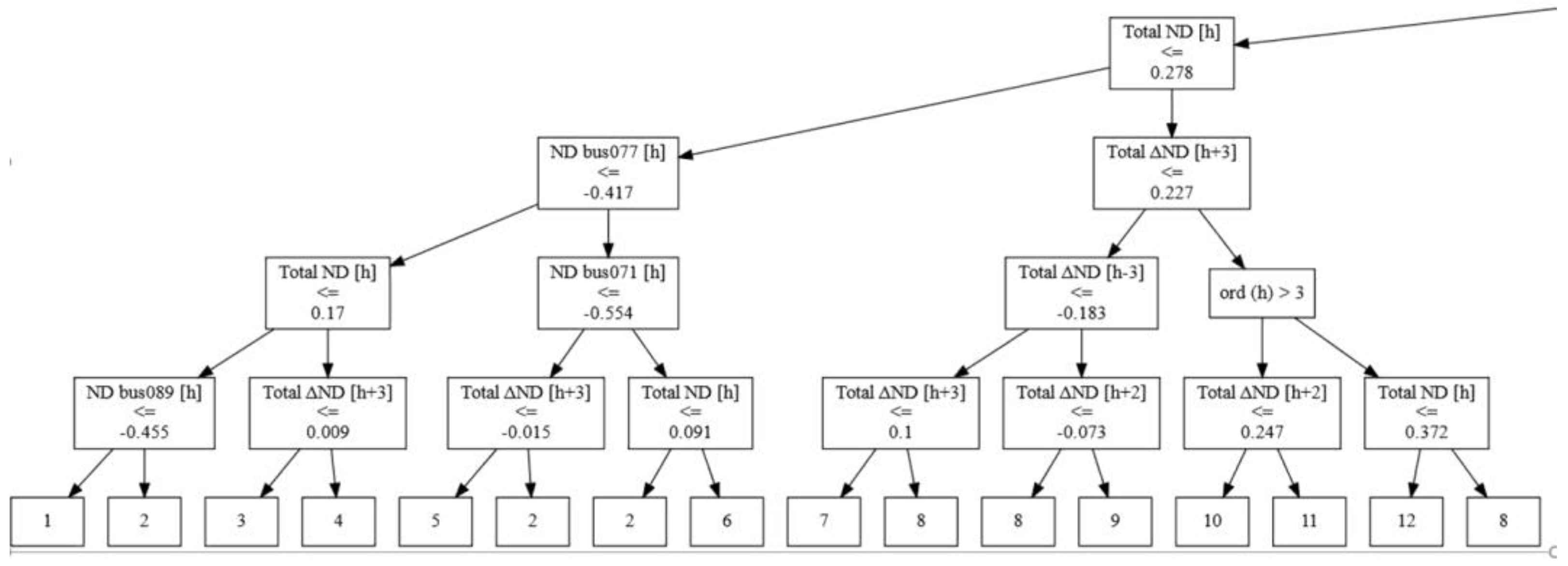
Figure 1. Commitment variable explained as a function of the scenario; fragment taken from [19].
Applsci 15 05732 g001
Figure 2. The three pillars of interpretable optimization.
Applsci 15 05732 g002
Figure 3. Simplification and surrogate modeling techniques.
Applsci 15 05732 g003
Figure 4. Plot of feasible region of optimization problem example. Redundant equations are represented with dashed lines.
Applsci 15 05732 g004
Figure 5. Near-optimal solution analysis techniques.
Applsci 15 05732 g005
Figure 6. Example of objective function value of near-optimal solutions, taken from [91]. The distribution of the objective function is much better than the general samples taken from the problem.
Applsci 15 05732 g006
Table 1. Summary of decomposition methods.
Benders’ DecompositionDantzig-WolfeLagrangian RelaxationADMM
Problem StructureComplicating variablesComplicating constraintsComplex constraintsSeparable objective
Best Suited forLP/MIP problems with complicating variables, continuous non-complicating onesLP problems with complicating constraintsProblems with nonlinear constraints Large-scale convex problems
Potential for InterpretabilityMediumLowMediumMedium
Table 2. Comparison of Morris method, Taguchi method, sequential analysis and optimal design.
Morris MethodTaguchi MethodSequential AnalysisOptimal Design
StrengthsSimple to implement and computationally efficient [68,69]Robust to noise factors and requires a reduced number of experiments [70]It is an adaptive method where experiments are based on previous results and it uses resources efficiently [66,71]It is a flexible and efficient method that can incorporate complicated constraints [67]
WeaknessesMostly qualitative and results may be unstable if there are strong nonlinearities [56,57]Less suited for complex iterations [72,73]It requires ongoing analyses and it is sensitive to initial sampling biases [74]It requires accurate model hypotheses [75]
Main aimIdentification of key variables at an early stageProblems where robustness is importantReduce number of experiments when problem features are unclearReduce number of experiments when problems are clear
Table 3. Summary of near-optimal solutions analysis methods.
MethodStrengthsWeaknesses
Sensitivity AnalysisIt is available in most solvers, and therefore its application is straightforward [96,97].It only evaluates the feasible region close to the optimal solution and offers limited performance if the problem is not linear [98].
Revised Simplex Method (with perturbation)It is computationally efficient [99].Its main usefulness relies on LP problems [100].
Modeling to Generate Alternatives (MGA)It maintains a balance between exploring the feasible region to generate near-optimal solutions and the computational burden [101].It may be computationally intense, and it does not guarantee a thorough exploration of each near-optimal zone of the feasible region [102,103].
K-optimal Solution AlgorithmsIt facilitates the decision-making process by providing solutions in a structured way [104].It may be difficult to apply to large-scale problems if the parameter k is very large because it requires executing the model k times [104].
Modeling All Alternatives (MAA)It performs an exhaustive evaluation of the feasible region and is guaranteed to find all near-optimal solutions closer than a specified threshold [86].It is very computationally intense [86].
Evolutionary Multi-Objective Optimization (EMO)It is particularly well suited for multiobjective problems and can deal with nonlinearities [105,106].It may need expert tuning of parameters, and there is no guarantee of optimality [107].
Fitness Landscape Analysis (FLA)It helps us understand features of complicated problems [108].It has seen minimal use in multiobjective problems so far [108].
Disclaimer/Publisher’s Note: The statements, opinions and data contained in all publications are solely those of the individual author(s) and contributor(s) and not of MDPI and/or the editor(s). MDPI and/or the editor(s) disclaim responsibility for any injury to people or property resulting from any ideas, methods, instructions or products referred to in the content.