Abstract
Grapes, highly nutritious and flavorful fruits, require adequate chlorophyll to ensure normal growth and development. Consequently, the rapid, accurate, and efficient detection of chlorophyll content is essential. This study develops a data-driven integrated framework that combines hyperspectral imaging (HSI) and convolutional neural networks (CNNs) to predict the chlorophyll content in grape leaves, employing hyperspectral images and chlorophyll a + b content data. Initially, the VGG16-U-Net model was employed to segment the hyperspectral images of grape leaves for leaf area extraction. Subsequently, the study discussed 15 different spectral preprocessing methods, selecting fast Fourier transform (FFT) as the optimal approach. Twelve one-dimensional CNN models were subsequently developed. Experimental results revealed that the VGG16-U-Net-FFT-CNN1-1 framework developed in this study exhibited outstanding performance, achieving an R2 of 0.925 and an RMSE of 2.172, surpassing those of traditional regression models. The t-test and F-test results further confirm the statistical robustness of the VGG16-U-Net-FFT-CNN1-1 framework. This provides a basis for estimating chlorophyll content in grape leaves using HSI technology.
1. Introduction
Grapes are highly nutritious and flavorful fruit with a long history of cultivation, remaining among the most widely produced fruits globally [1]. They offer numerous health benefits, including antioxidant and anti-inflammatory properties, modulation of gut microbiota, anti-obesity effects, and protective actions on the heart and liver as well as anti-diabetic and anti-cancer activities [2]. Beyond their consumption as fresh fruit, grapes have extensive applications in the food industry, contributing to products such as wine, grape juice, jams, raisins, and other derivatives [2,3]. Lorenz et al. categorized the phenology of the grapevine seasonal cycle into seven principal growth stages: budburst, leaf development, the appearance of inflorescences, flowering, fruit development, fruit maturation, and senescence [4]. Coombe proposed an alternative classification of the main grapevine growth stages, including budburst, shoots 10 cm, flowering begins, full bloom, setting, berries pea size, veraison, and harvest [5]. Regardless of the specific classification scheme, chlorophyll plays an indispensable role throughout the entire growth process of grapevines.
Chlorophyll is a group of green pigments found in higher plants and other photosynthetic organisms. Among the various types of chlorophyll, chlorophyll a and chlorophyll b are the main components, which are essential for the photosynthetic apparatus in terrestrial plants and green algae [6]. A deficiency in chlorophyll can result in leaf yellowing, poor growth and development, and reduced yield. As a fruit-bearing plant, grapevines require adequate chlorophyll to ensure normal growth and development. Changes in the chlorophyll content of grape leaves can also serve as a physiological index for responses and adaptation to UV-C radiation [7]. Therefore, the rapid, accurate, and efficient detection of chlorophyll content is crucial. Traditional methods for measuring chlorophyll content include spectrophotometry, fluorometry, high-performance liquid chromatography (HPLC), and portable chlorophyll meters [8,9,10,11]. However, these methods have limitations. While spectrophotometry, fluorometry, and HPLC provide accurate measurements, they require destructive sampling and the preservation of samples for laboratory analysis. Portable chlorophyll meters, such as SPAD-502 (Konica Minolta Inc., Tokyo, Japan), CL-01 (Hansatech Instruments Ltd., King’s Lynn, Norfolk, UK), Dualex Scientific+ (FORCE-A, Orsay, France), and CCM-200 (Opto-Sciences Inc., Tokyo, Japan), allow for non-destructive, low-cost, and low-labor measurements [12]. However, these devices often require multiple measurements to reduce variation, and their results are significantly affected by factors such as plant variety, cultivation practices, and environmental conditions. In recent years, hyperspectral imaging (HSI) technology has been extensively studied and proven to be an effective method for determining chlorophyll content in various plant species, including maize leaves [13], sugar beet [14], lettuce [15], wheat [16], and millet leaves [17].
HSI is capable of capturing multiple images at different wavelengths [18], simultaneously collecting both spatial and spectral data [19]. Compared to standard red, green, blue (RGB) images, HSI provides significantly more information. In agricultural production, hyperspectral remote sensing has been widely applied in crop growth monitoring, health assessment, resource allocation, yield estimation, and disease detection [19]. However, during the acquisition of spectral data, issues such as noise, baseline drift, and scattering can easily arise. Spectral preprocessing can reduce and eliminate the influence of various non-target factors [20], enhancing data quality and improving the accuracy and efficiency of subsequent analysis. Gao et al. applied Savitzky–Golay (SG) smoothing, adaptive window length SG smoothing, standard normal variate (SNV), and multiplicative scatter correction (MSC) algorithms to preprocess raw spectral data and constructed prediction models to analyze the effects of different preprocessing methods on model prediction accuracy [21]. Zhang et al. developed four preprocessing methods—SG, MSC, SNV, and variable sorting for normalization—to filter noise and scattering information from the raw spectra [22]. Yu et al. used MSC, SNV, and SG convolution smoothing for spectral preprocessing to facilitate subsequent analysis [23].
Convolutional neural networks (CNNs) are a type of feedforward neural network characterized by its ability to automatically learn features in tasks such as image and speech processing. CNNs possess a unique ability to extract spatial–spectral features, making them highly effective for processing hyperspectral images, and they are thus widely used in this field [24]. Pyo et al. proposed a point-centered regression CNN to estimate the concentrations of phycocyanin and chlorophyll a in water bodies using hyperspectral images, achieving coefficient of determination (R2) values greater than 0.86 and 0.73, respectively, with root mean square error (RMSE) values below 10 mg/m3 [25]. Luo et al. introduced an attention residual CNN, which, in combination with near-infrared HSI (900–1700 nm), predicted the fat content of salmon fillets, achieving an R2 of 0.9033, RMSE of prediction of 1.5143, and residual predictive deviation (RPD) of 3.2707 [26]. Li et al. employed short-wave infrared HSI combined with a one-dimensional (1D) CNN model to determine the soluble solids content in dried Hami jujube, and they achieved an R2 of 0.857, RMSE of 0.563, and RPD of 2.648 [27]. Ye et al. proposed a 1D deep learning model based on CNN with a spectral attention module to estimate the total chlorophyll content of greenhouse lettuce from full-spectrum hyperspectral images. The experimental results showed an average R2 of 0.746 and an average RMSE of 2.018, outperforming existing standard methods [15]. Wang et al. established an attention-CNN incorporating multi-feature parameter fusion to estimate chlorophyll content in millet leaves at different growth stages using hyperspectral images. The model achieved an R2 of 0.839, an RMSE of 1.451, and an RPD of 2.355, demonstrating superior predictive accuracy and regression fit compared to conventional models [17].
CNNs are currently among the most widely used models in deep learning [28]. In addition to the aforementioned regression tasks, they can also be applied to image segmentation. Image segmentation divides images into regions with different characteristics and extracts regions of interest (ROIs) [29], which can be understood as a pixel classification problem [28]. Compared to conventional RGB images, each spatial location in a hyperspectral image contains hundreds of spectral bands. Due to its high dimensionality [30], the image segmentation of hyperspectral images is more complex. Existing methods for hyperspectral image segmentation can be categorized into thresholding, watershed, clustering, morphological, region based segmentation, deep learning, and superpixel-based segmentation [31]. Among deep learning methods, commonly used CNN architectures include AlexNet [32], VGGNet [33], ResNet [34], GoogLeNet [35], MobileNet [36], and DenseNet [37]. CNN models have been widely applied to both classification and regression tasks.
The combination of HSI and CNN has yielded positive results in the field of agricultural production [19,24,38]. However, few studies have applied this combination to chlorophyll content regression models for grape leaves. Therefore, this study integrates hyperspectral image segmentation, spectral preprocessing, and CNNs to propose, for the first time, a data-driven ensemble framework for predicting chlorophyll a + b content in grape leaves. The specific objectives include (1) comparing the regression performance before and after hyperspectral image segmentation to demonstrate the effectiveness of ROI extraction through image segmentation; (2) discussing the optimal spectral preprocessing method for chlorophyll prediction models; and (3) selecting the most effective CNN model from the proposed self-developed CNN models, based on the extracted ROIs of grape leaves and the best preprocessing method, to predict the chlorophyll a + b content in grape leaves.
2. Materials and Methods
2.1. Experimental Dataset Construction
The dataset used in this study was published by Ryckewaert et al. from the University of Montpellier, France, in the journal Scientific Data, and it was made publicly available to support further research [39]. The experiment involved 204 grapevine leaves collected in September 2020 from southern France (GPS coordinates: 43.84208931745156, 1.8538190583140841) with an approximately equal proportion of red and white grape varieties [39]. Prior to sampling, the team measured the chlorophyll a + b content (µg/cm2) using the Dualex 311 Scientific+ TM (Force-A, Orsay, France).
Under controlled laboratory conditions, hyperspectral images of the 204 grapevine leaves were captured, covering a spectral range of 400–900 nm with a spectral resolution of 7 nm. The first and second dimensions of the acquired hyperspectral images correspond to the spatial positions (pixels), forming images of 512 × 512 pixels. The third dimension contains 204 spectral bands as spectral variables. Figure 1a–d show the RGB images, infrared band images, near-infrared band images, and normalized difference vegetation index (NDVI) images of the grape leaves, respectively.
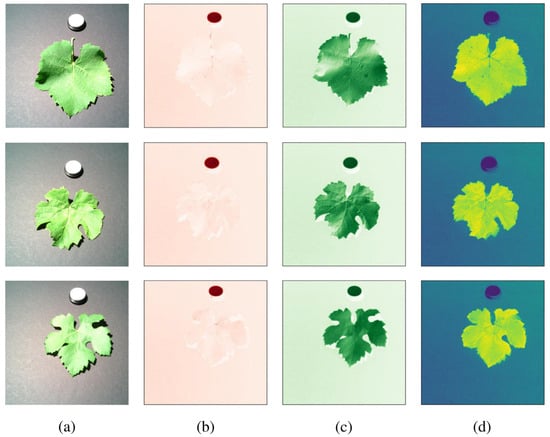
Figure 1.
(a) RGB images; (b) infrared band images; (c) near-infrared band images; (d) NDVI images.
Building upon the original HSI dataset, we constructed a novel annotated dataset through the pixel-accurate annotation of grape leaf boundaries in RGB images calculated from hyperspectral images, and we applied it to the hyperspectral image. Using the LabelMe annotation toolkit, we generated instance segmentation masks that maintain hyperspectral–spatial correspondence, and subsequent experiments were carried out on the constructed dataset. The constructed experimental dataset was divided into training and testing sets at a ratio of 8:2 for model development and evaluation.
2.2. Methods
This study developed an integrated framework that combined HSI and CNNs to predict the chlorophyll content in grape leaves, employing hyperspectral images and chlorophyll a + b content data. Figure 2 illustrates the workflow for chlorophyll content prediction in grape leaves. The process began with hyperspectral image segmentation using the VGG16-U-Net model, generating 204 ROI masked hyperspectral images. Following segmentation, spectral preprocessing was performed on the averaged reflectance spectra. Subsequently, 1D-CNN models were developed to predict the chlorophyll content of grape leaves with model performance evaluated through 10-fold cross-validation and compared against traditional regression models.
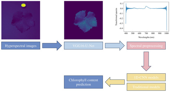
Figure 2.
Workflow for chlorophyll content prediction in grape leaves.
2.2.1. VGG16-U-Net
U-Net [40] implements jump connections, which connects and concatenates features from each layer of the encoder to the corresponding layers of the decoder, allowing for fine-grained image details [29]. VGG is commonly used as the backbone for the encoder in segmentation networks [29]. In this study, the encoder part of U-Net was replaced with the first 13 convolutional layers of VGG16 to build the VGG16-U-Net model, as shown in Figure 3. The VGG16-U-Net model was applied to segment the hyperspectral images of grape leaves, extracting the ROIs.
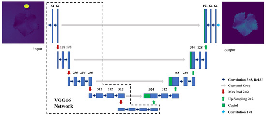
Figure 3.
Architecture of the VGG16-U-Net model.
The VGG16-U-Net model was used for binary classification between grape leaves and the background, retaining only the leaf regions. The confusion matrix for the binary classification is shown in Table 1.

Table 1.
Confusion matrix of the binary classification.
Subsequently, the results of the image segmentation were evaluated using three metrics: mean intersection over union (MIoU), mean pixel accuracy (MPA), and accuracy.
In the equations, represents the number of classes, and represents the total number of classes, including the background.
2.2.2. Spectral Preprocessing
Due to the high pixel resolution of the original hyperspectral images, this study calculated and analyzed the average spectra of 204 hyperspectral images of grape leaves.
The spectral preprocessing methods employed in this research include SNV, MSC, fast Fourier transform (FFT) [41], first derivative (FD), and second derivative (SD). These methods were combined in various ways to better capture spectral features.
SNV was applied to minimize spectral differences caused by variations in optical path, grain size distribution, and surface roughness among samples. Each sample was standardized by subtracting the mean and dividing by its own standard deviation [21]. SNV removes additive scattering without altering the original spectral shape, but it does not address multiplicative scattering [42]. MSC is commonly used to mitigate multiplicative scattering. The main objective of MSC is to reduce or eliminate the impact of physical properties such as particle size, shape, or surface roughness on spectral data [21]. FFT was employed for frequency domain analysis, transforming spectral data into the frequency domain. This facilitates the analysis and processing of periodic signals, noise filtering, and signal compression, helping to eliminate periodic noise components in the data. Derivatives have the capability to remove both additive and multiplicative effects from spectra. FD removes only the baseline, while SD removes both the baseline and linear trends [43]. To avoid excessively reducing the signal-to-noise ratio in the corrected spectra, SG smoothing was applied before FD and SD preprocessing [43].
2.2.3. Convolutional Neural Network
CNNs are inspired by the functionality of the human visual cortex and mimic human visual information processing [19]. As a prominent deep learning algorithm, CNNs have demonstrated exceptional performance in various spectral classification [44,45,46] and regression tasks [15,17,20,25,26,27]. A typical 1D-CNN consists of convolutional layers, pooling layers, a flattening layer, and fully connected layers. The convolutional layers extract features from spectral data by treating the spectra as 1D sequences. These features are then passed through fully connected layers to perform accurate prediction. The overall model flow of the 1D-CNN is illustrated in Figure 4. This study first constructed a specific 1D-CNN architecture for a regression task, with its layer-wise structure presented in Figure 5.
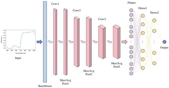
Figure 4.
Overall model flow of the 1D-CNN.
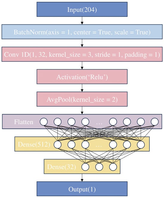
Figure 5.
Structure of the CNN model.
The network extracts spatial features from the input data through convolutional and pooling layers, comprising a series of convolution, activation, and pooling operations, which is followed by further processing and mapping through fully connected layers. Initially, a batch normalization layer is introduced, normalizing the input spectral reflectance to a mean of zero and a variance of one. This is followed by a 1D convolutional layer equipped with 32 filters, each with a kernel size of 3, and both stride and padding set to 1 to maintain the length of the data. The purpose of the convolutional layer is to extract local features from the input data. This is followed by a rectified linear unit (ReLU), which introduces non-linear processing to help the model learn complex feature representations. An average pooling layer then reduces the spatial dimensionality of the features, decreasing the complexity of subsequent computations and helping to reduce noise and the risk of overfitting. Subsequently, a flattening layer maps all feature maps into a 1D vector, preparing for processing by fully connected layers. Finally, three fully connected layers form the regression prediction part of the network. The first fully connected layer compresses the 3264-dimensional features from the convolutional layer down to 512 dimensions. The second fully connected layer further reduces the feature dimensions to 32. Each fully connected layer is followed by a ReLU activation function to maintain the model’s non-linearity. Ultimately, a fully connected layer with an output dimension of 1 generates the final prediction outcome—the chlorophyll a + b content predicted from the hyperspectral images of grape leaves. The constructed CNN model employs 10-fold cross-validation.
The CNN regression model is trained using an L2 loss function (MSE) and an adaptive moment estimation (Adam) optimizer. A predefined learning rate is used during the training phase. In the outset, the learning rate is set at 0.005, which is reduced by a factor of ten every 200 iterations. The learning rate is adjusted according to this schedule, and the training process is terminated once the loss stabilizes. The batch size is set to 32.
We designated the 1D-CNN regression model described earlier as CNN1-1 and subsequently developed several additional CNN models for further experimentation. The CNN architectures employed in this study are outlined in Table 2, Table 3 and Table 4.
Table 2.
CNN architectures with a single convolutional layer.
Table 3.
CNN architectures with two convolutional layers.
Table 4.
CNN architectures with three convolutional layers.
Table 2 presents four CNN models—CNN1-1, CNN1-2, CNN1-3, and CNN1-4—with a single convolutional layer. These models share a common architecture, differing only in the number of filters. Specifically, CNN1-1, CNN1-2, CNN1-3, and CNN1-4 contain 32, 64, 128, and 256 filters, respectively. Table 3 displays CNN models incorporating two convolutional layers: CNN2-1, CNN2-2, CNN2-3, and CNN2-4. In these models, the number of filters is consistent across layers. Specifically, CNN2-1 uses 32 filters per layer, CNN2-2 uses 64, CNN2-3 uses 128, and CNN2-4 uses 256 filters per layer. Table 4 illustrates CNN models with three convolutional layers: CNN3-1, CNN3-2, CNN3-3, and CNN3-4. Similar to the previous configurations, the number of filters in each layer remains consistent within each model. CNN3-1, CNN3-2, CNN3-3, and CNN3-4 use 32, 64, 128, and 256 filters per layer, respectively.
2.2.4. Traditional Regression Models
Support vector regression (SVR) is a widely used machine learning algorithm renowned for its excellent generalization capabilities, making it suitable for high-dimensional problem solving [20]. Random forest (RF) is a non-linear and non-parametric ensemble learning method that constructs multiple decision trees during training. When RF is used for the purpose of function approximation or regression, it is called random forest regression (RFR) [47]. Gradient boosting (GB) is an ensemble learner for both regression and classification [48]. Gradient boosting regression (GBR) builds a robust composite prediction model by combining multiple weak learners. Partial least squares regression (PLSR) is extensively used for the regression modeling of high-dimensional datasets [20].
In this study, the average spectra of 204 grape leaves and their corresponding chlorophyll a + b content were used to establish models using SVR, RFR, GBR, and PLSR.
2.2.5. Model Evaluation
The regression models for grape leaf chlorophyll content were evaluated using standard regression metrics, including the R2, mean square error (MSE), RMSE, and mean absolute error (MAE).
In the equations, represents the observed value of chlorophyll content, is the predicted value of chlorophyll content from the model, is the mean of the observed chlorophyll content values, and is the number of samples.
The closer the R2 value is to 1, the better the model fit. At the same time, the values for MSE, RMSE, and MAE should be as small as possible.
Additionally, to statistically assess prediction bias and reliability, a linear regression was fitted between the predicted and measured chlorophyll a + b values. The following statistical tests were conducted on the fitted line:
(1) A t-test was used to evaluate whether the slope significantly deviated from 1, indicating proportional agreement.
(2) A t-test was also performed on the intercept to test for significant bias.
(3) The standard error of prediction (SEP) was calculated to quantify the spread of prediction errors.
(4) Finally, an F-test was applied to compare the variance of SEP with the training error variance, serving as an overfitting diagnostic.
2.2.6. Experimental Environment
Table 5 describes the experimental environment used in this study.
Table 5.
Experimental environment.
3. Results
3.1. VGG16-U-Net Masked Images
In this study, the VGG16-U-Net model was employed to segment grape leaves in hyperspectral images by annotating, training, and testing on the RGB images calculated from the hyperspectral data. As a result, 204 mask images were generated from the calculated RGB images of grape leaves. These masks were then applied to the hyperspectral images, producing masked hyperspectral images of the grape leaves.
Using the sample “2020-09-10_013” as an example, Figure 6a displays the true RGB image captured by an RGB sensor. However, due to the positional offset between the RGB sensor and the hyperspectral camera, annotations cannot be directly made on the true RGB image. Therefore, the RGB image calculated from the hyperspectral image was used for annotation. Figure 6b shows the image before annotation, and Figure 6c shows the image after annotation. Figure 6d displays the hyperspectral image at a specific band, and by applying the mask generated through the aforementioned annotation and training process, we obtain the masked hyperspectral image at that specific band, as shown in Figure 6e.
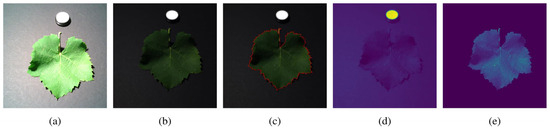
Figure 6.
(a) True RGB image; (b) RGB image calculated from the hyperspectral image; (c) example of data annotation; (d) hyperspectral image at a specific band; (e) masked hyperspectral image at a specific band.
After training with the VGG16-U-Net model, the mask images of the grape leaves in the test set achieved an MIoU of 98.34%, an MPA of 99.24%, and an accuracy of 99.64%, demonstrating the effectiveness of the segmentation for grape leaf images.
Table 6 shows the results of predicting the chlorophyll a + b content using the hyperspectral images before and after segmentation, utilizing the self-developed CNN1-1 model for training. As can be seen, compared to the original images, the results obtained using the segmented mask images were superior. The R2 improved from 0.867 to 0.904, and the RMSE decreased from 2.899 to 2.465. After 10-fold cross-validation, the R2 still improved from 0.822 to 0.847, and the RMSE decreased from 3.531 to 3.290. These results confirm the effectiveness of the image segmentation, and subsequent experiments will be conducted using the segmented mask images.
Table 6.
Results of the chlorophyll a + b content regression models using hyperspectral images before and after segmentation.
3.2. Impact of Different Preprocessing Methods on Regression Models
Before establishing regression models to predict the chlorophyll a + b content, this study applied 15 distinct preprocessing methods to the average spectra of the segmented grape leaf hyperspectral images. These methods include SNV, MSC, FFT, FD, SD, and combinations thereof such as SNV + FFT, SNV + FD, SNV + SD, MSC + FFT, MSC + FD, MSC + SD, FFT + FD, FFT + SD, FD + FFT, and SD + FFT. The objective was to explore the impact of spectral preprocessing on the performance of regression models. Figure 7 presents the comparative spectral profiles of grape leaves, showing both the original mean reflectance spectra and their transformed counterparts after spectral preprocessing.
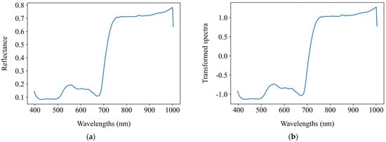
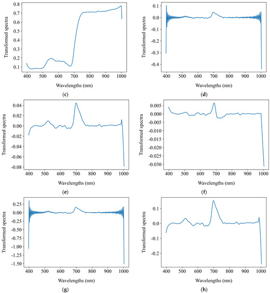
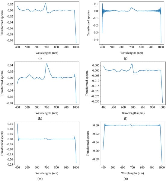
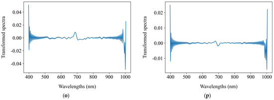
Figure 7.
The original mean reflectance spectra and the mean transformed counterparts after spectral preprocessing. (a) Original spectra; (b) SNV; (c) MSC; (d) FFT; (e) FD; (f) SD; (g) SNV + FFT; (h) SNV + FD; (i) SNV + SD; (j) MSC + FFT; (k) MSC + FD; (l) MSC + SD; (m) FFT + FD; (n) FFT + SD; (o) FD + FFT; (p) SD + FFT.
Chlorophyll a + b content predictions were performed using the self-developed CNN1-1 model with the results displayed in Table 7. Among the 15 preprocessing methods, the top five performing were FFT, SNV + FD, MSC + FD, SNV + FFT, and MSC + FFT. Following spectral preprocessing, there was a noticeable improvement in R2 and a reduction in RMSE both before and after 10-fold cross-validation. The FFT preprocessing method improved R2 from 0.904 to 0.925 and reduced RMSE from 2.465 to 2.172 with 10-fold cross-validation further improving R2 to 0.880 and reducing RMSE to 2.983. The SNV + FD combination achieved an R2 of 0.917 and an RMSE of 2.291 with cross-validation results of R2 at 0.870 and RMSE at 3.069. The MSC + FD combination resulted in an R2 of 0.917 and an RMSE of 2.294 with cross-validation results of R2 at 0.869 and RMSE at 3.089. The SNV + FFT combination reached an R2 of 0.916 and an RMSE of 2.300 with a post cross-validation R2 of 0.869 and RMSE of 3.070. Lastly, the MSC + FFT combination showed an R2 of 0.913 and an RMSE of 2.341 with cross-validation results of R2 at 0.866 and RMSE at 3.059.
Table 7.
Results of the chlorophyll a + b content regression models using different preprocessing methods.
Among these methods, FFT preprocessing yielded the best outcomes, attaining the highest pre- and post-cross-validation R2 values of 0.925 and 0.880, respectively. The efficacy of the FFT spectral preprocessing method was validated, making it the chosen uniform preprocessing method for regression model comparisons in the subsequent sections.
3.3. Evaluation of CNN Models for Accurate Prediction of Chlorophyll a + b Content
To establish regression models for predicting the chlorophyll a + b content of 204 grape leaf hyperspectral images, the dataset was divided into a training set and a test set in an 8:2 ratio. Using the average spectra of the grape leaves obtained after image segmentation and FFT spectral preprocessing, traditional regression models—including SVR, RFR, GBR, and PLSR—as well as 12 CNN models were built to predict the chlorophyll a + b content of grape leaves. The regression models were evaluated using various performance metrics.
Table 8 displays the results of the 12 self-developed CNN models compared to the four traditional regression models. The CNN1-1 model achieved an R2 of 0.925 and an RMSE of 2.172 with 10-fold cross-validation results showing an R2 of 0.880 and an RMSE of 2.983. The R2 of the CNN1-2 model was 0.923 with an RMSE of 2.204, and after 10-fold cross-validation, the R2 was 0.874 and the RMSE was 3.003. The CNN1-3 model had an R2 of 0.921 and an RMSE of 2.230 with 10-fold cross-validation results showing an R2 of 0.872 and an RMSE of 3.025. The CNN1-4 model achieved an R2 of 0.925 and an RMSE of 2.173 with 10-fold cross-validation results showing an R2 of 0.879 and an RMSE of 2.944. The CNN2-1 model recorded an R2 of 0.919 and an RMSE of 2.266 with 10-fold cross-validation results showing an R2 of 0.861 and an RMSE of 3.109. The CNN2-2 model had an R2 of 0.915 and an RMSE of 2.312 with 10-fold cross-validation results showing an R2 of 0.858 and an RMSE of 3.156. The CNN2-3 model exhibited an R2 of 0.920 and an RMSE of 2.250 with 10-fold cross-validation results showing an R2 of 0.862 and an RMSE of 3.128. The CNN2-4 model recorded an R2 of 0.919 and an RMSE of 2.259 with 10-fold cross-validation results showing an R2 of 0.860 and an RMSE of 3.138. The CNN3-1 model had an R2 of 0.917 and an RMSE of 2.288 with 10-fold cross-validation results showing an R2 of 0.859 and an RMSE of 3.135. The CNN3-2 model showed an R2 of 0.917 and an RMSE of 2.288 with 10-fold cross-validation results showing an R2 of 0.859 and an RMSE of 3.126. The CNN3-3 model recorded an R2 of 0.916 and an RMSE of 2.303 with 10-fold cross-validation results showing an R2 of 0.859 and an RMSE of 3.151. The CNN3-4 model achieved an R2 of 0.829 and an RMSE of 3.286 with 10-fold cross-validation results showing an R2 of 0.806 and an RMSE of 3.388.
Table 8.
Results of different chlorophyll a + b content regression models.
The SVR model had an R2 of 0.131 and an RMSE of 7.407 with 10-fold cross-validation results of R2 at 0.148 and RMSE at 8.302. The RFR model recorded an R2 of 0.879 and an RMSE of 2.760 with 10-fold cross-validation R2 of 0.794 and RMSE of 3.781. The GBR model showed an R2 of 0.871 and an RMSE of 2.853 with 10-fold cross-validation results of R2 at 0.813 and RMSE at 3.663. The PLSR model demonstrated an R2 of 0.771 and an RMSE of 3.805 with 10-fold cross-validation results of R2 at 0.769 and RMSE of 4.100.
Experimental results indicate that compared to traditional regression models, the CNN models developed in this study generally outperformed the conventional methods. Among all the models evaluated, the self-developed CNN1-1 model showed optimal performance, achieving the highest R2 of 0.925 and maintaining an R2 of 0.880 even after 10-fold cross-validation. It also exhibited the lowest MSE and RMSE, thereby providing a more accurate prediction of the chlorophyll a + b content in grape leaves. This superior performance can be attributed to the strong feature learning capability of CNNs, which enables them to effectively capture the complex mapping between spectral information and chlorophyll content.
Traditional machine learning models such as SVR, RFR, GBR, and PLSR offer relatively high interpretability and reasonable modeling capabilities in hyperspectral analysis. They are particularly robust when working with limited sample sizes or under high-noise conditions. However, these models typically rely on manual feature selection or dimensionality reduction, which limits their ability to fully exploit the intricate non-linear structures and local spectral correlations between bands contained in high-dimensional spectral data.
In contrast, CNNs, as a deep learning approach, possess powerful automatic feature extraction capabilities. Through their multi-layer convolutional architecture, CNNs can learn hierarchical feature representations directly from raw spectra, effectively capturing complex non-linear relationships between spectral features and target variables without human intervention. Moreover, CNNs are particularly effective at identifying local spectral continuity and inter-band dependencies. As a result, they generally achieve better prediction performance and stronger generalization ability compared to traditional methods.
3.4. Statistical Validation of Prediction Performance
To further validate the predictive accuracy and generalization capability of the best-performing CNN1-1 model, a series of statistical validation analyses were conducted.
A scatter plot of the predicted versus measured chlorophyll a + b content was generated, and a linear regression line was fitted to visualize their relationship, as shown in Figure 8.
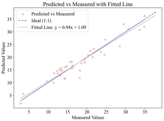
Figure 8.
Relationship between predicted and measured chlorophyll a + b content.
The R2 was 0.925, indicating a strong correlation and high predictive accuracy. The regression equation was
To assess the statistical reliability of the predictions, two one-sample t-tests were performed. First, the slope was tested against the ideal value of 1. The result (t = −1.427, p = 0.161) showed no significant deviation, indicating that the predicted values are proportional to the measured chlorophyll content. Second, the intercept (bias) was tested against 0, yielding t = −0.152, p = 0.880, which suggests no significant systematic bias between the predicted and actual values.
The SEP was calculated to be 2.199 µg/cm2, reflecting the typical deviation of predicted values from the reference measurements. To evaluate potential overfitting, an F-test was conducted to compare the variance of SEP with that of the training error. The result (F = 0.454, p = 0.993) showed no significant difference, providing statistical evidence that the model generalizes well and is not overfitted to the training data.
Collectively, these validation results demonstrate that the CNN1-1 model delivers robust predictive performance with high accuracy, minimal bias, and strong generalization ability.
4. Discussion
This study demonstrates the feasibility and effectiveness of integrating HSI with CNNs for predicting chlorophyll a + b content in grapevine leaves. By employing the VGG16-U-Net model for hyperspectral image segmentation, the approach enables the automatic extraction of leaf regions and reduces background noise interference—offering a distinct advantage over many traditional spectral studies that rely on manual region selection.
For spectral preprocessing, spectral preprocessing methods such as FFT, SNV + FD, MSC + FD, SNV + FFT, and MSC + FFT significantly enhanced the prediction accuracy of chlorophyll a + b content. However, some methods, such as SNV, MSC, SD, and SNV + SD, actually reduced model performance. The proper choice of preprocessing is difficult to assess prior to model validation [43]. Although previous studies have predominantly employed common preprocessing methods such as SNV or FD, our findings reveal that FFT preprocessing—despite being less commonly used—produced the most effective results. This suggests that frequency-domain transformations can effectively capture periodic or structural patterns in the spectral data that are associated with chlorophyll concentration. Such information may not be readily apparent in the original or derivative spectra, highlighting the potential of FFT as a valuable preprocessing technique for spectral regression tasks.
Interestingly, the shallow CNN architecture (CNN1-1) outperformed deeper and more complex models, indicating that increased network depth or complexity does not necessarily lead to improved performance—especially when feature extraction is already supported by appropriate preprocessing and ROI segmentation. This finding may be attributed to the relatively small sample size in this study, where deeper networks are more prone to overfitting.
To further evaluate the performance of the proposed VGG16-U-Net-FFT-CNN1-1 framework for chlorophyll content prediction, we compared its results with those reported in previous studies that also utilized hyperspectral imaging for chlorophyll estimation. As shown in Table 9, the proposed VGG16-U-Net-FFT-CNN1-1 framework outperformed the models developed by Ye et al. [15], Yang et al. [16], and Wang et al. [17], offering a novel and more effective approach to chlorophyll content prediction.
Table 9.
Comparison between the proposed VGG16-U-Net-FFT-CNN1-1 model and other chlorophyll prediction models.
From a practical perspective, this approach offers a non-destructive, efficient, and scalable solution for monitoring plant physiological traits. Within the context of precision agriculture, these models could be embedded into field-deployable platforms to support rapid chlorophyll diagnostics, facilitate nutrient management, and enable early stress detection. However, this study was based on hyperspectral data collected at a single time point. Future work will focus on expanding the dataset to encompass the entire growth cycle of grapevines, enabling the model to be generalized across different developmental stages. Additionally, this research will not be limited to chlorophyll content but will also focus on other plant physiological and biochemical indicators—such as nitrogen content, leaf water status, and disease markers—in order to establish a more comprehensive and integrated crop monitoring framework. In addition, future research will consider other crops of higher economic value and scientific significance.
5. Conclusions
This study proposed a data-driven integrated framework that combines HSI technology and CNNs for the rapid, accurate, and efficient prediction of chlorophyll a + b content in grape leaves, using hyperspectral images and corresponding chlorophyll a + b content data as inputs.
Initially, the self-developed CNN1-1 model constructed from the original average spectra achieved an R2 of 0.867 and an RMSE of 2.899. The VGG16-U-Net model was then used to segment the hyperspectral images, resulting in an improved R2 of 0.904 and a reduced RMSE of 2.465. Subsequently, the best spectral preprocessing method, FFT, was selected from 15 options to construct CNN1-1 model on the average spectra of ROIs, leading to further enhancement in R2. Compared to a series of traditional regression models such as SVR, RFR, GBR, and PLSR, CNN1-1 among the self-developed CNN models demonstrated superior performance. The proposed VGG16-U-Net-FFT-CNN1-1 framework achieved an R2 of 0.925 and an RMSE of 2.172, indicating its strong potential for accurate chlorophyll content estimation in grape leaves. After 10-fold cross-validation, the R2 and RMSE were 0.880 and 2.983, respectively, indicating that the chlorophyll a + b regression model combining HSI technology with CNN produced commendable results. The t-test and F-test results further confirm the statistical robustness of the VGG16-U-Net-FFT-CNN1-1 framework. Future research will consider increasing the sample size and spectral variability to further enhance the model’s robustness.
Author Contributions
Conceptualization, L.S. and J.X.; methodology, M.Z.; software, M.Z.; validation, L.W. and J.X.; formal analysis, X.Z.; investigation, X.Z.; resources, X.Z.; data curation, M.Z. and J.X.; writing—original draft preparation, M.Z.; writing—review and editing, M.Z.; visualization, L.W.; supervision, L.S.; project administration, L.S.; funding acquisition, L.S. All authors have read and agreed to the published version of the manuscript.
Funding
This research received no external funding.
Institutional Review Board Statement
Not applicable.
Informed Consent Statement
Not applicable.
Data Availability Statement
The original contributions presented in this study are included in the article. Further inquiries can be directed to the corresponding author(s).
Conflicts of Interest
The authors declare no conflicts of interest.
Abbreviations
The following abbreviations are used in this manuscript:
| 1D | one-dimensional |
| CNN | convolutional neural network |
| FD | first derivative |
| FFT | fast Fourier transform |
| GB | gradient boosting |
| GBR | gradient boosting regression |
| HPLC | high-performance liquid chromatography |
| HSI | hyperspectral imaging |
| MAE | mean absolute error |
| MIoU | mean intersection over union |
| MPA | mean pixel accuracy |
| MSC | multiplicative scatter correction |
| MSE | mean square error |
| NDVI | normalized difference vegetation index |
| PLSR | partial least squares regression |
| R2 | coefficient of determination |
| ReLU | rectified linear unit |
| RF | random forest |
| RFR | random forest regression |
| RGB | red, green, blue |
| RMSE | root mean square error |
| ROI | region of interest |
| RPD | residual predictive deviation |
| SD | second derivative |
| SEP | standard error of prediction |
| SG | Savitzky–Golay |
| SNV | standard normal variate |
| SVR | support vector regression |
References
- Restani, P.; Fradera, U.; Ruf, J.C.; Stockley, C.; Teissedre, P.L.; Biella, S.; Colombo, F.; Lorenzo, C.D. Grapes and their derivatives in modulation of cognitive decline: A critical review of epidemiological and randomized-controlled trials in humans. Crit. Rev. Food Sci. Nutr. 2021, 61, 566–576. [Google Scholar] [CrossRef] [PubMed]
- Zhou, D.D.; Li, J.; Xiong, R.G.; Saimaiti, A.; Huang, S.Y.; Wu, S.X.; Yang, Z.J.; Shang, A.; Zhao, C.N.; Gan, R.Y.; et al. Bioactive Compounds, Health Benefits and Food Applications of Grape. Foods 2022, 11, 2755. [Google Scholar] [CrossRef] [PubMed]
- Kandylis, P.; Dimitrellou, D.; Moschakis, T. Recent applications of grapes and their derivatives in dairy products. Trends Food Sci. Technol. 2021, 114, 696–711. [Google Scholar] [CrossRef]
- Lorenz, D.H.; Eichhorn, K.W.; Bleiholder, H.; Klose, R.; Meier, U.; Weber, E. Growth Stages of the Grapevine: Phenological Growth Stages of the Grapevine (Vitis vinifera L. ssp. Vinifera)—Codes and Descriptions According to the Extended BBCH Scale. Aust. J. Grape Wine Res. 1995, 1, 100–103. [Google Scholar] [CrossRef]
- Coombe, B.G. Growth Stages of the Grapevine: Adoption of a system for identifying grapevine growth stages. Aust. J. Grape Wine Res. 1995, 1, 104–110. [Google Scholar] [CrossRef]
- Tanaka, R.; Tanaka, A. Chlorophyll cycle regulates the construction and destruction of the light-harvesting complexes. Biochim. Et Biophys. Acta (BBA)-Bioenerg. 2011, 1807, 968–976. [Google Scholar] [CrossRef]
- Luo, Y.Y.; Li, R.X.; Jiang, Q.S.; Bai, R.; Duan, D. Changes in the chlorophyll content of grape leaves could provide a physiological index for responses and adaptation to UV-C radiation. Nord. J. Bot. 2019, 37, 1–11. [Google Scholar] [CrossRef]
- Croft, H.; Chen, J.M. Leaf pigment content. Compr. Remote Sens. 2018, 3, 117–142. [Google Scholar]
- Ritchie, R.J. Consistent sets of spectrophotometric chlorophyll equations for acetone, methanol and ethanol solvents. Photosynth. Res. 2006, 89, 27–41. [Google Scholar] [CrossRef]
- Dugo, P.; Cacciola, F.; Kumm, T.; Dugo, G.; Mondello, L. Comprehensive multidimensional liquid chromatography: Theory and applications. J. Chromatogr. A 2008, 1184, 353–368. [Google Scholar] [CrossRef]
- Dong, T.; Shang, J.; Chen, J.M.; Liu, J.; Qian, B.; Ma, B.; Morrison, M.J.; Zhang, C.; Liu, Y.; Shi, Y.; et al. Assessment of Portable Chlorophyll Meters for Measuring Crop Leaf Chlorophyll Concentration. Remote Sens. 2019, 11, 2706. [Google Scholar] [CrossRef]
- Jacquemoud, S.; Ustin, S. Leaf Optical Properties; Cambridge University Press: Cambridge, UK, 2019. [Google Scholar]
- Gao, D.; Li, M.; Zhang, J.; Song, D.; Sun, H.; Qiao, L.; Zhao, R. Improvement of chlorophyll content estimation on maize leaf by vein removal in hyperspectral image. Comput. Electron. Agric. 2021, 184, 106077. [Google Scholar] [CrossRef]
- Zhang, J.; Tian, H.; Wang, D.; Li, H.; Mouazen, A.M. A novel spectral index for estimation of relative chlorophyll content of sugar beet. Comput. Electron. Agric. 2021, 108, 106088. [Google Scholar] [CrossRef]
- Ye, Z.; Tan, X.; Dai, M.; Chen, X.; Zhong, Y.; Zhang, Y.; Ruan, Y.; Kong, D. A hyperspectral deep learning attention model for predicting lettuce chlorophyll content. Plant Methods 2024, 20, 22. [Google Scholar] [CrossRef]
- Yang, Y.; Nan, R.; Mi, T.; Song, Y.; Shi, F.; Liu, X.; Wang, Y.; Sun, F.; Xi, Y.; Zhang, C. Rapid and Nondestructive Evaluation of Wheat Chlorophyll under Drought Stress Using Hyperspectral Imaging. Int. J. Mol. Sci. 2023, 24, 5825. [Google Scholar] [CrossRef]
- Wang, X.; Li, Z.; Wang, W.; Wang, J. Chlorophyll content for millet leaf using hyperspectral imaging and an attention-convolutional neural network. Ciênc. Rural 2020, 50, e20190731. [Google Scholar] [CrossRef]
- Chang, C.I. Hyperspectral Imaging: Techniques for Spectral Detection and Classification; Springer Science & Business Media: Berlin/Heidelberg, Germany, 2003. [Google Scholar]
- Guerri, M.F.; Distante, C.; Spagnolo, P.; Bougourzi, F.; Taleb-Ahmed, A. Deep learning techniques for hyperspectral image analysis in agriculture: A review. ISPRS Open J. Photogramm. Remote Sens. 2024, 12, 100062. [Google Scholar] [CrossRef]
- Xiao, Q.; Tang, W.; Zhang, C.; Zhou, L.; Feng, L.; Shen, J.; Yan, T.; Gao, P.; He, Y.; Wu, N. Spectral preprocessing combined with deep transfer learning to evaluate chlorophyll content in cotton leaves. Plant Phenomics 2022, 2022, 9813841. [Google Scholar] [CrossRef]
- Gao, W.; Cheng, X.; Liu, X.; Han, Y.; Ren, Z. Apple firmness detection method based on hyperspectral technology. Food Control 2024, 166, 110690. [Google Scholar] [CrossRef]
- Zhang, X.; Sun, J.; Li, P.; Zeng, F.; Wang, H. Hyperspectral detection of salted sea cucumber adulteration using different spectral preprocessing techniques and SVM method. LWT 2021, 152, 112295. [Google Scholar] [CrossRef]
- Yu, H.; Hu, Y.; Qi, L.; Zhang, K.; Jiang, J.; Li, H.; Zhang, X.; Zhang, Z. Hyperspectral Detection of Moisture Content in Rice Straw Nutrient Bowl Trays Based on PSO-SVR. Sustainability 2023, 15, 8703. [Google Scholar] [CrossRef]
- Shuai, L.; Li, Z.; Chen, Z.; Luo, D.; Mu, J. A research review on deep learning combined with hyperspectral Imaging in multiscale agricultural sensing. Comput. Electron. Agric. 2024, 217, 108577. [Google Scholar] [CrossRef]
- Pyo, J.C.; Duan, H.; Baek, S.; Kim, M.S.; Jeon, T.; Kwon, Y.S.; Lee, H.; Cho, K.H. A convolutional neural network regression for quantifying cyanobacteria using hyperspectral imagery. Remote Sens. Environ. 2019, 233, 111350. [Google Scholar] [CrossRef]
- Luo, W.; Zhang, J.; Huang, H.; Peng, W.; Gao, Y.; Zhan, B.; Zhang, H. Prediction of fat content in salmon fillets based on hyperspectral imaging and residual attention convolution neural network. LWT 2023, 184, 115018. [Google Scholar] [CrossRef]
- Li, Y.; Ma, B.; Li, C.; Yu, G. Accurate prediction of soluble solid content in dried Hami jujube using SWIR hyperspectral imaging with comparative analysis of models. Comput. Electron. Agric. 2022, 193, 106655. [Google Scholar] [CrossRef]
- Minaee, S.; Boykov, Y.; Porikli, F.; Plaza, A.; Kehtarnavaz, N.; Terzopoulos, D. Image segmentation using deep learning: A survey. IEEE Trans. Pattern Anal. Mach. Intell. 2021, 44, 3523–3542. [Google Scholar] [CrossRef]
- Yu, Y.; Wang, C.; Fu, Q.; Kou, R.; Huang, F.; Yang, B.; Yang, T.; Gao, M. Techniques and Challenges of Image Segmentation: A Review. Electronics 2023, 12, 1199. [Google Scholar] [CrossRef]
- Deng, Y.J.; Yang, M.L.; Li, H.C.; Long, C.F.; Fang, K.; Du, Q. Feature Dimensionality Reduction with L2, p-Norm-Based Robust Embedding Regression for Classification of Hyperspectral Images. IEEE Trans. Geosci. Remote Sens. 2024, 62, 1–14. [Google Scholar] [CrossRef]
- Grewal, R.; Kasana, S.S.; Kasana, G. Hyperspectral image segmentation: A comprehensive survey. Multimed. Tools Appl. 2023, 82, 20819–20872. [Google Scholar] [CrossRef]
- Krizhevsky, A.; Sutskever, I.; Hinton, G.E. Imagenet Classification with Deep Convolutional Neural Networks. Commun. ACM 2017, 60, 84–90. [Google Scholar] [CrossRef]
- Simonyan, K.; Zisserman, A. Very Deep Convolutional Networks for Large-Scale Image Recognition. In Proceedings of the International Conference on Learning Representations, San Diego, CA, USA, 7–9 May 2015. [Google Scholar]
- He, K.; Zhang, X.; Ren, S.; Sun, J. Deep residual learning for image recognition. In Proceedings of the Conference on Computer Vision and Pattern Recognition, Las Vegas, NV, USA, 27–30 June 2016. [Google Scholar]
- Szegedy, C.; Liu, W.; Jia, Y.; Sermanet, P.; Reed, S.; Anguelov, D.; Rabinovich, A. Going deeper with convolutions. In Proceedings of the Conference on Computer Vision and Pattern Recognition, Boston, MA, USA, 7–12 June 2015. [Google Scholar]
- Howard, A.G.; Zhu, M.; Chen, B.; Kalenichenko, D.; Wang, W.; Weyand, T.; Andreetto, M.; Adam, H. Mobilenets: Efficient convolutional neural networks for mobile vision applications. arXiv 2017, arXiv:1704.04861. [Google Scholar]
- Huang, G.; Liu, Z.; Van Der Maaten, L.; Weinberger, K.Q. Densely connected convolutional networks. In Proceedings of the IEEE Conference on Computer Vision and Pattern Recognition (CVPR), Honolulu, HI, USA, 21–26 July 2017; pp. 4700–4708. [Google Scholar]
- Barbedo, J.G.A. A review on the combination of deep learning techniques with proximal hyperspectral images in agriculture. Comput. Electron. Agric. 2023, 210, 107920. [Google Scholar] [CrossRef]
- Ryckewaert, M.; Héran, D.; Trani, J.P.; Mas-Garcia, S.; Feilhes, C.; Prezman, F.; Serrano, E.; Bendoula, R. Hyperspectral images of grapevine leaves including healthy leaves and leaves with biotic and abiotic symptoms. Sci. Data 2023, 10, 743. [Google Scholar] [CrossRef]
- Ronneberger, O.; Fischer, P.; Brox, T. U-Net: Convolutional Networks for Biomedical Image Segmentation. In Medical Image Computing and Computer-Assisted Intervention—MICCAI 2015, Proceedings of the 18th International Conference, Munich, Germany, 5–9 October 2015; Navab, N., Hornegger, J., Wells, W.M., Frangi, A.F., Eds.; Springer: Berlin/Heidelberg, Germany, 2015; Volume 9351, pp. 234–241. [Google Scholar] [CrossRef]
- Zhu, S.; Chao, M.; Zhang, J.; Xu, X.; Song, P.; Zhang, J.; Huang, Z. Identification of Soybean Seed Varieties Based on Hyperspectral Imaging Technology. Sensors 2019, 19, 5225. [Google Scholar] [CrossRef]
- Cozzolino, D.; Williams, P.J.; Hoffman, L.C. An overview of pre-processing methods available for hyperspectral imaging applications. Microchem. J. 2023, 193, 109129. [Google Scholar] [CrossRef]
- Rinnan, Å.; van den Berg, F.; Engelsen, S.B. Review of the most common pre-processing techniques for near-infrared spectra. TrAC Trends Anal. Chem. 2009, 28, 1201–1222. [Google Scholar] [CrossRef]
- Feng, L.; Wu, B.; He, Y.; Zhang, C. Hyperspectral imaging combined with deep transfer learning for rice disease detection. Front. Plant Sci. 2021, 12, 693521. [Google Scholar] [CrossRef]
- Zhang, J.; Yang, Y.; Feng, X.; Xu, H.; Chen, J.; He, Y. Identification of bacterial blight resistant rice seeds using terahertz imaging and hyperspectral imaging combined with convolutional neural network. Front. Plant Sci. 2020, 11, 821. [Google Scholar] [CrossRef]
- Yan, T.; Xu, W.; Lin, J.; Duan, L.; Gao, P.; Zhang, C.; Lv, X. Combining multi-dimensional convolutional neural network (CNN) with visualization method for detection of aphis gossypii glover infection in cotton leaves using hyperspectral imaging. Front. Plant Sci. 2021, 12, 604510. [Google Scholar] [CrossRef]
- Desai, S.; Ouarda, T.B.M.J. Regional hydrological frequency analysis at ungauged sites with random forest regression. J. Hydrol. 2021, 594, 125861. [Google Scholar] [CrossRef]
- Cai, J.; Xu, K.; Zhu, Y.; Hu, F.; Li, L. Prediction and analysis of net ecosystem carbon exchange based on gradient boosting regression and random forest. Appl. Energy 2020, 262, 114566. [Google Scholar] [CrossRef]
Disclaimer/Publisher’s Note: The statements, opinions and data contained in all publications are solely those of the individual author(s) and contributor(s) and not of MDPI and/or the editor(s). MDPI and/or the editor(s) disclaim responsibility for any injury to people or property resulting from any ideas, methods, instructions or products referred to in the content. |
© 2025 by the authors. Licensee MDPI, Basel, Switzerland. This article is an open access article distributed under the terms and conditions of the Creative Commons Attribution (CC BY) license (https://creativecommons.org/licenses/by/4.0/).