The Impact of Gravity on Different Height Systems: A Case Study on Mt. Medvednica

Abstract

This study examines the influence of gravity on different height systems by integrating Global Navigation Satellite Systems (GNSS), leveling, and gravimetric measurements. Although the theoretical influence of gravity on height systems is well known, empirical studies that quantify these effects along steep terrain are rare—particularly within the Croatian reference systems. Geometric leveling, recognized for its precision in geodesy, was employed alongside gravimetric data to analyze the relationship between gravity variations and height differences. The research was conducted along Sljeme Road on Mt. Medvednica, Croatia, where altitude-dependent gravity effects were systematically investigated along an elevation profile with a height difference of about 650 m. GNSS measurements provided positional coordinates referenced to the Croatian Terrestrial Reference System 1996 (HTRS96) (EPSG:4888), while leveling and gravimetric data were analyzed within the Croatian Height Reference System 1971 (HVRS71) (EPSG:5610) and Croatian Gravimetric Reference System 2003 (HGRS03), respectively. The results demonstrate that differences between geometric and normal–orthometric heights become more pronounced at higher elevations but remain at the millimeter level. Notably, the impact of gravity is evident in normal and orthometric heights, with differences from geometric heights reaching up to 3.7 cm at the highest points. Additionally, a comparison between normal and orthometric heights reveals that at the beginning of the leveling line, the difference is around 4 mm. However, as the elevation increases, this difference grows, reaching over 1 cm at the end of the leveling line. The study also confirms the theoretical correlation between the geoid–quasigeoid height difference and terrain elevation, with increasing differences observed at higher altitudes. To examine the consistency of different height determination methods, two approaches were applied: one based on adjustment within the geopotential system, and the other involving direct adjustment in the desired height system, with specific height corrections applied. The results confirmed that the height differences between the two methods were 0, to the tenth of a millimeter, indicating that both methods provided identical results. These findings contribute to a deeper understanding of geodetic height systems and the role of gravity in height determination.

1. Introduction

To investigate the influence of gravity on different height systems, this study combined GNSS, leveling, and gravimetric measurements. Global Navigation Satellite Systems (GNSS) represent a collective term for all the satellite systems used for navigation and positioning. GNSS measurements provided positional coordinates for points that served as reference markers for gravimetric measurements and geometric leveling. Considering the level of accuracy required to validate the hypothesis, precise geometric leveling was employed, which is recognized as the most accurate method for determining height differences in geodesy. Geometric leveling operates within the real field of gravity, where even under ideal conditions, the sum of height differences in a closed leveling loop would not be exactly zero due to the influence of the leveling path.

The main objective of this study is to analyze how gravity affects different types of heights derived from leveling, such as orthometric, normal, and normal–orthometric heights. The methodology involves comparing these height types by integrating precise geometric leveling data with gravity measurements along a steep terrain profile. GNSS was used exclusively to establish horizontal positions and support the stabilization of benchmarks, while gravity data enabled the determination of corresponding height systems.

To address this, gravimetric measurements were incorporated alongside leveling measurements, allowing the integration of gravity data with height differences. The study area was chosen to maximize the observable effects of gravity, which generally becomes more pronounced at greater height differences. Measurements were conducted along the Sljeme Road on the Mt. Medvednica region of the City of Zagreb, Croatia, where the decrease in gravity with increasing altitude could be systematically analyzed. The fieldwork started in the foothills near the Sljeme Tunnel, continued along the Bliznec Road and the winding Sljeme Road, and concluded near restaurant Stara Lugarnica at the summit. The terrain was first reconnoitered to determine suitable locations for stabilizing benchmarks along the measurement trajectory. The GNSS-determined positional coordinates of these points were referenced to the official positional reference coordinate system of Croatia, the Croatian Terrestrial Reference System 1996 (HTRS96) (EPSG:4888).

After determining the coordinates of the benchmarks, leveling and gravimetric measurements were carried out. To ensure the highest accuracy of precise geometric leveling, the instruments used—leveling staffs and levels—were tested in accordance with the Croatian standardized norm HRN ISO 17123-2:2004.

The results of the leveling measurements, including their adjustments, were expressed in the Croatian Height Reference System 1971 (HVRS71) (EPSG:5610), while gravimetric measurements and their subsequent adjustments were presented in the Croatian Gravimetric Reference System 2003 (HGRS03). This integrated approach allowed for a comprehensive analysis of the impact of gravity on various height systems and provided insights into the relationship between leveling measurements and gravity field variations.

2. Height Systems

In geodesy, the determination of points on or near the Earth’s surface typically involves three coordinates: latitude, longitude, and height. The last coordinate, height, represents the metric distance of a point from a reference surface measured along the perpendicular line to that surface [1]. Although this concept may appear straightforward, the height of a point can be described in various subtly different ways, each resulting in a distinct height value for the same location. Therefore, it is essential to exercise precision and clarity when defining and utilizing the term “height”. Heights, in the broadest sense, can be categorized into three main types: those defined without assumptions about the distribution of masses within the Earth’s interior, those that are physically defined, and geometrical heights [2]. Geometrical heights are the easiest to define among the listed ones because they are measured along straight lines. This group includes ellipsoidal heights which are measured along the normal to the reference ellipsoid. These heights can be directly determined from satellite observations but have limited practical application because they do not account for the Earth’s gravity field [3]. Heights defined without assumptions about the distribution of masses include geopotential numbers and dynamic heights, while physically defined heights include normal, orthometric, and normal–orthometric heights.

2.1. Heights Defined Without Assumptions About Mass Distribution

2.1.1. Geopotential Numbers

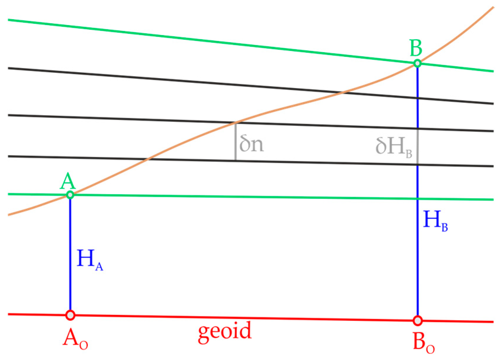
One of the height systems that fall into this group is the so-called geopotential numbers. To explain the need for their introduction, let us examine Figure 1, which illustrates the principle of geometric leveling in the real gravitational field where the sum of the leveled height differences between points $A$ and $B$ will not be equal to the difference between heights $H_A$ and $H_B$.

This is because the leveling increment $\delta n$ differs from the corresponding increment $\delta H_B$ of the $H_B$ height. As seen in Figure 1, it is caused by the non-parallelism of the level surfaces, which arises from the different distribution of mass density within the Earth’s interior. Therefore, in geometric leveling, gravity must also be measured at benchmarks, and the transition to geopotential heights must be made. If the potential difference between two points is denoted as $\delta W$, it can be expressed as follows [4]:

$$\mathsf{\delta }W=-\mathrm{g}\mathsf{\delta }\mathrm{n},$$

(1)

from which the next expression can be obtained:

$$W_B-W_A=-{\sum }_A^B\mathrm{g}\mathsf{\delta }\mathrm{n}.$$

(2)

The sum can be replaced with an integral, so Equation (2) becomes the following:

$$W_B-W_A=-{\int }_A^B\mathrm{g}\mathsf{\delta }\mathrm{n},$$

(3)

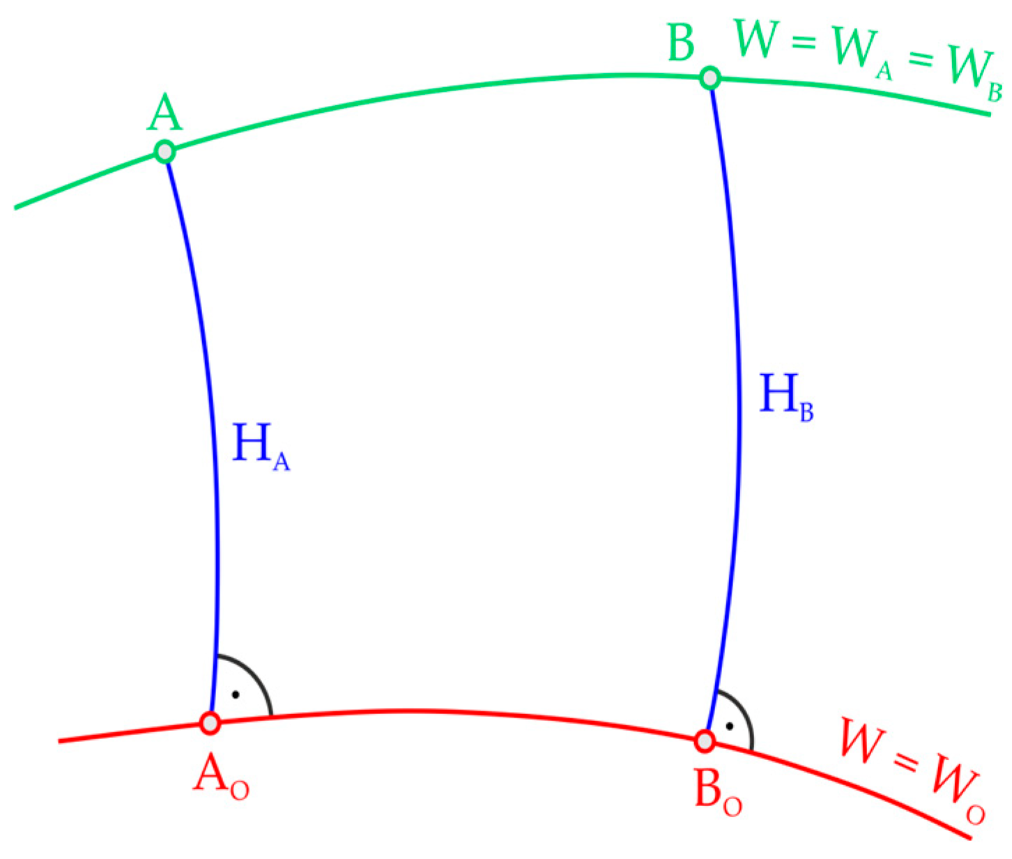
where the integral is independent of the integration path, so different leveling lines from $A$ to $B$ should give the same result. Point $O$ is located at sea level (on the geoid) and an arbitrary point $A$ on some different level surface is connected to point $O$ by geometric leveling in the real gravitational field (Figure 2).

According to Equation (3), the potential difference between points $O$ and $A$ is given by the following [4]:

$$W_O-W_A={\int }_O^A\mathrm{g}\mathsf{\delta }\mathrm{n}=C,$$

(4)

where $C$ represents the geopotential number of a given point and can be described as the difference between the Earth’s gravity potential at the observed point and potential on the reference geopotential surface. However, the use of geopotential numbers in practice is not very convenient because they do not have the dimension of height but are expressed in m²s⁻². For this reason, geopotential numbers are divided by different values of gravity for practical application, resulting in various height systems [2].

2.1.2. Dynamic Heights

Another type of height defined without assumptions about mass distribution is dynamic heights, which are obtained by dividing the geopotential number by the normal value of gravity on the ellipsoid surface at ellipsoidal height $h=0$ and geodetic latitude $\phi =45°:$

$$H^{DYN}= {\displaystyle \frac{C}{{\gamma }_0^{45}}}.$$

(5)

This value is constant for a given ellipsoid and is calculated using the expression of Somigliana [5]:

$${\gamma }_0= {\displaystyle \frac{a{\gamma }_a{cos}^2\phi +b{\gamma }_b{sin}^2\phi }{\sqrt{a^2{cos}^2\phi +b^2{sin}^2\phi }}},$$

(6)

where $a$ and $b$ are the semimajor and semiminor axes of the used level-ellipsoid, ${\gamma }_a$ the normal gravity at the equator, ${\gamma }_b$ the normal gravity at the pole, and $\phi$ the geodetic latitude. The value of normal gravity ${\gamma }_0$ is expressed in $\mathrm{m}{\mathrm{s}}^{-2}$, provided that ${\gamma }_a$ and ${\gamma }_b$ are also expressed in the same unit. The consequence of dividing the geopotential number by a constant is that dynamic heights have the dimension of height but not the character of height, as they represent purely a physical quantity, specifically the potential relative to the geoid, expressed in units of meters [4].

In Figure 3, points $A$ and $B$ lie on the same level surface, which implies that they have the same geopotential numbers and, consequently, the same dynamic heights, even though due to the non-parallelism of the level surfaces, they are not equally distant from the geoid.

It was previously stated that one of the methods for transitioning to a dynamic height system based on field measurements using geometric leveling is to convert the benchmark heights and height differences between them into the system of geopotential numbers. Then, dividing by the normal value of gravity on the ellipsoid surface at $h=0$ and $\phi =45°$, the dynamic height system is obtained. However, dynamic heights can also be obtained by converting the benchmarks into dynamic heights and correcting the height differences obtained from geometric leveling with a dynamic correction (DC), resulting in dynamic height differences. Then, through adjustment, the dynamic heights of all the points in the network are determined without transitioning to the system of geopotential numbers. The expression for calculating dynamic correction is as follows [4]:

$${DC}_{AB}= {\sum }_A^B{\displaystyle \frac{g-{\gamma }_0^{45}}{{\gamma }_0^{45}}}\delta n,$$

(7)

where g denotes the mean value of gravity between the start and the end point of the leveling line and $\delta n$ is the leveled height difference.

The dynamic height difference is obtained using Equation (7):

$$\mathit{\Delta }{H}_{AB}^{DYN}= \Delta n_{AB}+{DC}_{AB}.$$

(8)

where $\mathit{\Delta }{n}_{AB}$ denotes the sum of leveled height differences between $A$ and $B$.

2.2. Physically Defined Height

2.2.1. Orthometric Heights

Orthometric height is the curved-line distance measured along the plumbline (Earth’s gravity field line) from the geoid to the point of interest. It can be determined by dividing the geopotential number by the integral mean value of gravity for all the points along the plumbline $\overline{g}$ [2,4]:

$$H^{ORT}= {\displaystyle \frac{C}{\overline{g}}}.$$

(9)

This means that to define the orthometric height, we would have to measure gravity at every point along the plumbline (Figure 4), which is, of course, impossible, so the true orthometric height system cannot be achieved.

Since the integral mean value of gravity cannot be measured or calculated, because it requires a detailed model of mass distribution in the area of interest, it is determined based on a hypothesis about the distribution of mass within the Earth. Throughout history, proposals for determining this value have been made by Helmert, Niethammer, Mader, Müller, Ledersteger, and Ramsayer. Most countries that are using orthometric height systems today rely on Helmert’s approximation, which, for the normal density of Earth’s masses $\rho =2670 \mathrm{k}\mathrm{g} {\mathrm{m}}^{-3}$, can be calculated by the following [6]:

$$\overline{g}=g+0.0424 · {10}^{-5}H.$$

(10)

where $\overline{g}$ is expressed in $\mathrm{m}{\mathrm{s}}^{-2}$, provided that $g$ is given in the same unit and $H$ in meters.

Thus, when discussing geometric leveling, if we want to obtain orthometric heights for all the benchmarks in the leveling line, one method is to first convert the heights of the benchmarks and height differences into the geopotential number system. Then, in the geopotential number system, we perform an adjustment of the leveling line, which yields the geopotential numbers for all the points in the line. Finally, the transition to the orthometric height system needs to be made using Equations (7) and (8).

Another method for obtaining orthometric heights based on geometric leveling measurements is by applying the following orthometric correction [4]:

$${OC}_{AB}= {\sum }_A^B{\displaystyle \frac{g-{\gamma }_0^{45}}{{\gamma }_0^{45}}}\delta n+{\displaystyle \frac{{\overline{g}}_A-{\gamma }_0^{45}}{{\gamma }_0^{45}}}{H}_A- {\displaystyle \frac{{\overline{g}}_B-{\gamma }_0^{45}}{{\gamma }_0^{45}}}{H}_B$$

(11)

on the measured height differences:

$$\mathit{\Delta }{H}_{AB}^{ORT}= \Delta n_{AB}+{OC}_{AB},$$

(12)

resulting in orthometric height differences. By performing a least square adjustment using the obtained orthometric height differences, the orthometric heights of all points in the leveling line can be determined.

2.2.2. Normal Heights

The normal height system was developed in 1945 by Molodensky to circumvent the problem of determining the integral mean value of actual gravity along the plumbline [2,7]. This is achieved by using an approximate gravity field that can be precisely calculated at any point. For this purpose, the normal gravity field is used which represents the gravity field of an Earth-like ellipsoid [1].

To geometrically define normal heights, consider point A on the physical surface of the Earth (Figure 5).

This point has a certain potential $W$ and a normal potential $U$, where W_A ≠ U_A. If a point $B$ is now defined on the plumbline of point $A$ such that W_A = U_B, meaning the normal potential at point $B$ equals the real potential at point $A$, then the normal height of point $A$ can be defined as the geometric distance of point $B$ from the ellipsoid [4]. The surface on which point $B$ is located is called a telluroid and represents an approximation of the Earth’s surface. It is defined as a surface whose height above the ellipsoid corresponds to the height of the Earth’s physical surface above the quasigeoid. The reason for introducing the quasigeoid is that the distance from the ellipsoid to the quasigeoid, known as the height anomaly $\zeta$, can theoretically be calculated exactly, unlike the geoid, where this is not the case [8].

However, normal heights have a disadvantage compared to orthometric heights, which is the lack of physical meaning, as their reference surface is the quasigeoid rather than the geoid. The difference between those two surfaces is highly correlated with the height of the terrain, where the largest differences occur in high mountains, and at sea level there is no difference [8,9].

In mathematical terms, normal heights can be determined by dividing geopotential numbers by the mean normal gravity $\overline{\gamma }$ along the plumbline [4]:

$$H^N= {\displaystyle \frac{C}{\overline{\gamma }}} ,$$

(13)

where mean normal gravity is given by the following:

$$\overline{\gamma }= {\gamma }_0\left[1-{\displaystyle \frac{1}{a}}\left(1+f+m-2f{sin}^2\phi \right)H^N\right].$$

(14)

where $a$ denotes the semimajor axis of the used level-ellipsoid, $f$ the flattening of the level-ellipsoid, and constant $m={\omega }^2{a}^{2}b{G}^{-1}{M}^{-1}$ (where $\omega$ is the angular velocity of the selected level-ellipsoid which is equal to the angular velocity of the Earth, $b$ is the semiminor axis of the selected level-ellipsoid, $G$ is the universal gravity constant, and $M$ is the mass of the selected level-ellipsoid which is equal to the mass of the Earth). The resulting value of mean normal gravity $\overline{\gamma }$ is expressed in $\mathrm{m}{\mathrm{s}}^{-2}$.

Equations (13) and (14) depend on each other, meaning that normal heights cannot be determined directly, but iteration is required. In the iterative process, the initial value of normal height is set to zero, so $\overline{\gamma }$ is equal to ${\gamma }_0$, which is then used to calculate the new value of normal height. Then, new values of $\overline{\gamma }$ and $H^N$ are calculated until the new value and the previous value of the normal height in the iteration are equal.

As with dynamic and orthometric heights, normal heights can also be determined through the correction of height differences [4]:

$$\mathit{\Delta }{H}_{AB}^N= \mathit{\Delta }{n}_{AB}+{NC}_{AB},$$

(15)

which, in this case, is called the normal correction (NC) and is obtained using the following expression:

$${NC}_{AB}= \sum _A^B{\displaystyle \frac{g-{\gamma }_0}{{\gamma }_0}}\delta n+{\displaystyle \frac{{\overline{\gamma }}_A-{\gamma }_0}{{\gamma }_0}}{H}_A^N- {\displaystyle \frac{{\overline{\gamma }}_B-{\gamma }_0}{{\gamma }_0}}{H}_B^N.$$

(16)

2.2.3. Normal–Orthometric Heights

Both orthometric and normal height systems rely on actual gravity measurements along the leveling lines to calculate geopotential numbers or apply orthometric or normal correction. However, before the 1950s, the lack of precise gravimeters and extensive field gravity measurements led to the development and adoption of the normal–orthometric height system as an alternative.

The primary advantage of this height system is that it eliminates the need for direct gravity measurements. It uses the normal gravity field as a substitute for the Earth’s real gravity field to compute all gravity-related parameters. Instead of actual geopotential numbers $C$, differences in the corresponding normal potential (referred to as spheropotential numbers $C^{*}$) are used, and real gravity is replaced by normal gravity:

$$H^{NO}= {\displaystyle \frac{C^{*}}{\overline{\gamma }}}= {\displaystyle \frac{U_0-U}{\overline{\gamma }}},$$

(17)

where $U_0$ is the normal potential on the surface of the ellipsoid, $U$ is the normal potential of the level surface and $\overline{\gamma }$ is given by Equation (12).

However, normal–orthometric heights cannot be determined in practice using this equation because the value of $C^{*}$ cannot be obtained. For this reason, the values of normal–orthometric heights, based on geometric leveling measurements, are exclusively derived through the correction of height differences. The correction of height differences for obtaining normal–orthometric heights is called the normal–orthometric correction (NOC), and the method for its determination is presented below.

According to Bilajbegović [10], for two adjacent level surfaces (Figure 6) in the normal gravity field, the following applies:

$$U_0-U=\overline{\gamma } H=constant,$$

(18)

which, through differentiation, becomes the following:

$$d\overline{\gamma } H+\overline{\gamma }dH=0 \to dH=-{\displaystyle \frac{d\overline{\gamma }}{\overline{\gamma }}}H.$$

(19)

To determine Equation (19), it is necessary to introduce an approximation ${\displaystyle \frac{d\overline{\gamma }}{\overline{\gamma }}} \cong {\displaystyle \frac{d{\gamma }_0}{{\gamma }_0}}$ and calculate the normal gravity for the required ellipsoid. In general, the equation for normal gravity is as follows [4,10,11]:

$${\gamma }_0= {\gamma }_e\left(1+\beta {sin}^2\phi +{\beta }_1{sin}^{2}2\phi \right),$$

(20)

where $\beta$ is the global normal flattening, obtained using the following equation:

$$\beta = {\displaystyle \frac{{\gamma }_p-{\gamma }_e}{{\gamma }_e}}$$

(21)

where ${\gamma }_e$ and ${\gamma }_p$ are the normal gravity at the equator and pole (${\gamma }_e=9.7803267715 \mathrm{m}{\mathrm{s}}^{-2}$ and ${\gamma }_p=9.8321863685 \mathrm{m}{\mathrm{s}}^{-2}$ for the GRS80 ellipsoid). If these two values are substituted into Equation (21), the global normal flattening value of the GRS80 ellipsoid is obtained, which equals $\beta =0.0053024401$.

The coefficient ${\beta }_1$ in Equation (20) can be calculated using the equation [11]:

$${\beta }_1={\displaystyle \frac{1}{8}}{f}^2-{\displaystyle \frac{5}{8}}fm,$$

(22)

where $f$ is the flattening of the ellipsoid and m is a constant for the selected ellipsoid ($f=0.0033528107$ and $m=0.0034677477$ for GRS80). If these two values are substituted into Equation (22), the value of the coefficient ${\beta }_1$ for the GRS80 ellipsoid is obtained, which equals ${\beta }_1=0.0000058615$, so Equation (20) can be written as follows:

$${\gamma }_0=9.7803267715\left(1+0.0053024401{sin}^2\phi -0.0000058615{sin}^{2}2\phi \right).$$

(23)

Up to this point, the equations have described the general case for the GRS80 ellipsoid. In the following steps, values specific to the study area are introduced. By applying the trigonometric identity for the double angle and introducing the average geodetic latitude of all the benchmarks included in the study ($\phi =45°{52}^{\prime }{58}^{″}$), the equation for normal gravity acceleration for the GRS80 ellipsoid in the measurement area becomes the following:

$${\gamma }_0= 9.7803267715\left(1+0.0052910783{sin}^2\phi \right).$$

(24)

Differentiating Equation (24) gives the following:

$$d{\gamma }_0= 9.7803267715\left(0.0052910783\sin 2\phi d\phi \right),$$

(25)

and considering the approximation ${\displaystyle \frac{d\overline{\gamma }}{\overline{\gamma }}} \cong {\displaystyle \frac{d{\gamma }_0}{{\gamma }_0}}$, it follows that

$${\displaystyle \frac{d\overline{\gamma }}{\overline{\gamma }}}\cong {\displaystyle \frac{9.7803267715\left(0.0052910783\sin 2\phi d\phi \right)}{9.7803267715\left(1+0.0052910783{sin}^2\phi \right)}}.$$

(26)

Finally, if the value of the mean geodetic latitude for the measurement area ($\phi =45°52\prime 58″$) is substituted into the part of the denominator of Equation (26) (expression ${sin}^2\phi$), the following is obtained:

$${\displaystyle \frac{d\overline{\gamma }}{\overline{\gamma }}}=\left(0.0052766885\sin 2\phi d\phi \right),$$

(27)

and if Equation (27) is substituted into Equation (19), the expression for calculating the normal–orthometric correction for the area of interest is obtained as follows:

$${NOC}_{AB}=-0.0052766885\sin 2\phi d\phi H.$$

(28)

For practical calculations, if Equation (26) is divided by $\mathit{\rho }˝$ = 206264.806” (to normalize the units), Equation (28) can be written as follows:

$${NOC}_{AB}=-0.00000002558211\sin 2{\phi }_s{∆\phi }^{″}{H}_s,$$

(29)

where ${\phi }_s= {\displaystyle \frac{{\phi }_A+{\phi }_B}{2}}$, $∆{\phi }^{″}={\phi }_B^{″}-{\phi }_A^{″}$ in seconds, and $H_s= {\displaystyle \frac{H_A+H_B}{2}}$ in meters. The obtained normal–orthometric correction is in millimeters. The normal–orthometric height difference is obtained using the following equation [10]:

$$\mathit{\Delta }{H}_{AB}^{NO}= \mathit{\Delta }{n}_{AB}+{NOC}_{AB}.$$

(30)

The Republic of Croatia officially uses the normal–orthometric height system as its national vertical reference. On 4 August 2004, the Government of the Republic of Croatia brought the Decree on establishing new official geodetic data and map projections of the Republic of Croatia [12]. According to the Decree, Croatia adopted a new vertical reference system called HVRS71. HVRS71 was realized with the Second High Accuracy Leveling (cro. II. Nivelman visoke točnosti—IINVT) network of benchmarks with normal–orthometric heights. IINVT was stretched over the territory of former Yugoslavia (Figure 7). Mean sea level was determined by measurements at five tide gauges on the eastern shore of the Adriatic Sea: Koper (Slovenia), Rovinj, Bakar, Split, and Dubrovnik for a period of 18.6 years (Figure 7). More about HVRS71 can be found in Klak et al. [13], Rožić [14], Rožić and Razumović [15], and Pavasović et al. [16].

3. Leveling Survey

Precise leveling is a fundamental geodetic method used to determine height differences between points with high accuracy. In this approach, known elevations of the initial and final benchmarks serve as a reference for calculating the elevations of newly established benchmarks along the route. By measuring the height differences between successive benchmarks, it is possible to systematically determine the elevations of all the intermediate points. For the survey conducted on Medvednica Mountain, the initial and final benchmark heights were used as a basis for establishing a series of new benchmarks along the road Sljeme.

To achieve this, it was first necessary to establish the benchmarks and measure their coordinates using the GNSS method, as these benchmarks’ heights would be determined through precise leveling.

3.1. Benchmarks Coordinates

The points were located at distances 200 to 500 m apart depending on the openness of the horizon and tree canopies, all with the aim of better determining positions and minimizing interference during GNSS surveying. The points were measured three times, each for 30 s. One repetition consists of three consecutive measurements, with each measurement lasting 30 s, representing 30 measurement epochs. A total of 40 benchmarks were established along the trajectory (Figure 8).

The coordinates of all the points in the leveling line were stabilized with a steel bolt and determined by GNSS using the real-time high-precise positioning service of the Croatian Positioning System (CROPOS VPPS) [18,19,20]. By using the CROPOS VPPS service, plane coordinates (E, N) in the HTRS96/TM (EPSG:3765) map projection and normal–orthometric height in HVRS71 were obtained.

Along with HVRS71, based on the Decree on establishing new official geodetic data and map projections of the Republic of Croatia on 4 August 2004 [12], the Republic of Croatia established new official geodetic data and map projections of the Republic of Croatia. According to the Decree, a new horizontal reference system called the Croatian Terrestrial Reference System 1996 (HTRS96) was introduced based on the European Terrestrial Reference System 1989 (ETRS89) [21] with GRS80 as the reference ellipsoid.

In addition to the coordinates of the 40 newly stabilized benchmarks measured using the GNSS method, the coordinates of one gravimetric eccentric point, AGT03-E3, and three existing height benchmarks—two at the beginning and one at the end of the route—were required for this study. The coordinates of these points were obtained from the positional records compiled at the time of their stabilization.

3.2. Geomertric Leveling

Geometric leveling is a method for determining height differences between points, such as $A$ and $B$, with the leveling instrument and leveling staffs. By using horizontal sight, the leveling instrument, placed between two staffs, reads the sections on the two leveling staffs at points $A$ and $B$, thereby determining the height difference between these points (Figure 9) [22].

The height difference between points $A$ and $B$ is obtained as follows [23]:

$$\mathit{\Delta }h= l_B-l_A.$$

(31)

If the height of point $A$ is known, this difference is added to the known height to determine the height of point $B$.

Depending on the accuracy, geometric leveling can be divided into the following [24]:

• High accuracy leveling (cro. Nivelman visoke točnosti—NVT);
• Precise leveling (cro. Precizni nivelman—PN);
• Technical leveling with increased accuracy (cro. Tehnički nivelman povećane točnosti—TNPT);
• Technical leveling (cro. Tehnički nivelman—TN);
• City leveling (cro. Gradski nivelman—GN).

The characteristics of all of these can be found in

Table 1. Characteristics of geometric leveling based on accuracy [24].

Leveling Network	Line Length [d]	Accuracy [U0]
NVT	$\le$300 km	$\pm$$1.0 \mathrm{mm}\surd$km
PN	$\le$80 km	$\pm$$2.0 \mathrm{mm}\surd$km
TNPT	$\le$50 km	$\pm$$5.0 \mathrm{mm}\surd$km
TN	$\le$30 km	$\pm$$8.0 \mathrm{mm}\surd$km
GN	-	$\pm$$2.0 \mathrm{mm}\surd$km

.

3.2.1. ISO Standard Test

In this paper, leveling measurements were carried out using the precise leveling method with two leveling instruments—Leica DNA03. One of the level instruments is owned by the Chair of State Survey, while the other belongs to the Chair of Engineering Geodesy of the University of Zagreb, Faculty of Geodesy (will be referred to as SS and EG instrument throughout the article). Prior to the measurements, both the leveling instruments and leveling staffs were tested in accordance with the ISO standard HRN ISO 17123-2:2004 for testing geodetic instruments and measuring equipment [25]. The testing procedure was carried out by placing two leveling staff 60 m apart, with the leveling instrument positioned in the middle between them. Two sets of measurements were performed. The first set of measurements consisted of 20 pairs of readings, where each pair included two readings: a backsight reading on staff at point $A$ and a foresight reading on staff at point $B$. Between each pair of readings, the height and position of the level were slightly adjusted. After the first 10 pairs of readings, the order of backsight and foresight readings was reversed, and the remaining 10 pairs of readings were performed. For the second set of measurements, the staff at points $A$ and $B$ switched places. The entire measurement procedure was carried out in the same manner as in the first set [26].

After completing the measurements according to the specified procedure, statistical tests were conducted to confirm the following hypothesis [26]:

• The calculated empirical standard deviation per km double run (s_i) is smaller than the corresponding value σ declared by the instrument manufacturer;
• Two empirical standard deviations per km double run (s_i and ${\tilde{s}}_{\mathrm{i}}$ determined from two different measurement series belong to the same pattern;
• The difference (δ) of the staff zero errors for a pair of leveling staffs is smaller than 0.64 s, where s is the empirical standard deviation.

The results of the test conducted are presented in

Table 2. Results of the ISO standard test for two leveling instruments.

Hypothesis	Allowable Value [mm]	SS Instrument Value [mm]	EG Instrument Value [mm]
1	0.30	0.29	0.22
2	0.52 < x < 1.91	1.74	0.58
3	0.050	0.015	0.010

, where the maximum allowable error for each hypothesis is given, along with the values obtained using the leveling instruments. The results of the testing show that both instruments are accurate and meet the required precision for measurements in precise leveling, and it is possible to begin fieldwork.

3.2.2. Precise Leveling Measurements

Precise leveling measurements began on 12 October 2023, at the base of Mount Medvednica, specifically near the Sljeme tunnel, where two benchmarks (626_II_309L and 626_II_309D) are located at the entrance. The leveling traverse was carried out starting from those initial benchmarks, extending all the way to the final benchmark (626_II_24) near the Stara Lugarnica restaurant at the summit of Medvednica. The purpose of this work was to determine the heights of the newly established benchmarks (R1–R39). The positional coordinates of the initial and final benchmarks in HTRS96 as well as heights in HVRS71 are known from the positional descriptions.

The first step of each day’s measurements involved testing the main condition of the level by performing leveling from the middle and the end. The leveling was conducted simultaneously using two digital leveling instruments, with concurrent readings taken on two invar three-meter staffs (Figure 10).

During the measurements, care was taken to ensure the levels were positioned at the midpoint between the leveling staffs. The leveling was performed in both directions (forward and backward) by closing loops between all the adjacent benchmarks. For example, the first line was measured from benchmark 626_II_309L to R1 and then back to 626_II_309L, continuing in this manner up to the final benchmark. For each line, the discrepancies of double measurements for both instruments were calculated and compared to the allowable discrepancy value for that line (Appendix A.1) to verify measurement accuracy.

The total length of the leveling line in one direction is 12.5 km, starting from the Sljeme tunnel near the Sljeme cable car and extending to the Stara Lugarnica restaurant. The height of the starting benchmark 309 L, according to the official position description of the Croatian State Geodetic Administration, is 279.4281 m, while the height of the final benchmark is 912.8089 m. This means that the official height difference between the two benchmarks is 633.3808 m.

Table 1 provides the allowable leveling error in precise leveling ($U_0$), which amounts to $\pm$2.0 mm$\surd$km, and considering that the leveling line is approximately 12.5 km long, the closure accuracy of the line is $\pm$7 mm. To obtain the probable error of double height difference measurement at the leveling length of 1 km for the leveling line in this article, the following equations should be applied [27]:

$$u_{oD}= {\displaystyle \frac{2}{3}}{m}_{oD}.$$

(32)

In Equation (32), $m_{oD}$ represents the mean square error of double measurements of height differences at the leveling length of 1 km [27]:

$$m_{oD}= \pm {\displaystyle \frac{1}{2}}\sqrt{{\displaystyle \frac{{\mathit{d}}^T\mathit{P}\mathit{d}}{n}}},$$

(33)

where $\mathit{d}$ is the discrepancy vector of double measurements of leveling side height differences, $\mathit{P}$ is the weight matrix, and $n$ is the total number of leveling sides in leveling line.

Table 3. Statistics and accuracy of leveling line (leveling length, d [km]; total height difference, Δh [m]; mean square error of double measurements of height differences at the leveling length of 1 km, m_oD [mm]; probable error of double height difference measurements at the leveling length of 1 km, u_oD [mm]; and probable error of double height difference measurements of complete leveling length), u₀ [mm].

Value	SS	EG
d [km]	12.5	12.5
Δh [m]	633.3911	633.3907
moD [mm]	0.30	0.37
uoD [mm]	0.20	0.25
u0 [mm]	2.50	3.13

provides data on the leveling line, such as the line length, total height difference, values of $m_{oD}$ and $u_{oD}$ for both leveling instruments for a length of 1 km, and the value of $u_0$ for the total leveling length. Considering that it was stated above that the maximum allowable error is ±7 mm, the obtained error is within the allowable limit.

As seen in the table, the probable error of double height difference measurements of complete leveling length for both instruments is less than the previously defined maximum of 7 mm, indicating that the measurements were successfully conducted.

4. Gravity Measurements

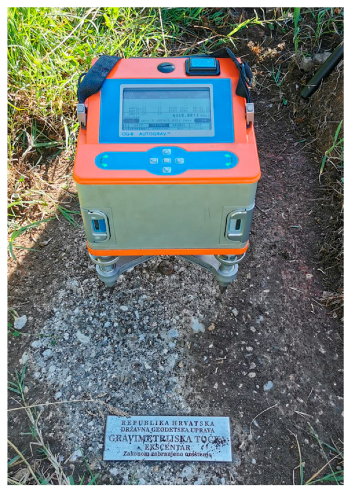
The gravimetric survey of all benchmarks in the leveling line was conducted on 15, 22, and 24 July 2023, using the Scintrex CG-6 relative gravimeter. Since the measurements were performed using relative gravimetry, it was necessary to select a reference point with a known absolute gravity value to determine the values at other points relative to it. As the absolute reference point, an eccentric point of one of Croatia’s absolute gravity stations was selected, located on Medvednica (AGT03—E3), whose gravity acceleration value is known (Figure 11).

The measurements were conducted in such a way that the relative gravity acceleration of the absolute point was measured multiple times throughout the day, while the gravity acceleration values of the remaining points were measured once between these measurements. The measurements at the absolute point were repeated to successfully eliminate the gravimeter drift from the results.

4.1. Corrections of Gravity Measurements

After measurements have been completed, all relative gravity values need to be corrected for certain adjustments that affect the measured gravity. These corrections can be divided into two main groups [28]:

• Corrections related to the measuring instrument;
• Corrections related to the Earth’s geophysical processes.

4.1.1. Corrections Related to the Measuring Instrument

Corrections related to the measuring instrument include the following:

• Correction for the air pressure

The redistribution of air masses in the Earth’s atmosphere causes constant variations in gravity. Gravity and air pressure are inversely proportional, meaning that as air pressure increases, gravity decreases. The correction for gravity due to the influence of air pressure, expressed in mGal (i.e., ${10}^{-5}\mathrm{m}{\mathrm{s}}^{-2}$), is calculated using the following equation [28,29]:

$$g_{ap}=\alpha \left(p_m-p_0\right),$$

(34)

where $\alpha$ is the barometric admittance factor for Central Europe with a value of $0.0003 \mathrm{m}\mathrm{G}\mathrm{a}\mathrm{l}/\mathrm{h}\mathrm{P}\mathrm{a}$, $p_m$ the air pressure measured at the moment of gravimetric measurement in hPa, and $p_0$ the mean long-term air pressure at the height ($H$) of the gravimetric point in hPa which can be obtained by the following equation:

$$p_0=1013.25{\left(1-{\displaystyle \frac{0.0065H}{288.15}}\right)}^{5.2559};$$

(35)

• Correction for Earth’s polar motion

Daily or secular variations in the dynamics of Earth’s rotation are caused by the redistribution of Earth’s masses due to geophysical processes and gravitational influences from celestial bodies. The result of this is a change in the position of Earth’s pole relative to the celestial pole, which manifests as a variation in gravity. The correction to eliminate this variation can be calculated using the following equation [28,29,30]:

$$g_{epm}=-\delta {\omega }^{2}a\sin \phi \cos \phi \left(x_t\cos \lambda -y_t\sin \lambda \right)·{10}^5,$$

(36)

where $\delta$ is the gravimetric factor, which represents the ratio of the actual to the theoretical change in gravity, and for the approximation of Earth as a perfectly elastic sphere, it has a value of $1.164$; $\omega$ is the angular velocity of Earth’s rotation ($\omega =7.2921159·{10}^{-5} \mathrm{r}\mathrm{a}\mathrm{d} {\mathrm{s}}^{-1}$), a is the equatorial radius of Earth ($a=6378136.6 \mathrm{m}$), $\phi$ and $\lambda$ are the geodetic latitude and longitude of the measurement point, and $x_t$ and $y_t$ are the pole coordinates at the moment of gravity measurement. In Equation (36), $g_{epm}$ is expressed in mGal. The values of pole coordinates at midnight of every day are provided by IERS [31], and with linear interpolation, pole coordinates at the moment of gravity measurement can be calculated.

• Correction for the Earth’s tides.

The correction for the influence of Earth’s tides needs to be made due to the error in the measured gravity acceleration caused by the gravitational effects of celestial bodies on Earth. The Sun and the Moon have, by far, the greatest influence of all celestial bodies, so the influence of other celestial bodies can be neglected. The correction for the influence of Earth’s tides can be calculated using the following equation [32]:

$$g_{et}=\delta \left(g_s+g_m\right),$$

(37)

where $\delta$ is the gravimetric factor, $g_s$ component of the Moon’s influence on Earth’s tides, and $g_m$ component of the Sun’s influence on Earth’s tides. These two components can be calculated using the Longman model for the calculation of Earth’s tides [29,32]. Although the Scintrex CG-6 instrument has the capability to automatically calculate Earth’s tidal waves, in this study, raw gravity values were used, and the correction for tide influence was calculated using the Longman model. In Equation (37), $g_{et}$ is expressed in mGal.

4.1.2. Corrections Related to the Earth’s Geophysical Processes

Corrections related to the Earth’s geophysical processes include the following:

• Correction for the height of the measuring sensor

When conducting gravimetric measurements at a given point, the gravimeter measures the gravity value at the height of its sensor. However, in practice, this measured value is not directly useful, as the required value is gravity at the actual point, i.e., on the physical surface of the Earth. To obtain the gravity value at the Earth’s surface, it is necessary to determine how gravity changes with height variation and to measure the distance between the instrument’s sensor and the physical surface of the Earth at the time of measurement.

The change in gravity with height variation is called the vertical gradient, and the value used in practice is 0.3086 mGal/m. The height of the measurement sensor relative to the physical surface of the Earth cannot be directly determined, as the sensor is enclosed within the instrument’s housing. For this reason, the manufacturer specifies in the user manual the distance between the measuring sensor and the lower edge of the instrument. The user must then measure the distance from the Earth’s surface to the lower edge of the instrument in the field, based on which the correction for the sensor height in mGal can be calculated using the following equation [4,28,29]:

$$g_{hms}=0.3086\left(h_m+h_0\right),$$

(38)

where $h_m$ is the height from the Earth’s surface to the lower edge of the instrument measured in the field and $h_0$ the height between the measuring sensor and the lower edge of the instrument given by the manufacturer (for Scintrex CG-6, $h_0=0.066 \mathrm{m}$ [33]).

• Correction for the tilt of the measuring sensor

For the gravimeter to accurately determine the gravity value, the equipotential surface on which the measuring sensor is located must be parallel to the equipotential surface at the point of interest. If these two surfaces are not parallel, the measurement will not be entirely correct. The tilt of the gravimeter relative to its ideal position can be considered in relation to two axes ($x$ and $y$) and can be denoted as ${\theta }_x$ and ${\theta }_y$. The correction for the tilt of the measuring sensor can then be calculated using the following equation [34]:

$$g_{tms}=g_m\left(1-\cos {\theta }_x\cos {\theta }_y\right),$$

(39)

where $g_m$ is the measured gravity value at the point. Since the gravimeter must be precisely leveled before measurement, the ${\theta }_x$ and ${\theta }_y$ values are always very small, expressed in arcseconds. As a result, this correction will always be very minor and practically negligible.

• Correction for gravimeter drift

Due to the imperfections of the measurement system during field surveys, the gravimeter’s spring undergoes a time-dependent variation from its initial equilibrium position. This variation is called gravimeter drift, and to obtain a correct gravity value, it must be eliminated. While the order of other corrections is not crucial, the gravimeter drift correction must always be applied last to ensure that only the time-dependent changes in the spring’s zero position are modeled. A necessary condition for drift elimination is that at least one point is observed at least twice within a single day [28]. If this condition is met, the drift correction can be calculated in three steps (Figure 12):

• From the measurement day, the gravity values of the point that was observed multiple times that day (in this case, point AGT03-E3) need to be extracted, with all the previously mentioned corrections already applied (black circles);
• A gravimeter drift model is created based on the extracted gravity values and their corresponding measurement times. In this article, the method of linear regression is used for this purpose, resulting in a drift model, i.e., the coefficients of the equation of the line that best approximates all the measurements (red line);
• Based on the drift model, it is necessary to calculate the gravimeter drift value for each point in a day and correct the gravity measurements accordingly (blue circles).

In

Table 4. Numerical procedure of gravimeter drift correction.

Measuring Day	Δ(n − 1) [mGal]	Model	Δd(n − 1) [mGal]
15 July 2023	0.078	$y=0.000005x+4343.606$	0.001
22 July 2023	−0.042	$y=-0.000001x+4343.849$	0.006
24 July 2023	−0.013	$y=-0.000001x+4343.872$	0.002

, the procedure for the numerical correction of the gravimeter drift is presented. The first column shows the difference between the first and last gravity acceleration values of a repeatedly observed point in a day. The second column contains the gravimeter drift model, i.e., the equation of the trendline that best describes the measurements. The third column displays the differences between the first and last gravity acceleration values of a repeatedly observed point in a day after applying the drift correction.

In Appendix A.2, a numerical example of gravimeter drift calculation for the first day of measurement is provided.

4.2. Adjustment of Gravity Measurements

After all the errors have been removed from the relative gravity measurements using the mentioned corrections, the network adjustment can begin to obtain absolute values of gravity at all the points. In this article, the adjustment was performed using the least squares method for indirect measurements, where the measurement functions were the measured gravity differences between points. Based on the measurement functions, the design matrix ($\mathit{A}$) and the observation vector ($\mathit{l}$) were created, while the weight matrix ($\mathit{P}$) was generated based on the mutual distances between the points. The adjustment was carried out using the Gauss–Markov model based on the least square’s method [35]:

$${\mathit{v}}^t\mathit{P}\mathit{v}=min,$$

(40)

Whose stochastic model includes the weight matrix and empirical part is defined by the following equation:

$$\mathit{v}=\mathit{A}\mathit{x}-\mathit{l}.$$

(41)

The result of the adjustment is the absolute gravity values for all the points in the leveling line. In accordance with the Regulation on the Confidentiality of Defense Data of the Republic of Croatia [36], gravimetric survey data must not be disclosed without authorization. Therefore, the absolute gravity values for all the points in the leveling line are not provided in this article. However, to illustrate the variation in gravity along the leveling line, Figure 13 presents a gravimetric map of the survey area, where the gravity values across the entire displayed region were obtained through Kriging interpolation.

5. Results and Discussion

Based on the leveling and gravimetric measurements described in Section 3 and Section 4, heights were calculated in all the height systems mentioned in Section 2. In all the systems, except for the normal–orthometric height system where this is not possible, the heights were determined using both the methods described in Section 2. Additionally, an adjustment of the leveling line was performed, providing height values without considering gravity (geometric heights), enabling an analysis of the impact of gravity on the different height systems. Since both instruments achieved satisfactory accuracy and the obtained values are nearly identical, for the simplicity of further presentations, the average values of the two instruments were taken for all the subsequent analyses.

Table 5. Analysis of height differences between heights obtained from geopotential numbers and those calculated with height difference corrections (in meters).

Statistics	Dynamic Heights	Orthometric Heights	Normal Heights
Min	0.0000	0.0000	0.0000
Max	0.0000	0.0000	0.0000
Median	0.0000	0.0000	0.0000
Average	0.0000	0.0000	0.0000

provides statistical data comparing the heights obtained by dividing geopotential numbers by the corresponding gravity value Equations (5), (9) and (13) with the heights derived using height difference corrections in different height systems (Equations (8), (12) and (15)).

The statistics indicate that no significant difference exists, meaning that, in practice, it does not matter which method is used to determine heights, as the results will be the same. However, for faster computation, if heights need to be determined in all the height systems, it is more convenient to use geopotential numbers, as only one adjustment is required. On the other hand, if heights are needed in a single height system, it is more practical to apply corrections to height differences and perform the adjustment within the corresponding height system.

To analyze the impact of gravity on different height systems, the geometric heights of points were calculated based on the adjustment of the geometric leveling without considering any gravity values. These resulting heights were then compared with orthometric (Figure 14a), normal (Figure 14b), and normal–orthometric (Figure 14c) heights to assess the contribution of the measured gravity acceleration to each height system. A comparison with dynamic heights was not performed because dynamic heights do not have the characteristics of true heights, and as such, this analysis does not carry significant meaning.

The first observation is that the differences between the geometric and normal–orthometric heights are very small, with slightly larger differences at higher elevations. The reason for this can be seen in Equation (29), and in the fact that the starting and ending benchmarks are defined in that height system. As shown in Equation (29), the calculation of the normal–orthometric correction does not depend on gravity but rather solely on the difference between the geodetic latitude and geometric height.

However, the impact of gravity is clearly visible at normal and orthometric heights. For orthometric heights, the difference from geometric heights reaches its maximum value at the points with the highest elevations, where this difference is around 3.7 cm. In the case of normal heights, the difference from geometric heights increases with elevation, reaching a value of 3 cm at the end of the leveling line. This clearly demonstrates the impact of the measured gravity on these height systems.

In Section 2.2.2, it is defined that the height difference between the geoid and the quasigeoid is correlated with the terrain elevation. Specifically, the difference between orthometric and normal heights is most pronounced in high-altitude regions, while at sea level, there is no difference at all. To verify this statement, the differences between the calculated normal and orthometric heights were determined at all the points along the leveling line (Figure 15).

The figure shows that the smallest differences occur at the beginning of the leveling line, where the elevation is the lowest. However, even there, a difference of approximately 4 mm is present since the starting point is at an elevation of around 300 m. In the second half of the leveling line, where elevations are higher, these differences increase, reaching values of up to 1 cm. As can be seen, the increase in these differences is not linear, although it might be assumed at first glance. The reason for this is that orthometric heights are determined under the assumption of mass distribution, where the mass density is taken as constant, while the actual mass distribution cannot be precisely determined. Additionally, the topography in the vicinity of the leveling line significantly affects gravimetric measurements, which can also contribute to the nonlinear increase in the differences between normal and orthometric heights. Nevertheless, the figure clearly shows a tendency for this difference to increase with elevation, thus practically confirming the theoretical claim.

Although the leveling measurements were performed with very high accuracy, the gravimetric data cannot be considered completely error-free. This is primarily because the measurements were taken during the day when vehicle traffic was present, which could introduce slight disturbances in the gravity measurements. Additionally, the influence of underground water was not accounted for, as no piezometers were available in the vicinity to measure groundwater levels. The eccentricity from which the absolute gravity value was obtained was observed nearly 25 years ago, which also introduces some uncertainty. These factors could affect the final gravity values at the leveling benchmarks. Therefore, while there may be some potential errors in the gravimetric data, these errors are minimized in relative gravimetry by subtracting the measurements from each other. As a result, the final gravimetric values should be sufficiently accurate, and the obtained heights can be reliably compared.

6. Conclusions

To determine different height systems based on geometric leveling measurements, there are two methods. One method involves transitioning to the system of geopotential heights and performing the adjustment in the geopotential height system, after which the desired height system is obtained by dividing the geopotential heights by the corresponding value of gravitational acceleration. The second method involves calculating the appropriate correction for the desired height system, which is then added to the measured height differences in the geometric leveling. This results in height differences in the desired height system, which can then be used for the adjustment to directly obtain the heights in the desired system. Using both methods will yield identical height values, meaning that it does not matter which method is used.

However, for both methods of determining heights, it is essential to measure the gravitational acceleration at the points whose heights we wish to determine. This article presents an analysis of the impact of measured gravitational acceleration in different height systems, showing how the measured gravitational acceleration can influence the determined height by several centimeters. This means that for highly precise works, measuring gravity is not only recommended but necessary to maintain centimeter-level accuracy in height determination.

Additionally, the article presents the relationship between orthometric and normal heights, specifically how these heights differ at certain elevations above sea level. While there is no difference at sea level, in mountainous regions, this difference is quite pronounced and can exceed values greater than 1 cm. These quantified results reinforce the theoretical understanding that gravity and elevation are intrinsically linked in height system realizations and provide a practical reference for future studies or operational implementations that aim to integrate gravimetric and leveling data in regions with significant elevation gradients.