Analytical Modeling of Particle Scratching Process

Abstract

This study develops a new physical and analytical model for the particle scratching process, where a particle is modeled as a sphere. It investigates the flow of workpiece material introduced by the particle’s motion, dividing the contact area into zones of elastic and plastic deformation. Forces applied to the particle in both zones are calculated, and parameters defining the extent of elastic rebound and plastic upheaval are introduced. The study also presents stress distribution in the plastic zone, discusses the factors influencing the force ratio, and reveals that the force ratio increases with greater elastic rebound, plastic upheaval, cutting depth, and strain strengthening, but decreases with larger particle sizes. Yield stress was found to have no effect on the force ratio. These findings will guide research in practical material processing as well as in scratch applications.

1. Introduction

The scratching process of particles is a complex material removal process involving cutting, plowing, and rubbing, and it widely exists in abrasive wear, abrasive machining, and other industry applications. Mechanisms of particle–workpiece interaction and material removal at the microscopic level are very important for the comprehensive understanding of abrasive wear, abrasive machining, and other industry applications. A number of cutting experiments with a single particle were performed to study the mechanism of particle–workpiece interaction [1]. The acting forces and the profile of the generated grooves were measured to analyze the effect of cutting speed, depth of cut [2], abrasive type [3], and particle geometry [4] on the process of material removal. The mechanical models of specific energy [5] and cutting forces [6] during particle cutting were proposed. Even the cutting forces of a single particle were integrated to predict the grinding forces [7]. The scratching test is a common test method for abrasive wear, including parallel scratches [8] and intersecting scratches [9].

Modeling is essential for understanding the particle scratch process. A scratching model of the Berkovich diamond indenter has been presented to predict the machined depth [10]. A material removal model has been established to estimate wear rate [11]. Chen et al. presented a model based on the theories of elastic–plastic micro-contact mechanics and abrasive wear mechanism to investigate the effect of particle deformation in chemical mechanical polishing [12]. Modeling of wear processes is the most important factor influencing wear. A model of abrasive has been given to link different effects together to better understand their influence [13]. A 3D numerical modeling has been established to determine contact pressure, normal and friction force, local friction of abrasive, and coefficient distribution [14]. The meshless smoothed particle hydrodynamics method has been used to establish numerical modeling of abrasive wear [15]. In the existing research, most analytical models are 2D models. Three-dimensional simulated models have been applied to the scratching process, but the method of simulation is difficult to achieve high accuracy and takes a long time, which is not convenient for investigating the physical phenomena of the scratching process.

In this study, physical and analytical models of the scratching process have been proposed. The particle is simplified as a sphere, and the direction of material flow and removal are considered. The contact zone is divided into the elastic deformation zone and the plastic deformation zone. In the elastic deformation zone, the calculation of contact stress follows the Hertz stress distribution. The flow stress in the plastic deformation zone is determined by the corresponding strain, and the strain is the function of the vertical distance from a specific location to the interface of elastic deformation and plastic deformation zone. Tangential and normal forces applied to the particle have been calculated by integrating contact or flow stress on the contact zone. The stress distribution on the plastic deformation zone according to the analytical model has also been given. The force ratio has been presented, and the parameters that may affect it have been discussed.

2. Physical Model and Analytical Model of Scratching Process

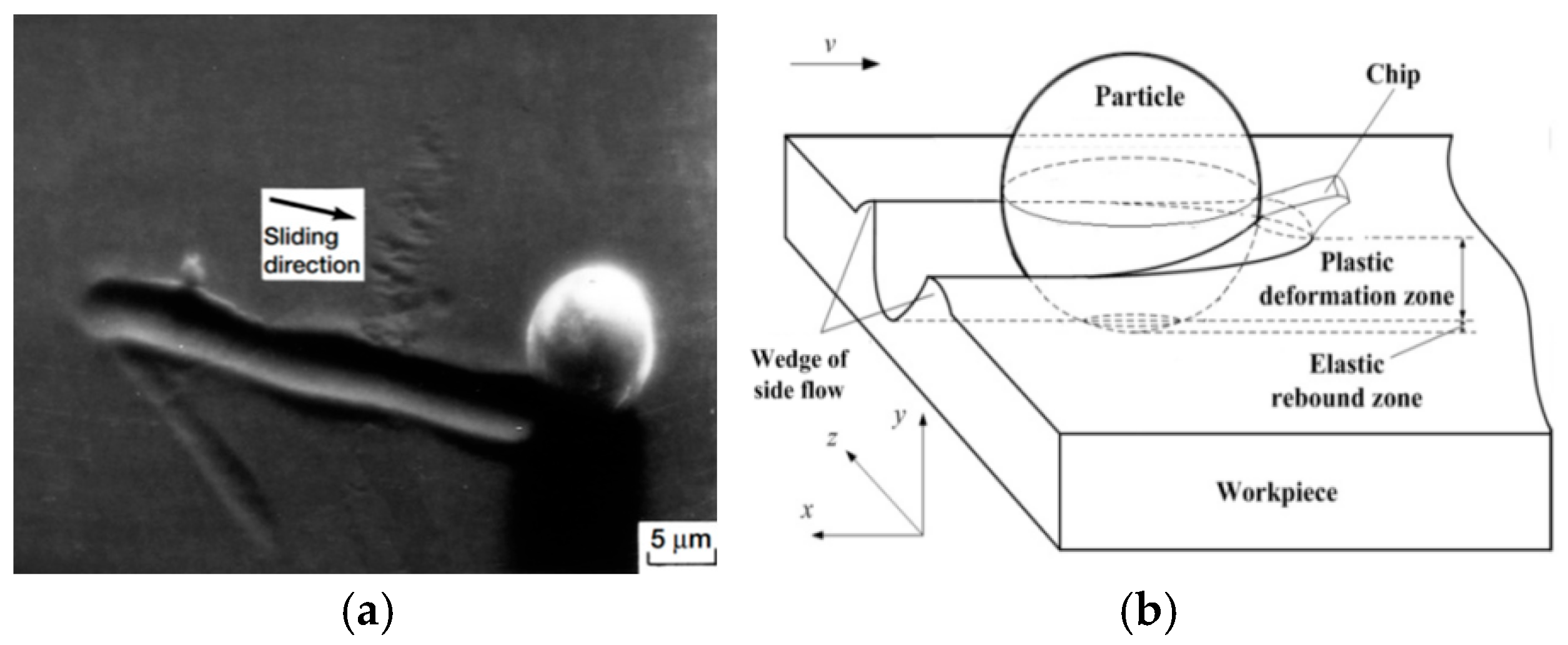
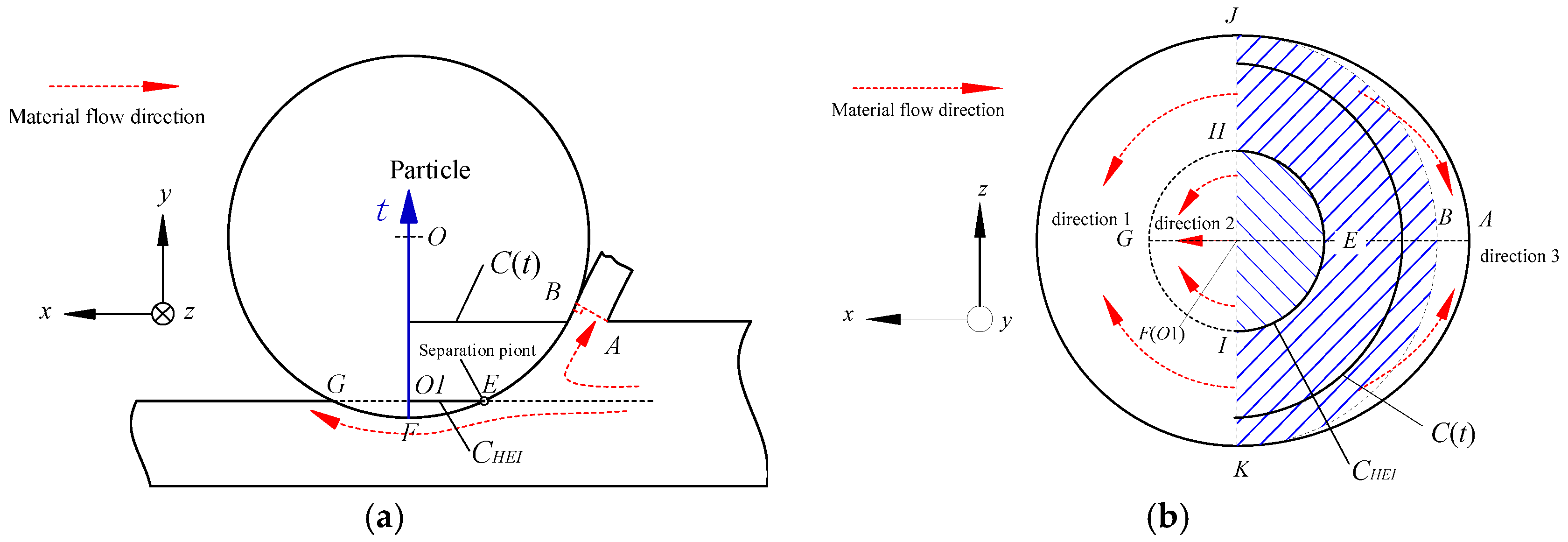
2.1. Physical Model

In this paper, a new physical and analytical model about particle scratching is proposed, in which the physical process and physical model are shown in Figure 1. The particle is simplified as a sphere. When the particle engages with the workpiece at an extremely small depth of cut, the work material undergoes elastic deformation. It is defined as the rubbing phase. With increasing depth of cut, plastic deformation occurs, and the work material piles up at the front and flows to the sides of the particle to form a groove. It is defined as the plowing phase. As the depth of cut continues to increase, the work material can no longer withstand the tearing stress, and a chip is formed. The chip formation stage is defined as the cutting phase. Therefore, there exist three types of material deformation in the single-particle cutting process, namely elastic deformation, wedge of side flow, and chips. However, the three types of material deformation may take place simultaneously.

As shown in Figure 2, direction 1 represents material flowing along the flank of the particle to ward the wedge, direction 2 represents material in zone F-HEGI flowing under the particle and rebounding back at point G behind the particle. Direction 3 represents the formation of chips. The separation point E is shown in the side view, which divides the contact zone into the plastic zone and the elastic zone.

The material in zone F-HEI deforms elastically. The maximum stress occurs at point F, and the value is almost equal to the yield stress σ_y of the material. The minimum stress occurs on the circumference of circle O₁, and the value is 0. As shown in Figure 2b, the material in the zone HEI-JBK deforms plastically.

In the zone HEI-JBK, the materials experience tensile stress along the particle surface and compressive stress perpendicular to the particle surface. In order to state the material flow clearly, the x-axis is built with its origin at the F point, and the positive direction is the same as the direction of the Y-axis. In any half-circular, the material was considered to flow from half-circular HEI along the surface of the particle, and the half-circular in a plane always perpendicular to the x-axis in the material flow process.

The plastic deformation of the material begins in the arc HIE and ends in the arc JLK. In the t coordinate, an arbitrary plane which is perpendicular to the t-axis intersects with the particle surface, and the intersection line is a half circle named C(t). It is obvious that the length of arc C(t) is a function of t. In particular, the half-circular was named the origin length of plastic deformation C_HEI when the plane through O₁ point, the half-circular was named the maximum length of plastic deformation C_JBK when the plane through the B point. The material flow and deformation process is compared to a circular rubber band set into a sphere in order to describe the flow and deformation process of the plastic deformation zone vividly. It is worth pointing out that only half of the circular rubber band contacts the sphere because the material contacts the particle with a part of the hemispherical surface. The initial contact position of the semicircle rubber band and sphere corresponds to C_HEI in the physical model. The arbitrary position of the semicircular rubber band corresponding to C(t) in the physical model. The tensile strain in plastic deformation can be calculated similarly to the tensile strain of a rubber band being stretched over a sphere. So, the tensile strain ε_t(t) can be expressed as:

$${\epsilon }_t\left(t\right)={\displaystyle \frac{\widehat{C\left(t\right)}-\widehat{C_{HEI}}}{\widehat{C_{HEI}}}}$$

(1)

The material is considered to be incompressible during plastic deformation, namely, the material volume is constant. The material can be assumed to suffer the plane strain condition. So the compress strain ε_c(t) under the t coordinate can be expressed as:

$${\epsilon }_c\left(t\right)={\displaystyle \frac{\widehat{C_{HEI}}}{\widehat{C\left(t\right)}}}-1$$

(2)

The forces during hard particle and surface interaction are generated from the compressive deformation of the workpiece material and the friction forces due to compression. So the dynamic mechanical properties of workpiece material under compression conditions need to be tested and used in the analysis of the two-body abrasive wear process.

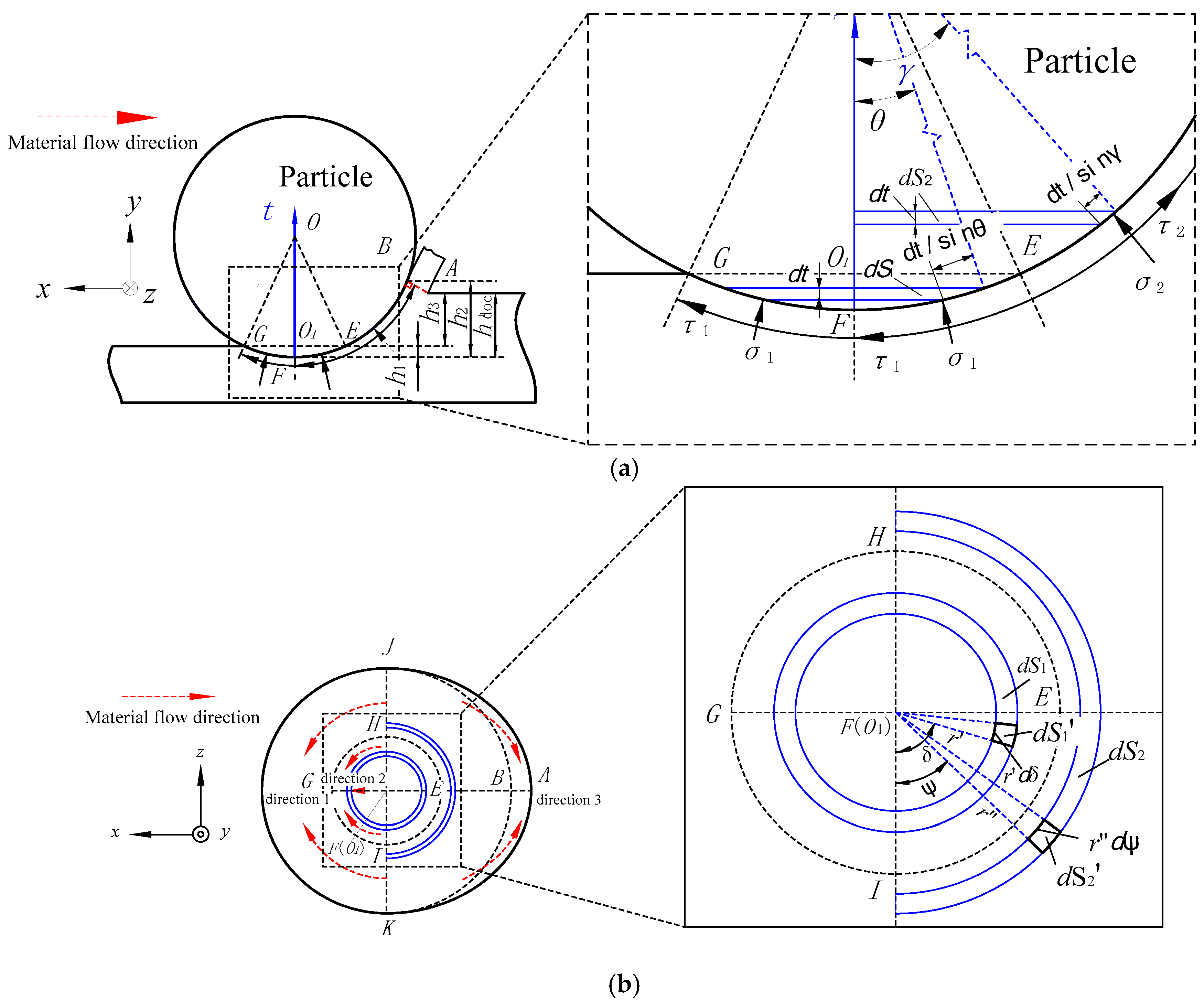
2.2. Analytical Model

Forces applied to the particle mainly come from material compressive stress and friction. The resultant forces in the Z direction are 0 due to the symmetrical particle geometry. There are two work-material deformation zones, namely, the elastic deformation zone F-HEIG and the plastic deformation zone HEI-JBK, which are mentioned in Section 2.1. The forces applied on the particle are obtained by integrating the compressive stress and friction stress on the surface of zone F-HEIG and zone HEI-JBK, respectively.

As shown in Figure 3a, compressive stress and shear stress produced by friction are applied to the abrasive surface. h_doc is the nominal depth of cut, h₁ is the rebound height, and h₂ is the wedge height of side flow. h₃ is the actual depth of the groove. h₃ is expressed as:

$$h_3=h_{doc}-h_1$$

(3)

In order to calculate the forces applied on the particle, the t-axis is built whose origin is the F point and the positive direction is the same as the direction of the Y-axis.

As shown in Figure 3b, in elastic deformation zone F-HEIG, the element of area dS₁’ can be expressed as:

$$d{S}_1^{\mathrm{\prime }}=r^{\mathrm{\prime }}\cdot dS\cdot \left({\displaystyle \genfrac{}{}{0pt}{}{dt}{\mathrm{s}\mathrm{i}\mathrm{n}\theta }}\right)$$

(4)

where r’ is the section-radius of the element in zone F-HEIG, which is perpendicular to the Y-axis, r’ = r·sinθ. θ is the included angle between line OO₁ and the line connecting point O and an arbitrary element in zone F-HEIG.

In element area dS₁, the force produced in the X direction and Y direction are expressed as:

$$d{F}_{X_{F-HEIG}}=4{\int }_0^{\pi /2}\left({\tau }_1\cdot \mathrm{c}\mathrm{o}\mathrm{s}\delta \cdot d{S}_1^{\mathrm{\prime }}\right)d\delta$$

(5)

$$d{F}_{Y_{F-HEIG}}=4{\int }_0^{\pi /2}\left({\sigma }_1\cdot \mathrm{c}\mathrm{o}\mathrm{s}\theta \cdot d{S}_1^{\mathrm{\prime }}\right)d\delta$$

(6)

where σ₁ is the pressed stress of an arbitrary element in zone F-HEIG, and σ₁ can be expressed as:

$${\sigma }_1={\sigma }_Y\cdot {\displaystyle \frac{arccoa\left(1-h_1/r\right)-arccoa\left(1-t/r\right)}{arccoa\left(1-h_1/r\right)}}$$

(7)

τ₁ is the shear stress of an arbitrary element in zone F-HEIG, and τ₁ can be expressed as:

$$\left\{\begin{array}{l}{\tau }_1=\mu {\sigma }_1,\mu {\sigma }_1<{\tau }_{\mathrm{m}\mathrm{a}\mathrm{x}}(\mathrm{s}\mathrm{l}\mathrm{i}\mathrm{d}\mathrm{i}\mathrm{n}\mathrm{g} \mathrm{z}\mathrm{o}\mathrm{n}\mathrm{e})\\ {\tau }_1={\tau }_{\mathrm{m}\mathrm{a}\mathrm{x}},\mu {\sigma }_1\ge {\tau }_{\mathrm{m}\mathrm{a}\mathrm{x}}(\mathrm{s}\mathrm{t}\mathrm{i}\mathrm{c}\mathrm{k}\mathrm{i}\mathrm{n}\mathrm{g} \mathrm{z}\mathrm{o}\mathrm{n}\mathrm{e})\end{array}\right.$$

(8)

cosθ and sinθ can be expressed as:

$$\mathrm{c}\mathrm{o}\mathrm{s}\theta ={\displaystyle \frac{\left(r-t\right)}{r}}$$

(9)

$$\mathrm{s}\mathrm{i}\mathrm{n}\theta ={\sqrt{r^2-{\left(r-t\right)}^2}}_r$$

(10)

In zone F-HEIG, the force produced in the X direction and Y direction are expressed as:

$$F_{X_{F-HEIG}}={\int }_0^{h_1}d{F}_{X_{F-HEIG}}$$

(11)

$$F_{Y_{F-HEIG}}={\int }_0^{h_1}d{F}_{Y_{F-HEIG}}$$

(12)

In plastic deformation zone HEI-JBK, the element of area dS₂’ can be expressed as:

$$d{S_2}^{\mathrm{\prime }}=r^{\mathrm{\prime }\mathrm{\prime }}\cdot d\psi \cdot \left(\begin{array}{c}dt\\ \mathrm{s}\mathrm{i}\mathrm{n}\gamma \end{array}\right)$$

(13)

where r″ is the section-radius of the element in zone F-HEIG which is perpendicular to the Y-axis, r″ = r·sinγ, and γ is the included angle between line OO₁ and the line connecting point O and an arbitrary element in zone HEI-JBK.

In element area dS₂, the forces produced in the X direction and Y direction are expressed as:

$$d{F}_{X_{HEI-JBK}}=2{\int }_0^{\pi /2}\left({\sigma }_2\left({\epsilon }_c\right)\cdot \mathrm{s}\mathrm{i}\mathrm{n}\gamma \mathrm{c}\mathrm{o}\mathrm{s}\psi \cdot d{S}_2^{\mathrm{\prime }}\right)d\psi -2{\int }_0^{\pi /2}\left({\tau }_2\cdot \mathrm{c}\mathrm{o}\mathrm{s}\gamma \mathrm{c}\mathrm{o}\mathrm{s}\psi \cdot d{S}_2^{\mathrm{\prime }}\right)d\psi$$

(14)

$$d{F}_{Y_{HEI-.BK}}=2{\int }_0^{\pi /2}\left({\sigma }_2\left({\epsilon }_c\right)\cdot \mathrm{c}\mathrm{o}\mathrm{s}\gamma \cdot d{S}_2^{\mathrm{\prime }}\right)d\psi +2{\int }_0^{\pi /2}\left({\tau }_2\cdot \mathrm{s}\mathrm{i}\mathrm{n}\gamma \cdot d{S}_2^{\mathrm{\prime }}\right)d\psi$$

(15)

where σ₂(ε_c) is the pressed stress of an arbitrary element in zone HEI-JBK, which is the function of compressive strain ε_c, and ε_c is expressed as:

$${\epsilon }_c={\displaystyle \frac{\sqrt{r^2-{\left(r-h_1\right)}^2}}{\sqrt{r^2-{\left(r-t\right)}^2}}}-1$$

(16)

σ₂(ε_c) is expressed as [17]:

$${\sigma }_2\left({\epsilon }_c\right)={\sigma }_y{\left(1+{\epsilon }_c\right)}^n$$

(17)

where σ_y is the yield strength, ε_c is the strain, and n is the coefficient of strain strengthening. Equation (17) is a power-law material constitutive model. The material constitutive model ignores the strain rate sensitivity and the thermal softening because of the low strain rate and low temperature in the scratching process.

τ₂ is the shear stress of an arbitrary element in zone HEI-JBK, and τ₂ can be expressed as:

$$\left\{\begin{array}{l}{\tau }_2=\mu {\sigma }_2,\mu {\sigma }_2<{\tau }_{\mathrm{m}\mathrm{a}\mathrm{x}}(\mathrm{s}\mathrm{l}\mathrm{i}\mathrm{d}\mathrm{i}\mathrm{n}\mathrm{g} \mathrm{z}\mathrm{o}\mathrm{n}\mathrm{e})\\ {\tau }_2={\tau }_{\mathrm{m}\mathrm{a}\mathrm{x}},\mu {\sigma }_2\ge {\tau }_{\mathrm{m}\mathrm{a}\mathrm{x}}(\mathrm{s}\mathrm{t}\mathrm{i}\mathrm{c}\mathrm{k}\mathrm{i}\mathrm{n}\mathrm{g} \mathrm{z}\mathrm{o}\mathrm{n}\mathrm{e})\end{array}\right.$$

(18)

cosγ and sinγ can be expressed as:

$$\mathrm{c}\mathrm{o}\mathrm{s}\gamma ={\displaystyle \frac{\left(r-t\right)}{r}}$$

(19)

$$\mathrm{s}\mathrm{i}\mathrm{n}\gamma =\sqrt{r^2-{\left(r-t\right)}^2}/r$$

(20)

In zone HEI-JBK, the forces produced in the X direction and Y direction are expressed as:

$$F_{X_{HEI-JBK}}={\int }_{h_1}^{h_2}d{F}_{X_{HEI-JBK}}$$

(21)

$$F_{Y_{HEI-JBK}}={\int }_{h_1}^{h_2}d{F}_{Y_{HEI-JBK}}$$

(22)

The X component of the resultant force is expressed as:

$$F_X=F_{X_{F-HIEG}}+F_{X_{HEI-JBK}}$$

(23)

The Y component of the resultant force is expressed as:

$$F_Y=F_{Y_{F-HIEG}}+F_{Y_{HEI-JBK}}$$

(24)

3. Result and Discussion

The rebound height h₁ and wedge height of side flow h₂ are related to many factors such as material performance, friction coefficient, and particle size. To comprehensively analyze the effects of h₁ and h₂ on stress distribution and force ratio, we define k₁ as the coefficient of elastic rebound and k₂ as the coefficient of plastic upheaval. k₁ and k₂ are expressed as:

$$k_1={\displaystyle \frac{h_1}{h_{doc}}}$$

(25)

$$k_2={\displaystyle \frac{h_2-h_{doc}}{h_{doc}}}$$

(26)

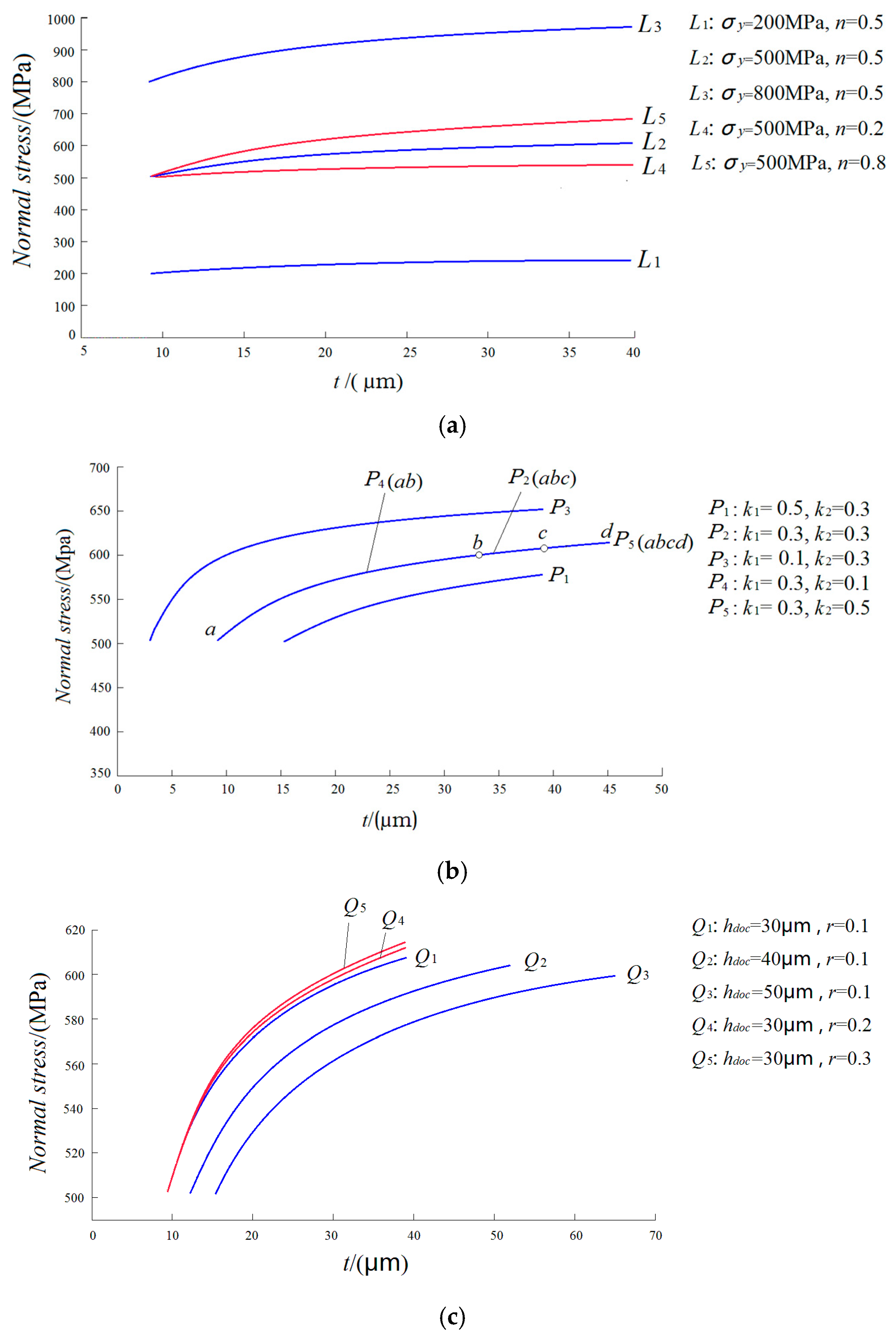
3.1. Normal Stress Distribution

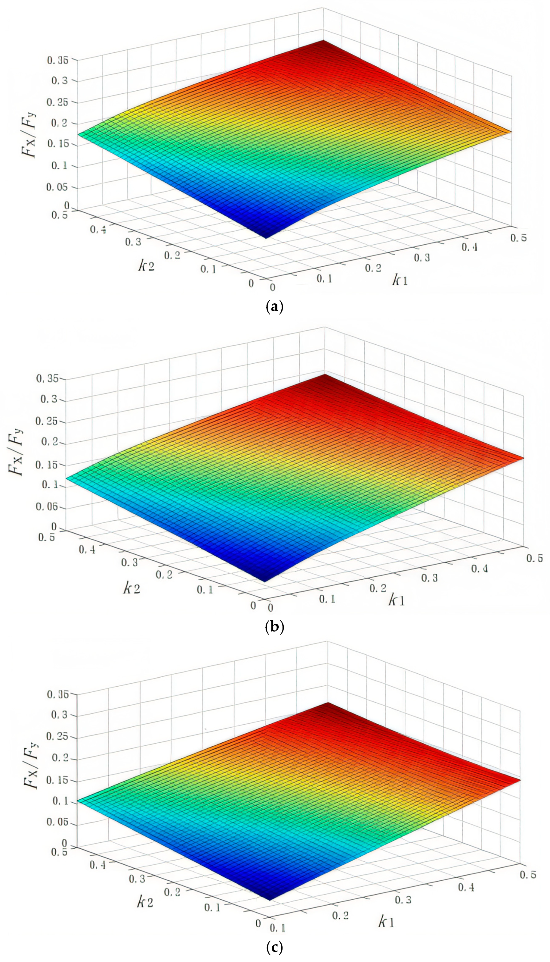
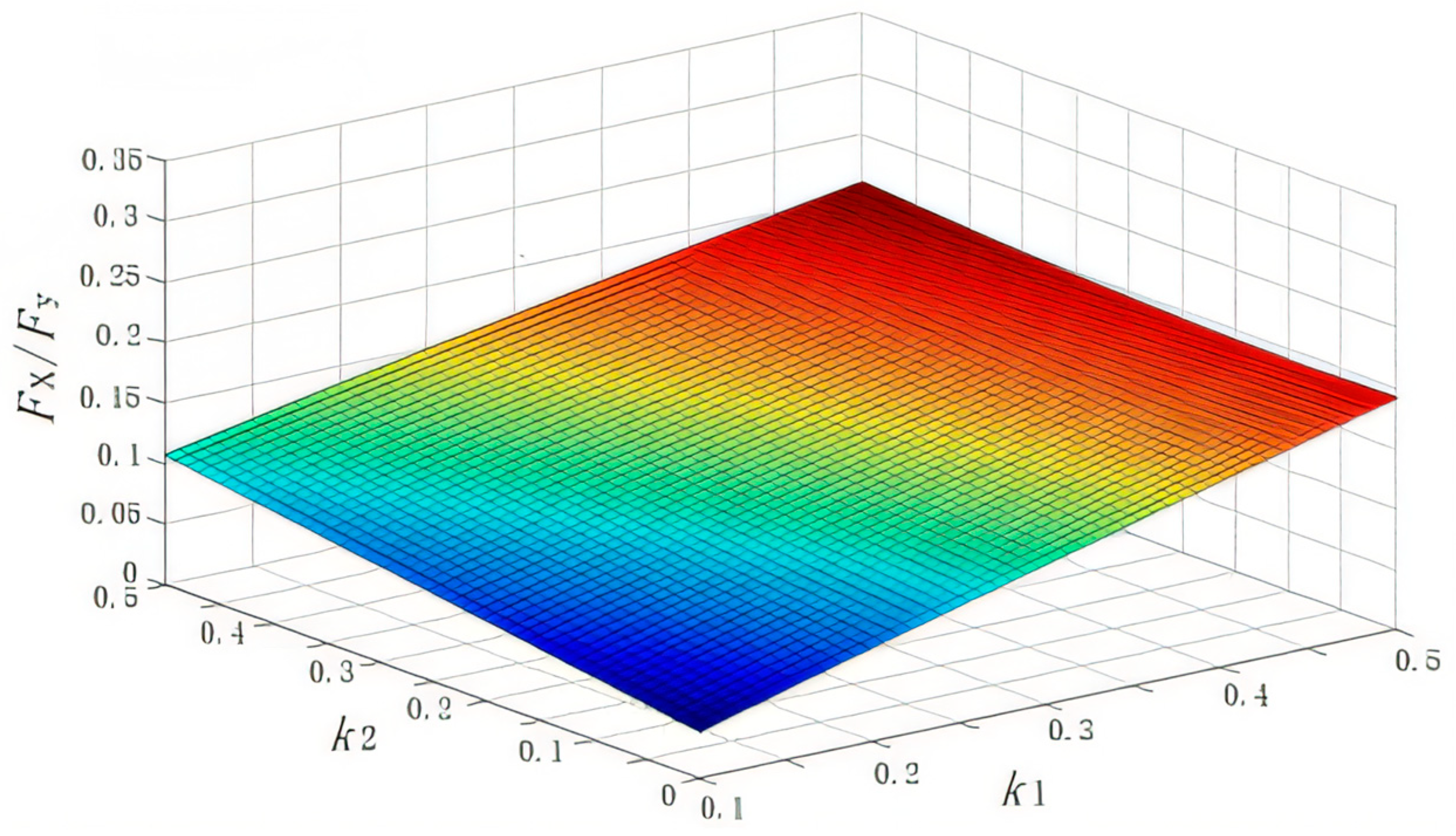
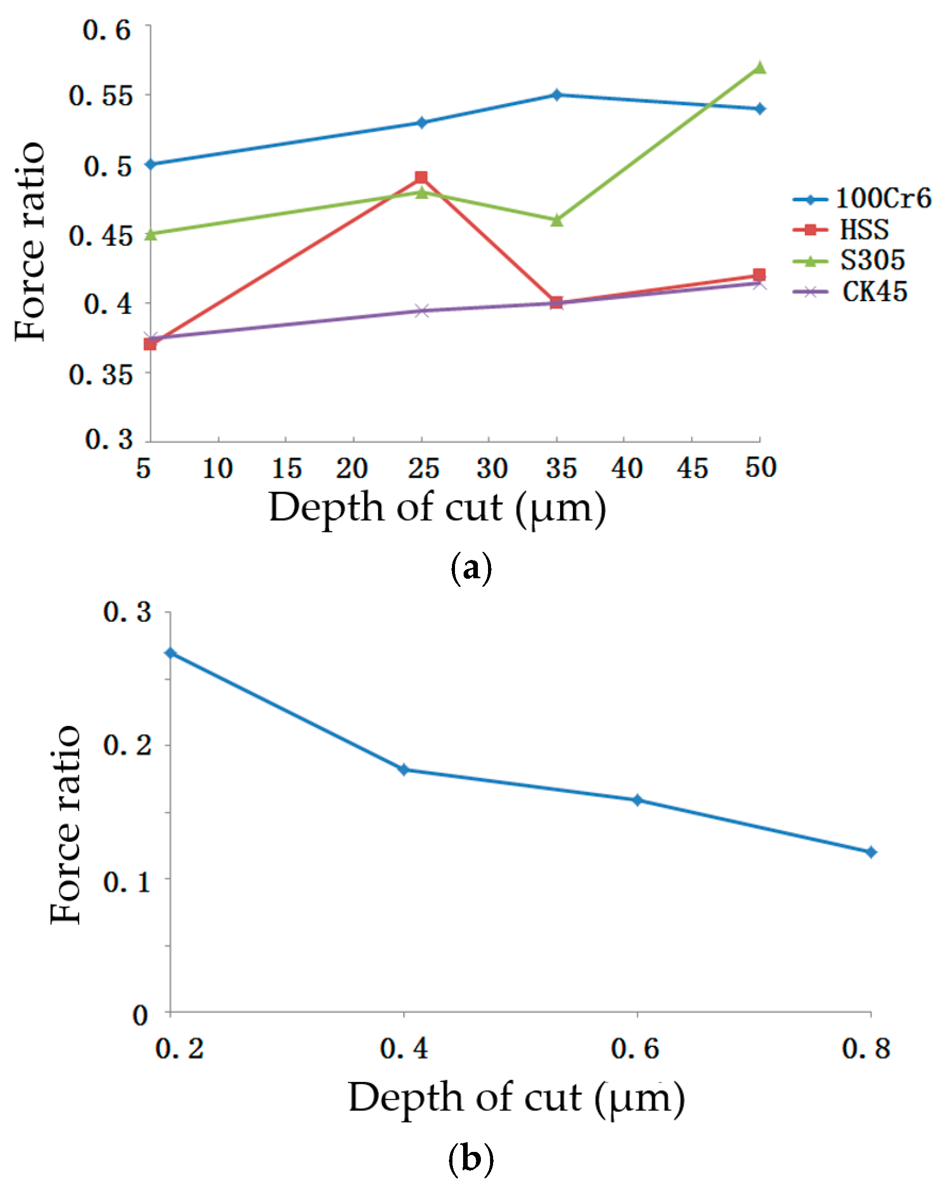
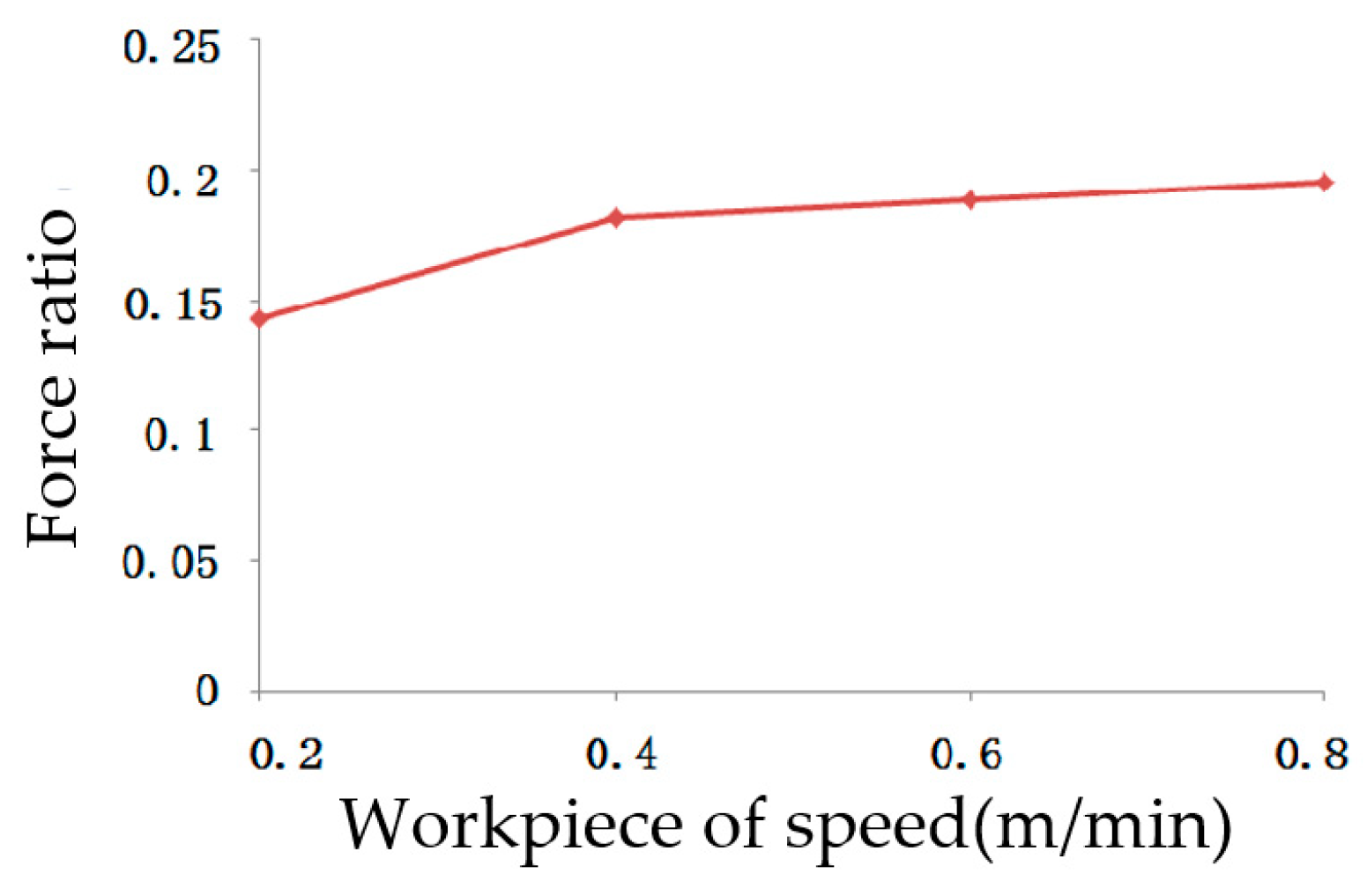
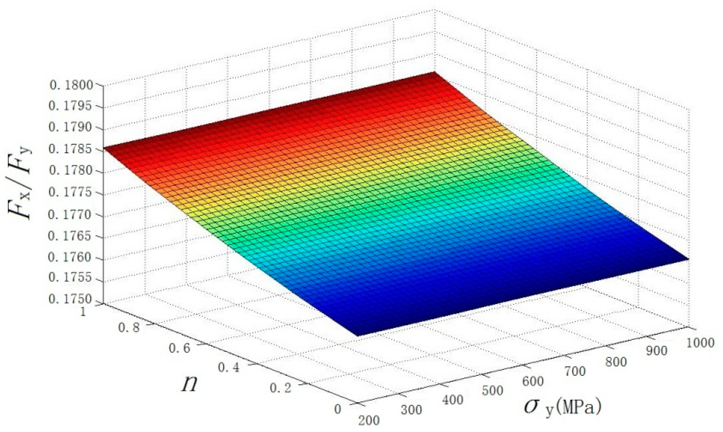
Normal stress distribution of the contact zone between the particle and workpiece can be obtained based on the analytical model when all parameters are determined, including nominal depth of cut h_doc, coefficient of elastic rebounds k₁, coefficient of plastic upheaval k₂, radius of particle r, yield strength σ_y, and coefficient of strain strengthening n of the material. Shear stress distribution will be obtained based on normal stress distribution and considering the coefficient of friction. The normal stress distribution on the elastic deformation zone conforms to the Hertz contact theory, which is common, and Equation (7) provides a clear indication. The normal stress on the plastic deformation zone can be calculated according to Equations (16) and (17). All parameters have been considered to draw a series of normal stress distribution curves in the plastic deformation zone, which also express the effect of these parameters on normal stress distribution. All curves have been classified, and the parameters for each specific curve are listed in

Table 1. Parameters of normal stress distribution curves on plastic deformation zone.

Curves	σy/MPa	N	hdoc/μm	r/mm	k1	k2
L1	200	0.5	30	0.1	0.3	0.3
L2	500	0.5	30	0.1	0.3	0.3
L3	800	0.5	30	0.1	0.3	0.3
L4	500	0.2	30	0.1	0.3	0.3
L5	500	0.8	30	0.1	0.3	0.3
P1	500	0.5	30	0.1	0.1	0.3
P1	500	0.5	30	0.1	0.3	0.3
P1	500	0.5	30	0.1	0.5	0.3
P1	500	0.5	30	0.1	0.3	0.1
P1	500	0.5	30	0.1	0.3	0.5
Q1	500	0.5	30	0.1	0.3	0.3
Q2	500	0.5	40	0.1	0.3	0.3
Q3	500	0.5	50	0.1	0.3	0.3
Q4	500	0.5	30	0.2	0.3	0.3
Q5	500	0.5	30	0.3	0.3	0.3

.

The curves were drawn in three coordinate systems according to the classification of Table 1. The results are shown in Figure 4.

As shown in Figure 4, the normal stress increases with the increase in t in the plastic deformation zone, and the rate of increase decreases gradually. The maximum normal stress appears at the separation point of the chip and the particle, as well as the shear stress. Therefore, the wear degree of separation point is the largest. As shown in Figure 4a, the normal stress increases with the increase in yield strength σ_y and the coefficient of strain strengthening n. The greater yield stress, the greater normal stress under the same deformation levels, and the greater strain strengthening, the greater the growth rate of normal stress with the increase in strain, which leads to the phenomenon shown in Figure 4a.

As shown in Figure 4b, the normal stress increases with the increase in rebound height h₁, and at the starting point of curves P₁(k₁ = 0.5), P₂ (k₁ = 0.3), and P₃(k₁ = 0.1), the values of normal stress are equal. At the end of the curves, the value decreases with the increase in the coefficient of elastic rebound k₁; for example, the normal stress decreases from 650.6 MPa to 577.8 MPa when the coefficient of elastic rebound k₁ increases from 0.1 to 0.5. The reason is that the increase in elastic rebound leads to an increase in the origin length of plastic deformation defined in Section 2.1, in return, leading to a decrease in maximum strain. The change in coefficient of plastic upheaval k₂ just changes the length of normal stress distribution curves, and the value of the curves does not change; for example, curves P₄ (ab) and P₂ (abc) are included in curve P₅ (abcd), because the coefficient of plastic upheaval for curve P₅ is the biggest, so the vertical height of plastic deformation and the maximum strain are bigger than others. It is the reason that the greater the coefficient of plastic upheaval, the longer the normal stress distribution curve, and the greater the maximum normal stress.

As shown in Figure 4c, a smaller nominal depth of cut (h_doc) results in a higher maximum normal stress when both the coefficient of elastic rebound (k₁) and the coefficient of plastic upheaval (k₂) remain constant. For example, the normal stress of the end of curve Q₁ (h_doc = 30 μm) is 607.6 MPa, the end of curve Q₂ (h_doc = 40 μm) is 603.9 MPa, and the end of curve Q₃ (h_doc = 50 μm) is 599.5 MPa. Both the origin length of plastic deformation and the maximum length of plastic deformation increase as the increase in nominal depth of cut h_doc due to the coefficient of elastic rebounds k₁ is constant, but the origin length of plastic deformation has a greater rate which results in the strain decreasing with the increase in h_doc. The bigger the particle radius r, the bigger the maximum normal stress.

3.2. Force Ratio

The forces applied to the particle are affected by three types of parameters, which may impact on force ratio. One kind is related to dimensions including k₁, k₂, r, and h_doc. Another kind is associated with the material constitutive model (yield strength σ_y and coefficient of strain strengthening n). The last one is the coefficient of friction μ. In order to study the effect of these parameters on force ratio, a MATLAB R2021b program was made according to the analytical model as shown in the appendix to calculate the forces applied on the particle directly, then the force ratio can be obtained.

The coefficient of elastic rebound k₁ and the coefficient of plastic upheaval k₂ represent the relative height of elastic rebound and plastic upheaval, respectively. The friction coefficient μ expresses the linear relationship between the normal stress and shear stress, which is common sense, and may influence the force ratio. In the scratching process, the force ratio depends on k₁, k₂, and μ when other parameters are given. A series of experiments were conducted to research how k₁, k₂, and μ affect the force ratio. The experimental setup is listed in

Table 2. Experimental setup for studying the effect of k₁, k₂, and μ.

	σy = 500 MPa, hdoc = 30 μm, n = 0.5, r = 0.1 mm
	μ = 0.3/0.4/0.5
	k11	k12	k13	k14	k15
k21	(0.1,0.1)	(0.1,0.2)	(0.1,0.3)	(0.1,0.4)	(0.1,0.5)
k22	(0.2,0.1)	(0.2,0.2)	(0.2,0.3)	(0.2,0.4)	(0.2,0.5)
k23	(0.3,0.1)	(0.3,0.2)	(0.3,0.3)	(0.3,0.4)	(0.3,0.5)
k24	(0.4,0.1)	(0.4,0.2)	(0.4,0.3)	(0.4,0.4)	(0.4,0.5)
k25	(0.5,0.1)	(0.5,0.2)	(0.5,0.3)	(0.5,0.4)	(0.5,0.5)

Remark: k_1i represents the value of k₁, k_2j represents the value of k₂, and (s, t) represents k_2j = s, k_1i = t.

, and the results are shown in Figure 5.

As shown in Figure 5, the force ratio increases almost linearly with the increase in the coefficient of elastic rebound k₁ and the coefficient of plastic upheaval k₂. As shown in Figure 5b, the force ratio increases from 0.1932 to 0.2453 as k₂ increases from 0.1 to 0.5 (k₁ = 0.3), an increase of 0.0521; the force ratio from 0.1769 to 0.2491 when k₁ from 0.1 to 0.5 (k₂ = 0.3), an increase of 0.0722. So, k₂ has more influence on the force ratio than k_1, which can also be seen from Figure 5 intuitively. The conclusion can also be drawn that the smaller the friction coefficient, the larger the force ratio. For example, assuming both k₁ and k₂ are 0.3, when μ is 0.4, 0.5, and 0.6, the corresponding force ratios are 0.2186, 0.1774, and 0.1403, respectively. However, previous studies have shown that the force ratio (F_t/F_n) increases with the increase in friction coefficient [18]. Some research has shown that the friction coefficient affects k₁ and k₂ [19], but this study assumes that μ, k_1, and k₂ were independent of each other because the relationships among them are too complex to reflect in the analytical model. This is the reason for the contradiction.

The force ratio depends on r and h_doc when other parameters are given. The experimental setup for researching the effect of r and h_doc on force ratio is listed in

Table 3. Experimental setup for studying the effect of h_doc and r.

	σy = 500 MPa, k1 = k2 =0.3, μ = 0.5, n = 0.5
	hdoc1	hdoc2	hdoc3	hdoc4	hdoc5
r1	(0.05,30)	(0.05,35)	(0.05,40)	(0.05,45)	(0.05,50)
r2	(0.10,30)	(0.10,35)	(0.10,40)	(0.10,45)	(0.10,50)
r3	(0.15,30)	(0.15,35)	(0.15,40)	(0.15,45)	(0.15,50)
r4	(0.20,30)	(0.20,35)	(0.20,40)	(0.20,45)	(0.20,50)
k5	(0.25,30)	(0.25,35)	(0.25,40)	(0.25,45)	(0.25,50)

Remark: h_doci represents the value of h_doc, r_j represents the value of r. (s, t) represents r_j =s, h_doci =t.

, and the result is shown in Figure 6.

As shown in Figure 6. It was found that the force ratio increases almost linearly with the increase in nominal depth of cut h_doc, and the increase rate is related to particle radius; the smaller the particle radius, the greater the increase in force ratio. For example, when the particle radius is 0.05 mm, h_doc from 30 mm to 50 mm, the force ratio increased by 0.3261, and when the particle radius is 0.20 mm, h_doc from 30 mm to 50 mm, the force ratio increased by 0.08286. It was also found that the force ratio decreases with the increase in particle radius, which agrees with the common sense that blunt abrasives are difficult to engage in the workpiece, and the force ratio decreases more rapidly with small particle radius. At the same time, the decrease is associated with the nominal depth of cut h_doc. For example, when the h_doc is 30 μm, r from 0.05 mm to 0.25 mm, the force ratio decreased by 0.3547, and when the h_doc is 50 μm, h_doc from 0.05 mm to 0.25 mm, the force ratio decreased by 0.6082. The force ratio variation trend is the change in particle radius and the nominal depth of cut.

The present study has shown that the force ratio increases with the increase in depth of cut. In the grinding process, grinding depth, workpiece speed, and grinding speed could lead to a change in single-particle cutting depth. Two soft steels (CK45 and S305) and two hard steels (HSS and 100Cr6) have been used for the grinding test; it was found that the force ratio almost increases with the increase in grinding depth when the grinding condition is dry, as shown in Figure 7a. At the same time, when the grinding condition is MQL or conventional fluid, the force ratio has the same variation [20]. Some studies have shown that the force ratio decreases as the grinding depth increases, as illustrated in Figure 7b [21]. Specifically, an increase in grinding depth not only leads to a greater single-particle cutting depth but also causes some previously non-engaged abrasive particles to start participating in the cutting process with shallow depths of cut. This observation does not conflict with the conclusions of this study.

The single-particle cutting depth increases with the increase in workpiece speed in the grinding process. The 65Mn workpiece dry grinding tests were carried out, the grinding test results showed in Figure 8 that the force ratio increases with the increase in workpiece speed [21]. A series of grinding experiments were conducted, and it was found that the force ratio (F_t/F_n) almost increases with the workpiece increasing [22]. The single-particle cutting depth decreases with the increase in grinding speed in the grinding process. A vitreous bond cBN wheel grinding experiment has been implemented, and it was found that the force ratio (F_t/F_n) decreases with the increase in grinding speed for both the Zirconia and M₂ steel workpieces [23].

The present study showed that the force ratio decreases with the increase in grit size [24]; the result is shown in Figure 9. This result is consistent with the conclusion of this study.

The material constitutive model includes two parameters that yield strength σ_y and the coefficient of strain strengthening n. The force ratio depends on σ_y and n when other parameters are given. The experimental setup for researching the effect of σ_y and n on force ratio is listed in

Table 4. Experimental setup for studying the effect of material constitutive model.

	hdoc = 30 μm, k1 = k2 = 0.3, μ = 0.5, r = 0.1 mm
	σy1	σy2	σy3	σy4	σy5
n1	(0.2,200)	(0.2,400)	(0.2,600)	(0.2,800)	(0.2,1000)
n2	(0.4,200)	(0.4,400)	(0.4,600)	(0.4,800)	(0.4,1000)
n3	(0.6,200)	(0.6,400)	(0.6,600)	(0.6,800)	(0.6,1000)
n4	(0.8,200)	(0.8,400)	(0.8,600)	(0.8,800)	(0.8,1000)
n5	(1,200)	(1,400)	(1,600)	(1,800)	(1,1000)

Remark: σ_yi represents the value of σ_y, n_j represents the value of n. (s, t) represents n_j = s, σ_yi = t.

, and the result is shown in Figure 10.

As shown in Figure 10, the force ratio affected by the material constitutive model was presented. A conclusion can be drawn that σ_y does not affect the force ratio. The force ratio increases linearly with the increase in n, but the increase is not obvious. The reason is that both the elastic deformation zone and the plastic deformation zone are involved in the parameter σ_y, but only the plastic deformation zone is involved in the parameter n. During the elastic contact phase, the smaller contact area leads to local stress concentrations that may promote material cutting rather than furrow formation, resulting in a higher plough–cut ratio (i.e., a higher percentage of cutting). Plastic deformation leads to redistribution of the contact area. It has been shown that the ratio of plastic contact area to plastic contact area decreases significantly during wear, especially when the ratio is below 0.5, and wear increases dramatically, suggesting that the material is removed in the form of flaking rather than sustained plough-cutting. In addition, the work hardening of elasto-plastic materials enhances resistance to plastic deformation, further reducing the plastic contact area and leading to a decrease in wear [25]. This dynamic change may cause the force ratio to decrease as the plastic phase progresses.

The energy dissipation mainly originates from the hysteresis effect of viscoelastic materials and the deformation of the adhesion neck at the contact edge. Under elastic conditions, increased adhesion strength may lead to increased friction, but the energy release rate shows a non-monotonic trend [26]. At this time, energy accumulation is dominated by microconvex body deformation, with less material removal and potentially higher force ratios. Plastic deformation dominates energy dissipation. During friction, the subsurface maximum shear stress triggers fatigue crack initiation and extension, leading to material stripping to form abrasive debris, and energy is released through plastic deformation and thermal dissipation (frictional temperature rise). For example, frictional temperature rise can cause plastic deformation of the contact surface to expand and significantly increase wear [27]. The energy dissipation in the plastic phase is more focused on material destruction rather than furrow formation and may reduce the force ratio.

The elastic contact stresses are not uniformly distributed, with peak stresses occurring at the contact edges (e.g., the leading edge of slider motion), which tends to initiate surface/subsurface cracking in brittle materials [28,29]. At this time, the stress concentration promotes cutting action and improves the force ratio. For example, hard and brittle materials are susceptible to crack extension paths predicted by the principal stress-to-hardness ratio model in an elastic stress field [28]. The plastic contact stress distribution tends to be uniform, but the subsurface stress distribution is closely related to the microstructural evolution. Molecular dynamics simulations show that when the stress in the plastic phase of single-crystal nickel exceeds a threshold value, the internal plastic ring sheds to release the stress, leading to the removal of the material in the form of plastic flow [30]. In addition, in the elasto-plastic model, the tangential force increases while slip decreases as the contact half-width increases, and the frictional dissipation energy decreases, which may reduce the cutting action [31]. Uniform stress distribution is more likely to form furrows rather than cutting, reducing the force ratio.

4. Conclusions

The physical and analytical models of the scratching process have been presented. The workpiece material deformation during the scratching process has been divided into the elastic and plastic deformation zones, and the mechanical expression of cutting forces in the elastic and plastic deformation zones has been presented, respectively.

The coefficient of elastic rebounds k₁ and the coefficient of plastic upheaval k₂ have been defined to describe the degree of elastic rebounds back and plastic upheaval, respectively.

The stress distribution on the plastic deformation zone according to the analytical model has also been given and was studied further.

This study systematically analyzed all parameters influencing the force ratio, conducting simulation experiments using MATLAB. Simulation results were quantitatively analyzed, and the model’s validity was further corroborated by referencing findings from published literature. Key observations include: the force ratio increases with an increase in the elastic rebound coefficient, plastic upheaval coefficient, nominal cut depth, and strain-strengthening coefficient, but decreases as particle radius grows. Notably, the nominal cut depth may underestimate the actual indentation depth due to elastic rebound, directly impacting material removal efficiency. A higher k₁ (elastic rebound coefficient) amplifies elastic recovery, reducing the effective cut depth; a higher k₂ (plastic upheaval coefficient) enhances material bulging along scratch edges, potentially degrading surface quality. Balancing machining efficiency (favored by higher nominal depths) and surface quality (favored by lower nominal depths) can be achieved through strategic adjustment of nominal cut depth. The strain-to-force ratio, which links force–displacement curves during plastic deformation, serves as a critical parameter for modeling cutting forces. Importantly, yield stress was found to have no discernible effect on the force ratio, distinguishing it from other analyzed parameters. Finally, although this paper proposes a physical model and an analytical model of a single abrasive grain in the grinding process, this paper makes relevant assumptions and simplifications to the relevant models; for example, this paper assumes the irregular geometry of the abrasive grain as a perfect sphere for the relevant research, which may lead to result in the insufficient adaptability of the model to complex working conditions. This paper also simplifies the sliding friction process to Hertzian contact and homogenises the material, and these simplifications can limit the applicability of the model in extreme conditions. In addition, the model proposed in this paper does not consider the relevant situation of high temperature and high speed.

In the future, scholars can consider the actual shape of the particles for related research, and the analysis of the slipping and rubbing process of multilayer structural materials is also one of the future research directions; in addition, a thermally coupled high temperature and high-speed model can be established to study the behaviour of abrasive particles under high temperature and high-speed conditions.

References

1. Barge, M.; Rech, J.; Hamdi, H.; Bergheau, J. Experimental study of abrasive process. Wear 2008, 264, 382–388. [Google Scholar] [CrossRef]
2. Singh, V.; Venkateswara Rao, P.; Ghosh, S. Development of specific grinding energy model. Int. J. Mach. Tools Manuf. 2012, 60, 1–13. [Google Scholar] [CrossRef]
3. Pandiyan, V.; Caesarendra, W.; Tjahjowidodo, T.; Praveen, G. Predictive modelling and analysis of process parameters on material removal characteristics in abrasive belt grinding process. Appl. Sci. 2017, 7, 363. [Google Scholar] [CrossRef]
4. Wang, Y.; Chen, Y.; Qi, F.; Xing, Z.; Liu, W. A molecular-scale analytic model to evaluate material removal rate in chemical mechanical planarization considering the abrasive shape. Microelectron. Eng. 2015, 134, 54–59. [Google Scholar] [CrossRef]
5. Awan, M.R.; Rojas, H.A.G.; Benavides, J.I.P.; Hameed, S.; Hussain, A.; Egea, A.J.S. Specific energy modeling of abrasive cut off operation based on sliding, plowing, and cutting. J. Mater. Res. Technol. 2022, 18, 3302–3310. [Google Scholar] [CrossRef]
6. Shaik, J.H.; Srinivas, J. Analytical prediction of chatter stability of end milling process using three-dimensional cutting force model. J. Braz. Soc. Mech. Sci. Eng. 2017, 39, 1633–1646. [Google Scholar] [CrossRef]
7. Chang, H.; Wang, J.J.J. A stochastic grinding force model considering random grit distribution. Int. J. Mach. Tools Manuf. 2008, 48, 1335–1344. [Google Scholar] [CrossRef]
8. Da Silva, W.M.; de Mello, J.D.B. Using parallel scratches to simulate abrasive wear. Wear 2009, 267, 1987–1997. [Google Scholar] [CrossRef]
9. Sinha, S.K.; Chong, W.L.M.; Lim, S. Scratching of polymers—Modeling abrasive wear. Wear 2007, 262, 1038–1047. [Google Scholar] [CrossRef]
10. Zhang, F.; Meng, B.; Geng, Y.; Zhang, Y. Study on the machined depth when nanoscratching on 6H-SiC using Berkovich indenter: Modelling and experimental study. Appl. Surf. Sci. 2016, 368, 449–455. [Google Scholar] [CrossRef]
11. Horng, T. Modeling and simulation of material removal in planarization process. Int. J. Adv. Manuf. Technol. 2008, 37, 323–334. [Google Scholar] [CrossRef]
12. Chen, X.; Zhao, Y.; Wang, Y. Modeling the effects of particle deformation in chemical mechanical polishing. Appl. Surf. Sci. 2012, 258, 8469–8474. [Google Scholar] [CrossRef]
13. Torrance, A.A. Modelling abrasive wear. Wear 2005, 258, 281–293. [Google Scholar] [CrossRef]
14. Jourani, A.; Dursapt, M.; Hamdi, H.; Rech, J.; Zahouani, H. Effect of the belt grinding on the surface texture: Modeling of the contact and abrasive wear. Wear 2005, 259, 1137–1143. [Google Scholar] [CrossRef]
15. Baranowski, P.; Damaziak, K.; Malachowski, J.; Sergienko, V.P.; Bukharov, S.N. Modeling of abrasive wear by the meshless smoothed particle hydrodynamics method. J. Frict. Wear 2016, 37, 94–99. [Google Scholar] [CrossRef]
16. Miyoshi, K. Solid Lubrication Fundamentals and Applications, 1st ed.; CRC Press: Boca Raton, FL, USA, 2001; pp. 1–4. [Google Scholar]
17. Jiang, F.; Yan, L.; Rong, Y. Orthogonal cutting of hardened AISI D2 steel with TiAlN-coated inserts—Simulations and experiments. Int. J. Adv. Manuf. Technol. 2013, 64, 1555–1563. [Google Scholar] [CrossRef]
18. Sanchez, J.A.; Pombo, I.; Alberdi, R.; Izquierdo, B.; Ortega, N.; Plaza, S.; Martinez-Toledano, J. Machining evaluation of a hybrid MQL-CO2 grinding technology. J. Clean. Prod. 2010, 18, 1840–1849. [Google Scholar] [CrossRef]
19. Chen, X.; Tecelli Öpöz, T. Simulation of Grinding Surface Creation—A Single Grit Approach. Adv. Mater. Res. 2010, 126–128, 23–28. [Google Scholar] [CrossRef]
20. Rabiei, F.; Rahimi, A.R.; Hadad, M.J.; Ashrafijou, M. Performance improvement of minimum quantity lubrication (MQL) technique in surface grinding by modeling and optimization. J. Clean. Prod. 2015, 86, 447–460. [Google Scholar] [CrossRef]
21. Liu, J.; Xiong, J.; Yuan, W. Experiment Study on Grinding Force of 65Mn Steel in Grinding-Hardening Machining; Springer: Berlin/Heidelberg, Germany, 2012; pp. 239–246. [Google Scholar]
22. Ding, W.; Zhao, B.; Xu, J.; Yang, C.; Fu, Y.; Su, H. Grinding behavior and surface appearance of (TiCp+TiBw)/Ti-6Al-4V titanium matrix composites. Chin. J. Aeronaut. 2014, 27, 1334–1342. [Google Scholar] [CrossRef]
23. Thammasing, V.; Tangjitsitcharoen, S. In-Process Prediction of Surface Roughness in Grinding Process by Monitoring of Cutting Force Ratio. Appl. Mech. Mater. 2014, 627, 29–34. [Google Scholar] [CrossRef]
24. Amamou, R.; Ben Fredj, N.; Fnaiech, F. Improved method for grinding force prediction based on neural network. Int. J. Adv. Manuf. Technol. 2008, 39, 656–668. [Google Scholar] [CrossRef]
25. Dang, X.; Huang, J.; Chen, S. Influence of Plastic Contact Area on Sliding Wear of GCr15/35CrMo Steel Tribo-pair. J. Tribol. 2015, 35, 8–14. [Google Scholar]
26. Persson, B.N.J.; Xu, R.; Miyashita, N. Rubber wear: Experiment and theory. J. Chem. Phys. 2025, 162, 074704. [Google Scholar] [CrossRef] [PubMed]
27. Tan, S.; Liu, J.; Shen, H.; Chen, Y. Numerical analysis of torsional micro-motion thermal coupling considering frictional heat generation. J. Chongqing Univ. Technol. (Nat. Sci.) 2022, 36, 119–125. [Google Scholar]
28. Qian, H.; Chen, M.; Qi, Z.; Teng, Q.; Qi, H.; Zhang, L.; Shan, X. Review on research and development of abrasive scratching of hard brittle materials and its underlying mechanisms. Crystals 2023, 13, 428. [Google Scholar] [CrossRef]
29. Huang, W.; Li, W.; Mao, F.; Huang, P. Distribution of force and wear analysis of surface contact. J. South China Univ. Technol. (Nat. Sci. Ed.) 2020, 48, 91–101. [Google Scholar]
30. Chen, J.; Qiu, X.; Li, K.; Yuan, J.; Zhou, D.; Liu, Y. Microstructure Evolution and Plastic Removal for Single Crystal Nickel Induced by Particle Scratching: Atomic Simulation Method. Chin. J. Mater. Res. 2022, 36, 511–518. [Google Scholar]
31. Li, L.; Xue, Y.; Miao, D.; Ruan, X.; Li, L.; Xie, M. Fretting wear behavior considering the contact of third body particles. J. Aerosp. Power 2025, 40, 296–306. [Google Scholar]
Figure 1. Physical schematic of the scratching process. (a) The particle scratching physical process (Scanning Electron Microscopy (SEM)) [16]. (b) Physical model of the scratching process.
Applsci 15 05670 g001
Figure 2. Physical model of scratching process. (a) Side view. (b) Top view.
Applsci 15 05670 g002
Figure 3. Analytical model two-body abrasive wear. (a) Side view. (b) Top view.
Applsci 15 05670 g003
Figure 4. Effect of parameters on normal stress distribution on plastic deformation zone. (a) Effect of material constitutive model on normal stress distribution (hdoc = 30 μm, r = 0.1 mm, k1 = k2 = 0.3). (b) Effect of k1 and k2 on normal stress distribution (σy = 500 MPa, n = 0.5, hdoc = 30 μm, r = 0.1 mm). (c) Effect of hdoc and r on normal stress distribution (σy = 500 MPa, n = 0.5, k1 = k2 = 0.3).
Applsci 15 05670 g004
Figure 5. Effect of k1 and k2 on force ratio (σy = 500 MPa, hdoc = 30 μm, n = 0.5, r = 0.1 mm): (a) μ = 0.4, (b) μ = 0.5, and (c) μ = 0.6.
Applsci 15 05670 g005
Figure 6. Effect of r and hdoc on force ratio (σy = 500 MPa, k1 = k2 = 0.3, μ = 0.5, n = 0.5).
Applsci 15 05670 g006
Figure 7. Effect of grinding depth on force ratio: (a) the grinding condition is dry, (b) the grinding condition is MQL or conventional fluid.
Applsci 15 05670 g007
Figure 8. Effect of workpiece speed on force ratio.
Applsci 15 05670 g008
Figure 9. Effect of grit size on force ratio.
Applsci 15 05670 g009
Figure 10. Effect of n and σy on force ratio (hdoc = 30 μm, k1 = k2 = 0.3, μ = 0.5, r = 0.1 mm).
Applsci 15 05670 g010