Optical Coherence Tomography-Based Fingerprint Presentation Attack Detection via Multi-Tissue Features Contribution Analysis

Abstract

Currently, unsupervised anti-spoofing methods suffer from low accuracy and susceptibility to irrelevant factors. In order to solve these problems, this paper analyzes the contribution of different fingertip tissue structures to anti-spoofing tasks and proposes an unsupervised anti-spoofing method based on the weighted contribution of tissue structures. Unsupervised OCT anti-spoofing methods suffer from weak robustness and lack comprehensive exploration of sub-dermal structure features. The proposed method introduces quantified weights of fingertip tissue contributions with self-attention through the Shapley value. The module can amplify crucial fingertip features and extracts more key fingertip information, thereby improving the anti-spoofing performance.

1. Introduction

Fingerprints, as one of the most common physiological features of the human body, are widely used in determining individual identity information [1]. With the development of technology, fingerprint recognition technology has been applied in various fields such as fingerprint payment, fingerprint unlocking, and Internet of Things applications [2,3,4]. However, the collection process of epidermis fingerprints is easily affected by the external environment, and it is difficult to ensure the imaging quality of epidermis fingerprints, which leads to a decrease in the accuracy of fingerprint recognition [5]. In addition, epidermis fingerprint traces can easily be replicated and the cost of forgery is low.

The emergence of 3D fingerprint collection technology can alleviate the impacts brought by the above problems. Finger skin is a layered tissue, which is divided into the stratum corneum, the epidermis layer, and the dermis layer; at the junction of the dermis and the epidermis, there exists a papillary layer [6], which is the source of the fingerprint structure. In the epidermis layer, there are spiral ducts that connect the sweat glands in the dermis to the sweat pores on the surface [7]. Therefore, sub-dermal fingerprints have strong resistance to deformation and damage, and can make up for defects in the imaging quality of epidermis fingerprints. Meanwhile, by jointly considering complex features such as sweat glands and the layered structure of finger skin, the difficulty of forging samples can be greatly increased.

Optical coherence tomography (OCT) technology [7] can achieve collection of the three-dimensional structure of the finger. It can not only detect the epidermis fingerprints on the finger but also detect the micron-level complex structures of multiple tissue layers within the skin. The 3D fingerprint dataset obtained through OCT technology provides a solid data foundation for the development of more efficient and accurate fingerprint anti-spoofing methods.

Due to the diversity of materials used to make spoof samples, anti-spoofing methods use zero-shot [8] or one-class sample [9,10,11] approaches to construct deep autoencoders. Only training on bona fide fingerprints can prevent attacks from unknown spoof materials.

Currently, OCT fingerprint anti-spoofing methods can be divided into feature-based and learning-based methods. In the early days, for bona fide and spoof samples, the method of manually annotating image features was usually chosen for anti-spoofing tasks. The annotated features include sweat pores [12], physiological features [13], etc. Bossen et al. [7] carried out anti-spoofing by judging the presence or absence of the papillary layer. Liu et al. [14] used sweat gland annotations to distinguish spoof samples. Gutierrez et al. [15] used the difference in the deformation amount between internal and external fingerprints to mark bona fide fingerprints. Ding et al. [16] proposed an anti-spoofing method based on one-class support vector machines. Darlow et al. first proposed a fully automatic detection method based on highly separable double-layer features, which detected spoof fingerprints with 100% accuracy [17]. The above methods are based on manual feature selection, meaning they require a large amount of work and are inefficient when dealing with large-scale datasets.

Learning-based methods can automatically extract the features of input samples, significantly improving the efficiency and generalization ability of anti-spoofing methods. They are mainly divided into two categories: supervised and unsupervised learning. Supervised learning methods learn relevant features through the labels of bona fide and spoof samples for judgment. Chugh et al. [6] cut OCT images into image patches and input them into a convolutional binary classification network for in-depth detection to judge the authenticity of samples. Nogueira et al. [18] verified the superiority of CNN in supervised fingerprint anti-spoofing methods. Sun et al. [19] proposed the ISAPAD dual-branch network to detect spoof samples by learning the internal structure and overall features of fingerprints. However, in the existing methods, the samples used for training and testing come from the same data domain, and the detection performance for spoof samples with unknown data distributions remains unknown. It can be seen that these supervised methods rely on the limited attack samples in the training set and still have the problem of insufficient generalization ability when facing unknown attack samples. In contrast, in view of the diversity and unknown nature of spoof samples, unsupervised methods that only train on bona fide samples are more valuable in practical applications. Liu et al. [9] proposed an autoencoder method based on activation map reconstruction. Without any spoof samples for reference, it not only has better generalization ability but also alleviates the data dependence problem caused by the significant differences between different spoof samples. This method can achieve a true positive rate of 96.59% without using spoof fingerprints. Zhang et al. [20] found that there is noise interference in OCT scanned images. Therefore, by extracting the frequency information in the OCT spatio-temporal domain, decomposing the images into four different groups of frequency-domain information, and using wavelet decomposition to remove irrelevant interference information, they improved the performance by 81.89%. Liu et al. [21] introduced a prototype reconstruction module into the denoising autoencoder, used the sparse addressing method to find the prototype most similar to the input image in the memory module, and proposed a representation consistency constraint to make the reconstructed features closer to bona fide fingerprints, thereby increasing the reconstruction distance of spoof samples and reducing the error rate by 40.07%. Zhang et al. [22] proposed a brand-new unified representation model. By introducing an anti-spoofing task during the fingerprint reconstruction process, the intermediate features are connected and interact across layers, enabling both the reconstruction task and the anti-spoofing method to achieve good performance.

However, through the study of attention heat maps, it can be found that for fingerprints, the key information for judging the authenticity of samples is often concentrated in specific areas of the fingerprints. Most existing methods are based on the overall image. Therefore, there is still an overfitting phenomenon in the anti-spoofing task, a large number of sample features need to be annotated, and the reconstruction distance based on images cannot distinguish between bona fide and spoof samples.

In view of the diversity and unknown nature of spoof materials, a more robust anti-spoofing method is needed to ensure the security of fingerprint recognition systems. In this paper, a self-built 1310 nm OCT system is used to collect three-dimensional structural information on fingertips, and an unsupervised fingerprint anti-spoofing method that only requires bona fide samples is proposed, which can more accurately judge the authenticity of samples. Subsequently, a CNN is used to conduct ablation comparison experiments on different sub-dermal tissue structures of the fingers, and the contribution of these structures in the fingerprint anti-spoofing task is analyzed, providing strong evidence for the method proposed in this paper. The specific research contents are as follows:

In order to further analyze the importance of different tissue structures of bona fide samples for the anti-spoofing task, starting from the characteristics of multiple local features and overall features of OCT fingerprints that can be used for anti-spoofing, this paper explores the correlation between the internal features of fingerprints and their contribution to the anti-spoofing task, and improves the performance of the anti-spoofing method by formulating relevant analysis criteria. Through the correlation study of all local 3D features and relevant anti-spoofing tasks, the degree of dependence of each task on fingerprint features is quantitatively analyzed. The model training process not only relies on a single 3D feature of bona fide samples but also comprehensively considers the relationships among the overall features, local features, and anti-spoofing tasks, so as to improve the anti-spoofing performance of the model. Finally, based on the visualization segmentation results of bona fide samples and spoof samples, starting from the data distribution of the input samples, the spoof score criteria are established by using the mean and variance of the Gaussian distribution of features, which are used for the detection of spoof samples.

The remainder of this article is organized as follows. In Section 2, we review some related work about OCT technology and deep learning visual model architectures. We introduce our proposed unsupervised anti-spoofing method in Section 3. Section 4 shows related experimental results and compares the performance of our method with other unsupervised models. In Section 5, we summarize the research methods of this paper, describe deficiencies and improvement directions related to the current research, and explain the next steps pertaining to our work.

2. Related Work

This section first introduces the OCT collection system and related technologies adopted in the experiment. Subsequently, it describes the characteristics of OCT images of bona fide samples and those of spoof samples, and provides an overview of the existing OCT fingerprint anti-spoofing methods and their performance evaluation metrics. Finally, it describes the deep learning theory involved in the method proposed in this paper.

2.1. OCT Fingerprint Collection Device System

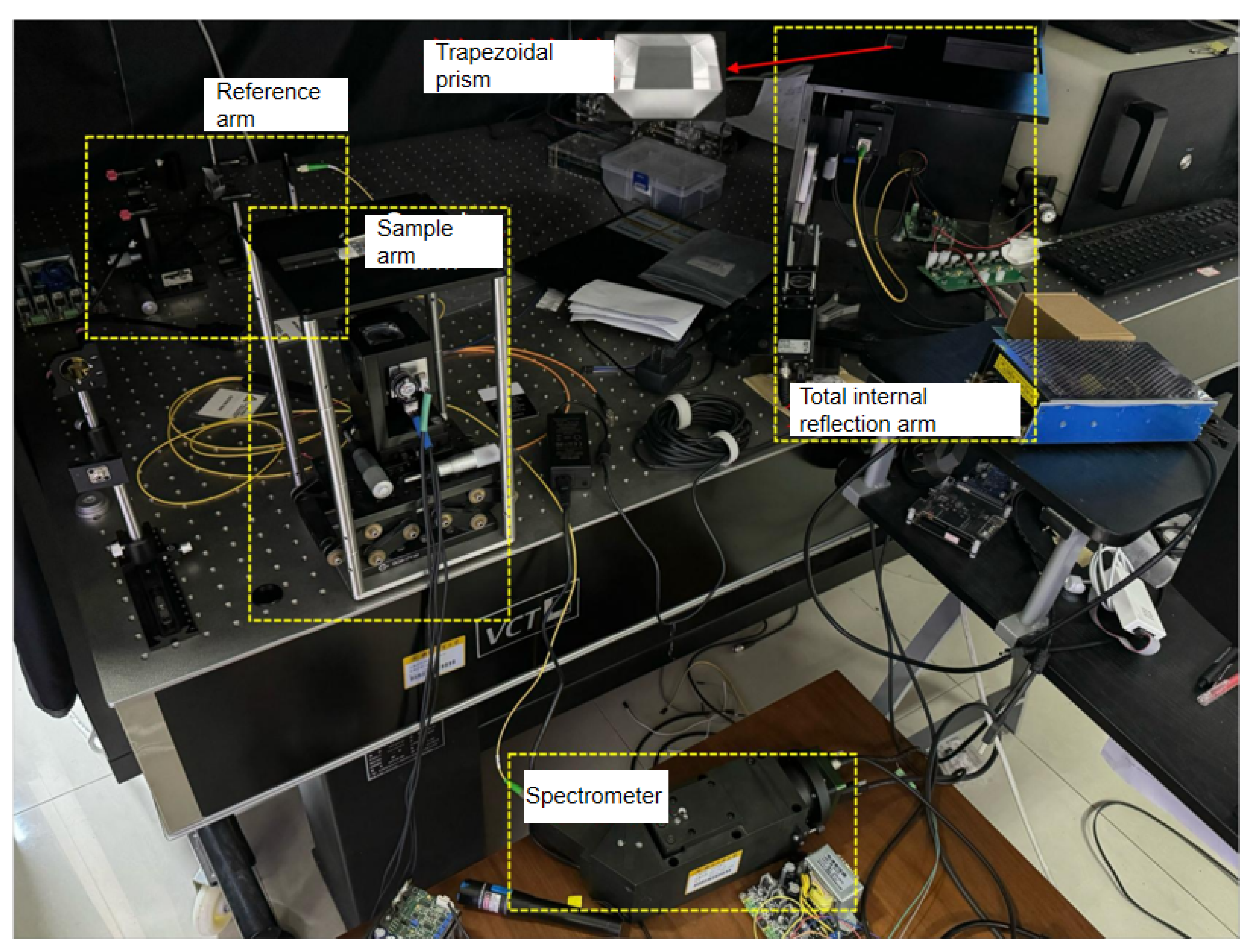
OCT technology can achieve high-resolution acquisition of three-dimensional volume data of fingertips. This technology utilizes the principle of low-coherence interference of near-infrared light (780 nm–2526 nm). By measuring the optical reflection of internal tissues, it realizes non-invasive and high-resolution cross-sectional imaging and has been widely applied in the biomedical field [7]. As shown in Figure 1, in an OCT scanner, the light beam is divided into a reference arm and a sample arm, each containing a mirror unit. If the reflected light from the two arms is within the coherence distance, an interference pattern will be generated. This interference pattern represents the depth profile at a point, which is called an A-scan. A 2D image at a fixed depth is called an enface slice; laterally combining a series of A-scans along a line can provide a cross-sectional pattern, which is called a B-scan image; stacking multiple B-scan images together can represent the volume data structure of the scanned fingerprint. In the data acquisition stage, the finger must be placed tightly on a thin glass sheet and kept still to ensure the stability of the system during data collection.

Our laboratory has independently developed an OCT scanning system to collect the tissue information from fingertips, as shown in Figure 1. It uses a broadband source with a central wavelength of 1310 nm and a bandwidth of 85.6 nm. The light can penetrate through the stratum corneum and the epidermis layer until reaching the dermis layer, and the maximum scanning depth can reach 4.64 mm beneath the skin. Each collection of fingertip volume data contains 1400 or 700 B-scan images. The size of each B-scan image is 1800 × 500, as shown in Figure 2.

2.2. OCT Dataset

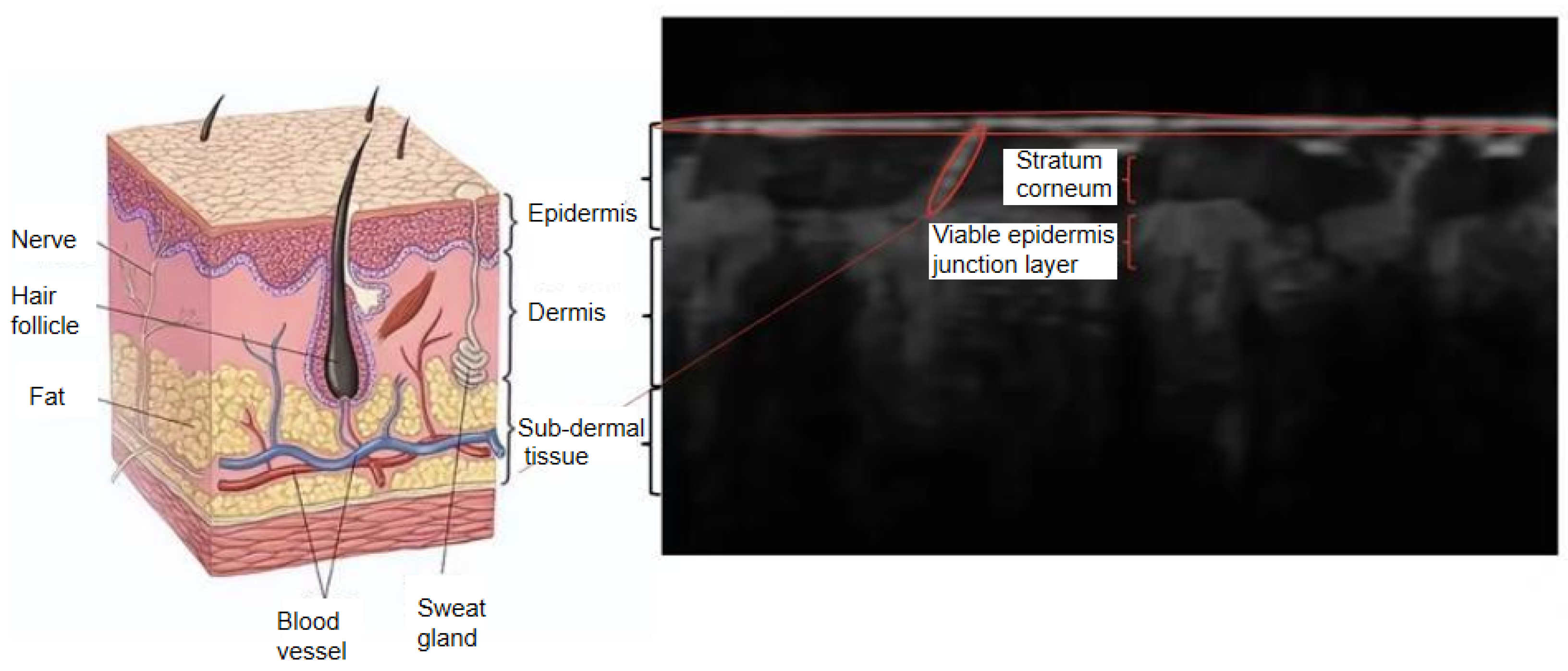
The corresponding relationship between the B-scan images acquired by OCT technology and the real sub-dermal structures of fingertips is shown in Figure 3. The outermost layer, which comes into daily contact with the external environment, is called the epidermis. On the outer surface of the epidermis, the tough part with friction ridge structures is known as the stratum corneum. The part beneath the epidermis is the dermis, which provides most of the skin’s elasticity and strength. Sweat glands are distributed between the epidermis and the dermis, usually in a spiral or oval shape, and are responsible for secreting sweat to regulate body temperature. The special structure located between the stratum corneum and the dermis is the viable epidermis junction layer. This layer has unique undulating features, called the internal fingerprint, which provides a basis for identifying an individual’s identity.

The bona fide samples used in the experiment were collected from 160 white-collar and blue-collar workers aged between 20 and 60, with a ratio of approximately 1:4. All the volunteers who participated in the fingerprint collection were Chinese. A total of 2,039,800 slices were collected. Due to the issue of the slicing angle during scanning, the first 400 B-scan slices of each volume of data do not have a relatively complete tissue structure. Therefore, in the experiment, only the last 1000 scanned slices of each volume of data were selected as the source of the bona fide sample dataset.

In this paper, 21 kinds of materials are used to make the spoof sample dataset, with a total of 525 groups of spoof sample data. The spoof sample dataset is roughly divided into two categories. The first category uses a single material, which can only ensure that the surface threads of the samples are similar to those of bona fide fingerprints. The materials used include epoxy resin, Elmer’s glue, handmade white glue, conductive silica gel, etc. The other category of spoof samples has a double-layer tissue structure similar to that of the OCT images of bona fide samples, which increases the difficulty of the anti-spoofing task. This type of spoof sample is composed of eight kinds of materials, including transparent silica gel, flesh-colored silica gel, etc.

As shown in

Table 1. Fake fingerprint example.

Fingerprint Example	Actual Image	OCT Scan Image
Bona fide fingerprint
Single-layer structure, flesh-colored silica gel
Single-layer structure, fingerprint film
Ultra-thin fingerprint film, transparent silica gel
Double-layer fingerprint film, flesh-colored silica gel
Double-layer ultra-thin fingerprint film, transparent silica gel
Sweat gland simulated fingerprint film, transparent silica gel

, for spoof samples made from fingerprints of different materials, the OCT scanning results also vary. Ordinary single-layer silica gel samples have a simple organizational structure. For the double-layer film fingerprint structure, as different materials are added during the production of spoof samples, the refractive index of light during OCT acquisition is different in the two materials. Therefore, an obvious double-layer structure will appear, posing a great challenge to current anti-spoofing methods. Polystyrene microspheres and conductive silver particles in the fingerprint film can simulate the sub-dermal sweat gland tissue of bona fide fingerprints, which also makes it difficult to distinguish between bona fide and spoof samples.

In response to the need for feature extraction of the organizational structure of OCT fingerprints, this paper establishes an OCT layer segmentation dataset. A total of 1050 B-scan images are randomly selected from bona fide samples to form the layer segmentation dataset, and manual annotations are carried out for the glass layer, stratum corneum layer, and viable epidermis junction layer of the OCT fingerprint samples.

In this paper, each B-scan image in the dataset is divided into three regions, which are parts (c), (d), and (e) of Figure 4, respectively. The open-source image annotation software used is Labelme v4.5.12. As an image annotation tool, it is often used in the field of image segmentation. After using marking points of different colors to encircle the contours of each layer of the tissue structure in the B-scan image, Labelme will output the final annotation result. Among them, the area surrounded by the green markings is regarded as the glass layer, and the viable epidermis junction layer is marked as the red area. When the stratum corneum is not attached to the glass layer, the upper edge of the green area is regarded as the glass layer, as shown by the upper boundary of the green area in the figure. The part between the green and red areas is regarded as the stratum corneum.

2.3. Evaluation Metrics for the Anti-Spoofing Performance of OCT Fingerprints

The evaluation metrics for OCT fingerprint anti-spoofing include the ofllowing: the area under the curve (AUC), the equal error rate (EER), and the bona fide presentation classification error rate (BPCER).

AUC calculates the area under the curve. The curve usually refers to the receiver operator characteristic curve (ROC) or the precision–recall curve (PRC). In this paper, the area under the ROC curve is used. The value of AUC ranges from 0 to 1. The closer it is to 1, the better the model performance. When the AUC value is 1, it means that the model’s prediction is completely correct. The ROC curve provides a graphical analysis interface. The abscissa represents the false positive rate (FPR), and the ordinate represents the true positive rate (TPR), which is also called the recall. FPR indicates the proportion of spoof samples that are wrongly judged as bona fide samples among all spoof samples, and TPR indicates the proportion of bona fide samples that are correctly judged as bona fide samples among all bona fide samples. As shown in Figure 5, the shaded part represents the AUC, and the intersection point of the green dotted line and the blue ROC curve represents the value when FPR is equal to TPR. Therefore, the performance of the classification method can be intuitively measured through the ROC curve. The closer the ROC curve is to the upper-left corner, the better the model performance. In this case, the true positive rate is higher and the false positive rate is lower. Therefore, the AUC curve is an important metric for evaluating the performance of binary classification models, which can reflect the model’s prediction ability and accuracy.

The EER is one of the important performance metrics in binary classification problems, especially in the fields of biometric recognition, security verification, etc. Specifically, in the ROC, the EER refers to the error rate corresponding to the point where the FPR is equal to the FNR, that is, when the probabilities are equal. The lower the EER, the better the performance of the classifier, indicating that under the same error rate, the classifier can correctly identify more positive samples. The value range of EER is [0, 1], and the closer it is to 0, the better the performance.

The BPCER is an evaluation metric for measuring the performance of fingerprint recognition methods. It represents the proportion of bona fide identities that are wrongly rejected, that is, the proportion of cases where the system wrongly identifies a user’s bona fide biometric feature as an illegal feature when the user provides a bona fide biometric feature. It is usually used in conjunction with the APCER (Attack Presentation Classification Error Rate) to comprehensively evaluate the performance of the system. Corresponding to the APCER, the lower the BPCER, the better, indicating that the proportion of the system wrongly rejecting legitimate users is lower—that is, the system has a higher recognition accuracy for legitimate users.

2.4. Deep Learning Visual Model Architecture

Deep learning achieves efficient representation and learning of large-scale data by constructing multi-layer neural network models and has achieved breakthrough results in fields such as image recognition, natural language processing, and speech recognition. The hierarchical structure enables the model to extract features of the data level by level, thus realizing the modeling and prediction of complex data. Its advantage lies in the ability to automatically learn more advanced and abstract feature representations from the raw data without the need for manual feature design. Through optimization methods such as backpropagation algorithms and gradient descent, the automatic adjustment and learning of the parameters of the neural network model are realized. These optimization methods enable the model to be trained efficiently on large-scale datasets and gradually optimize the model parameters during the training process, continuously improving the prediction performance of the model. This end-to-end training method enables deep learning models to adapt to various complex tasks. With the optimization of deep learning models by researchers, a series of innovative model architectures have emerged, such as convolutional neural network (CNN), recurrent neural network (RNN), generative adversarial network (GAN), etc.

2.4.1. Convolutional Neural Network (CNN)

In the field of computer vision, image feature extraction and classification have always been the main focus of research attention. Convolutional Neural Network (CNN) is one of the mainstream methods. It updates network parameters through the backpropagation algorithm. During the training process, it can automatically extract effective features from images and perform classification. Therefore, it is widely used in tasks such as image classification, object detection, and segmentation. Compared with the perceptron, the uniqueness of CNN lies in its processing of local regions of images through convolution kernels and the sharing of weights at different levels. The network can learn more abstract and high-level feature representations from the data. This structure makes CNN more suitable for processing image data and better able to capture the spatial locality and hierarchical structure in images.

The earliest CNN structure was the LeNet model proposed by LeCun, which is mainly used for handwritten character recognition [23]. Limited by computing resources, its performance was still not ideal, so it did not attract much attention. The AlexNet network proposed by Alex et al. in 2012 achieved amazing results in the ImageNet image classification competition, successfully demonstrating the powerful ability of CNN in image recognition tasks [24]. The VGGNet network [25] improved by the University of Oxford based on AlexNet not only reduced the number of parameters but also greatly enhanced the model’s performance. The residual network proposed by He et al. [26] significantly improved the problems of gradient vanishing and explosion. The object detection algorithm RCNN proposed by Ross Girshick et al. [27] combined deep learning with traditional object detection algorithms for the first time, achieving a high detection accuracy. CNN has achieved remarkable results in fields such as image segmentation [28], object tracking [29,30], and vehicle driving [31,32]. CNN is mainly composed of the following parts:

• Convolutional layer. This is an important hierarchical structure in the CNN model, mainly used to process gridded data such as images, voices, and text. The core operation is the convolution operation, which extracts features from the input data by sliding the convolution kernel. In the convolution operation, the convolution kernel slides over the input data with a certain stride. Each time, it performs a dot-product operation with a local region of the input data and sums the results to obtain a new value as an element of the output feature map. Through multiple convolution operations, the high-level features of the input data can be gradually extracted. In the convolutional layer, if the input tensor feature map is X, the convolution kernel required for the convolution operation is W, m and n represent the row and column indices of the convolution kernel, respectively, and the feature map S obtained after convolution can be obtained through Equation (1).

  $$S(i,j)=(X\ast W)(i,j)=\sum _m\sum _{n}X(i+m,j+n)·W(m,n)$$

  (1)
  The convolutional layer uses multiple different convolution kernels, and each convolution kernel is used to extract different features. In addition, the convolutional layer also includes a bias term and an activation function, which are used to introduce non-linearity and increase the expressive ability of the model. Parameters such as stride and padding control the process of the convolution operation. The stride determines the distance that the convolution kernel slides on the input data, and padding adds additional values (usually 0) at the boundaries of the input data, so as to keep the size of the output feature map consistent with that of the input during the convolution operation.
• Pooling layer. The pooling layer is placed after the convolutional layer and is used to reduce the size of the feature map, lower the model complexity, and increase the translation invariance of the model. It is used for downsampling the feature map. Its main functions include the following: (a) Size reduction: The pooling operation aggregates (takes the maximum or average value of) the local regions of the feature map and compresses the information within the regions, thus reducing the size of the feature map. This helps to reduce the number of model parameters and the amount of computation, and improves the computational efficiency of the model. (b) Translation invariance: The pooling operation aggregates local regions, making the feature map have certain invariance under transformations such as translation and rotation. This helps the model learn more robust feature representations and improves the generalization ability of the model for input data. Common pooling operations include max-pooling and average-pooling. Max-pooling selects the maximum value within the local region as the aggregation result, while average-pooling selects the average value within the local region as the aggregation result.
• Activation function. Its main role is to convert the input of neurons into output and introduce non-linearity, enabling the neural network to learn and represent complex non-linear relationships. If the activation function is missing in the model, the output of the network will be limited to the category of linear functions. This means that the complexity of the network will be greatly restricted, making it difficult for the network to effectively learn and simulate more complex and diverse data types, such as images, videos, and voices. The activation function allows the neural network to learn and map the complex non-linear functional relationships in reality, greatly enhancing the expressive ability of CNNs, and thus enabling more advanced learning and reasoning tasks. Commonly used activation functions include Sigmoid, Tanh, Relu, etc.
• Fully connected layer. Also known as the dense-connected layer, it is located in the last few layers of the CNN and is used to map the features extracted by the convolutional layer into the final output results. In classification tasks, the fully connected layer is usually used to convert the feature map into a class probability distribution or class labels. Each neuron in the fully connected layer is connected to all neurons in the previous layer, and each neuron has weight and bias parameters, which are used to adjust the weights and biases of the input features. The fully connected layer performs linear combinations and non-linear transformations on the features extracted by the convolutional layer, thus obtaining higher-level abstract feature representations for better distinguishing different classes. Therefore, the Softmax function can be used in the last layer for classification to ensure that the sum of the probabilities of all classes in the obtained output results is 1.

2.4.2. Transformer

The Transformer was proposed by Vaswani et al. [33] and has achieved great success in the field of natural language processing. Especially in machine translation tasks, it has become an important benchmark model. The model is based on the self-attention mechanism. By weighted aggregation of information at different positions in the input sequence, it realizes the modeling of long-distance dependencies, thus better capturing the semantic information in the sequence. This model has excellent global feature extraction ability. It can extract features for upstream tasks through pre-training and be applied to different transfer learning tasks. In the field of computer vision, research has found that the Transformer can achieve performance comparable to that of CNN. At the ICLR 2021 conference, Vision Transformer (ViT) proposed by Alexey et al. [34] successfully applied the Transformer model to image classification tasks. The ViT model adopts a brand-new image representation method. It divides the input image into small image patches, converts each image patch into a sequence form, and then inputs these sequences into the Transformer encoder for processing. Currently, the Transformer has achieved remarkable results in both natural language processing and visual classification [35,36], detection [37,38], and segmentation [39,40].

As shown in Figure 6, on the left is the encoder of the Transformer. The encoder is stacked by multiple encoder layers with the same structure. Each encoder layer includes a multi-head attention mechanism and a feed-forward neural network. The encoder is responsible for mapping the input sequence to a high-dimensional feature representation space. On the right is the decoder architecture. The decoder is stacked by multiple decoder layers with the same structure. Compared with the encoder, in addition to the multi-head attention mechanism and the feed-forward neural network, each decoder layer also has an additional encoder–decoder attention mechanism. The decoder is responsible for mapping the feature representation output by the encoder to the target sequence. The main components of the Transformer model include the following:

• Attention mechanism. The Transformer model mainly adopts the multi-head self-attention mechanism. The calculation of self-attention requires Query, Key, and Value. After obtaining the values of QKV, the output can be calculated:

  $$Attention(Q,K,V)=Softmax\left({\displaystyle \frac{Q{K}^T}{\sqrt{d_k}}}\right)V,$$

  (2)

  where $d_k$ represents the vector dimension, that is, the number of columns of Q and K. To prevent issues such as gradient vanishing or gradient explosion caused by overly large inner products, the result of the dot-product between the query and the key is divided by $\sqrt{d_k}$.
  The multi-head attention mechanism is composed of multiple self-attention mechanisms. The input sequence is first mapped to the representations of query, key, and value through linear transformation, and then the calculations of multiple attention heads are performed in parallel, respectively.
• Feed-forward neural network. It usually consists of two linear transformation layers and an activation function. These two linear transformation layers are called fully connected layers or hidden layers, and there is no limit to the number of hidden layers. An activation function is usually added between each hidden layer, and the most commonly used activation function is the ReLU function. The role of the feed-forward neural network is to perform non-linear transformation and feature extraction on the representation of each position, thereby helping the model better understand and process the information of the input sequence and improving the generalization ability of the model. The calculation process of the feed-forward neural network [33] is as follows.

  $$FFd\left(x\right)=W_2\left(ReLU(W_{1}x+b_1)\right)+b_2$$

  (3)

  where x is the output of the hidden layer, $W_1$ and $W_2$ are the learning weight matrices, and $b_1$ and $b_2$ are trainable bias parameters.
• Residual connections and layer normalization. Residual connections are part of the network structure ResNet proposed by Kaiming He et al. [26]. They are used to alleviate the problems of gradient vanishing or explosion during the training of multi-layer networks. By introducing the residual connection structure, the performance of the model can be prevented from decreasing due to the deepening of the network. Meanwhile, to mitigate the gradient vanishing problem, improve the model’s optimization efficiency, and enable the model to converge quickly, layer normalization is applied to the output results. Layer normalization normalizes each sample independently in each layer, rather than normalizing the entire batch.

2.4.3. Unsupervised Neural Network Model

Unsupervised neural networks are a machine learning paradigm that extracts useful features and information from input data without labels or target outputs. They mainly extract relevant attributes by discovering the structural features of the data themselves and use these features to establish non-linear relationships among parameters. Unsupervised learning can find patterns in datasets with unlabeled inputs, such as statistical features, correlations, or categories. These patterns are then used for classification, decision-making, or generating new data. Unsupervised learning plays a significant role in tasks such as data clustering, anomaly detection, dimensionality reduction, and data generation.

Unsupervised neural network models include those based on image feature learning, clustering algorithms, contrastive learning, etc. Autoencoders are one of the most commonly used unsupervised neural networks in image feature learning. They extract information from the original data through the encoder and use these feature maps to reconstruct the original data, thereby learning the features of the images. This type of network has a wide range of applications in areas such as image denoising [40,41], feature learning [41], and style transfer. Generative Adversarial Network (GAN) is a neural network generation model proposed by Goodfellow et al. [42], which consists of two parts: a generator and a discriminator. Zhou et al [43] use generator to generate bona fide samples, while the discriminator is trained to distinguish between generated samples and bona fide samples. During training, these two modules compete to capture the semantic features of bona fide samples. Chen et al. [44] proposed a way of generating labels with outlier label smoothing regularization, assigning uniformly distributed labels to unlabeled images to improve the performance of the base model. Kim et al. [45] separately mixed the reference features with the original features in the discriminator and then performed regularization to improve the image quality. In view of the fact that the distribution of traditional features is more complex than the Gaussian distribution, Zhang et al. [46] matched real-world data by precisely matching the empirical cumulative distribution functions of image features, and this has been effectively verified in various style transfer tasks.

In summary, unsupervised methods can avoid time-consuming and labor-intensive manual data annotation. They have strong generalization ability, can make full use of unlabeled data, and explore undiscovered data feature distributions and correlations. Thus, they have broad application prospects in the field of computer vision.

2.5. Summary of This Section

This section introduces the relevant theoretical and technical background. Firstly, the OCT fingerprint acquisition system and the OCT bona fide and spoof sample dataset are introduced. Secondly, the evaluation metrics for the anti-spoofing performance of OCT are presented. Finally, the deep learning models used in this paper are introduced, including convolutional neural networks, Transformers, and unsupervised neural network models.

3. Proposed Method

The OCT images of sub-dermal fingertip tissue have a distinct layering structure, with texture shape and other features between layers forming the basis for the uniqueness and reliability of each person’s fingerprint identity security. However, different regions in the OCT fingerprint data may exhibit different features, and their contribution to the task of anti-spoofing needs further exploration. By analyzing these differences, we can optimize the performance of anti-spoofing methods. Based on the analysis of the contribution of the anti-spoofing features of the sub-dermal fingertip tissue, this section proposes an anti-spoofing method based on quantified contribution weights and introduces a variational attention module into the reconstruction module to detect spoof samples using the distribution of test data. The experimental results show that this method can improve the anti-spoofing performance of the model and achieve high levels of performance across multiple metrics.

3.1. Basic Architecture

Through reconstruction experiments on OCT images, the contributions of different parts to the anti-spoofing model are explored. Then, according to the experimental results, the segmentation network fuses the anti-spoofing contribution of the quantized feature vectors with high-dimensional vectors. As shown in Figure 7, in this section, U-Net is used to separate the regions between key layers of the image from the background region, thus extracting the high-dimensional features of each layer structure. These features are then combined with the reconstruction model based on the contribution.

In this section, three segmentation networks with different structures are used to separate the OCT fingertip images of different tissue structures. Through pre-training, the training parameters of different segmentation networks are obtained. When the pre-processed data are input, the images are, respectively, input into the two branches of the segmentation network and the reconstruction network. By fixing the parameters of the segmentation network, it can be free from the interference of the parameters of the reconstruction network. Finally, the high-dimensional semantic features of the model are obtained by reconstructing the image with an auto-encoder added with a variational attention module. The weights obtained from the analysis are fused with the tissue features in the segmentation model to obtain a feature map, and then reconstruction is carried out to obtain the final output result.

3.2. Experiments on Fingertip Tissue Feature Mask

In OCT fingerprint scan images, whether it is the stratum corneum or the viable epidermis junction layer, their structures exhibit obvious continuity. However, sampling with a convolutional neural network (CNN) can easily disrupt this structure. To explore the relationship between each tissue structure in OCT fingerprint images and pixel reconstruction, this subsection uses the mask autoencoder (MAE) to perform the image reconstruction task. MAE is an expandable self-supervised learning model based on Vision Transformer (ViT) [38]. Its design concept is derived from the cloze-learning strategy in the natural language model BERT, and it is trained using a masking mechanism. The encoder randomly masks a sequence of image patches obtained by randomly cutting the input image, and the model is trained on the remaining unmasked image patches to extract key feature representations. The masking strategy prompts the encoder to learn the overall context information of the image, rather than being limited to local pixel features. As shown in Figure 8, the decoder uses these random high-dimensional features to restore the entire image, including the masked parts.

This model can successfully restore the general outline of the overall image, and the reconstructed masked parts also have good coherence. However, the performance of MAE is interfered with by both the randomness of masking and the large amount of black background in the images, which results in a large amount of information failing to be effectively recovered when restoring the sample tissue regions, thus losing crucial semantic information. Especially for the glass layer and the viable epidermis layer, only parts with less pixel information such as the stratum corneum are reconstructed well. The contours between different tissue structure layers in OCT images are unique, and the semantic information of the images is not continuous in the vertical direction. As can be seen in the figure, the reconstructed layers do not have obvious curved contours but are straight lines. Therefore, although the MAE model performs excellently in extracting the structural information from the dataset, its effect is not ideal for extracting the key semantic information in the tissues.

3.3. Ablation Experiment on Tissue Texture of Bona Fide and Spoof Samples

It is inferred from the MAE masking experiment that both structural features and pixel features have an impact on the fingerprint reconstruction results. However, the contribution of each part still cannot be determined. In this subsection, the methods of mixing and ablation of the texture structures of bona fide and spoof samples are adopted to clarify the specific contributions of each tissue structure in terms of anti-spoofing. Since the supervised method has a high degree of accuracy and can effectively reveal the internal characteristics of the data through bona fide and spoof labels, the supervised method is combined for the ablation experiment. The core of the experimental design lies in gradually removing or adding specific tissue structures to observe their impacts on the final anti-spoofing effect.

Given that the high accuracy rate of supervised anti-spoofing methods can often reach 100%, this paper adopts a binary classification network constructed by ordinary convolutional and fully connected layer modules as the baseline network for pre-training. The experimental training set uses 5000 bona fide samples and 5000 spoof samples for pre-training. For the test set, this paper randomly selects 100 bona fide samples after tissue segmentation and fuses them with 2000 spoof samples. Moreover, the segmented tissue structures are randomly selected from the 100 bona fide fingerprints and integrated into the 2000 spoof sample images. The fusion results are shown in Figure 9. During the entire training process, the training epoch is set to 100, the batchsize of images is 15, the learning rate is 0.001, the optimizer is Adam, and the experimental results are shown in

Table 2. Ablation study on tissues texture of bona fide and spoof samples.

Image	Anti-Spoofing Accuracy
Only the labels of the glass layer	0.4
Only the labels of the viable epidermis layer	1
Only the labels of the stratum corneum	0.05
Glass layer + viable epidermis layer labels	1
Viable epidermis layer + stratum corneum labels	1
Glass layer + stratum corneum labels	0.54
Glass layer + stratum corneum + viable epidermis layer labels	1

.

In the table, the anti-spoofing accuracy is the correct rate of the model in judging authenticity after fusing the labels. It can be seen that different regions contribute differently to the anti-spoofing method. Compared with the stratum corneum and the glass layer, which can only provide partial anti-spoofing contributions, the dermal tissue often provides more information. In order to convert the experimental results into quantifiable weights for the model, this subsection proposes using the Shapley value to calculate the contribution weights and thereby determine the impact of different tissue regions on the anti-spoofing results.

The Shapley value is used in game theory to distribute profits or costs, and it was proposed by the American economist Lloyd Shapley in 1953. The Shapley value is used in evaluating the contribution of each participant to the overall outcome and distributing profits or costs on this basis [47]. For a multi-person cooperative project, the Shapley value measures the average contribution of each participant in all possible combinations, as well as the marginal contribution when joining or withdrawing from the cooperation. This is obtained by considering all possible permutations and combinations of participants and calculating the impact of each participant’s joining or withdrawing on the final result. Suppose there are n key regional features $\tau =({\tau }_1,{\tau }_2,{\tau }_3,\dots ,{\tau }_n)$ in the anti-spoofing task, and its Shapley value is obtained through Equation (4):

$$S_i\left(v\right)=\sum _{S\subseteq N,i\in S}{\displaystyle \frac{\left(\right|S|-1)!(n-|S\left|\right)!}{n!}}\left[v\left(S\right)-v(S-\{i\left\}\right)\right]$$

(4)

where $S_i\left(v\right)$ is the Shapley value of the fingertip tissue, N represents the set of all tissue features, S is a subset of the tissue features, and $v\left(S\right)$ represents the value provided in the cooperation, that is, the accuracy obtained in Table 2. Finally, in this paper, the proportion of the contribution of each key feature is roughly the following: viable epidermis layer:glass layer:stratum corneum = 4:1:0.2.

To quantitatively measure the contribution of different tissue layers to anti-spoofing, the Shapley value was employed as a statistical attribution mechanism. The calculation consists of two steps: Supervised ablation experiments were performed using the segmentation masks of bona fide samples to selectively remove specific tissue structures and measure the resulting anti-spoofing accuracy on a validation set, as shown in Table 2. Based on these accuracy scores, the Shapley values of each tissue region were calculated to reflect their respective contribution weights. The resulting ratio is viable epidermis layer:glass layer:stratum corneum = 4:1:0.2, which was then used to guide feature weighting in the subsequent unsupervised model. It should be noted that in our framework, the Shapley value serves as a statistical estimate of tissue contribution and is not directly tied to spatial feature attribution like in gradient-based saliency or integrated gradients. While gradient-based methods compute pixel- or region-level attention maps in visual models, our use of Shapley values focuses on quantifying the contribution of tissue types rather than locations, offering a global and interpretable foundation for weight assignment.

3.4. Weighted Module Based on Contribution Weight

Through the above experiments, it can be concluded that in the anti-spoofing task, the contributions of the features of different tissue regions inside the fingertip to the anti-spoofing effect show significant differences. In order to quantify this difference, this subsection proposes a Shapley-weighted contribution module (SWCM). By combining the Shapley value with the ablation experiment of the test accuracy of the supervised anti-spoofing task, the final contribution of each tissue structure of the fingertip in the anti-spoofing task can be calculated and converted into a corresponding weight, that is, the weighting coefficient.

In order to apply the obtained experimental results to optimize the anti-spoofing method, this paper uses three independent U-Net networks for pre-training and fixes the parameters of the segmentation network. U-Net is a convolutional neural network architecture used for semantic segmentation tasks, which was proposed by Ronneberger et al. in 2015 [48]. Its main feature stems from its U-shaped network structure, which has a symmetric encoder and decoder. The middle part is a downsampling path composed of pooling layers and convolutional layers, which is used to extract high-level features of the image. The upsampling module is composed of transposed convolutional layers and skip connections, which are used to restore the feature maps extracted by the encoder to the segmentation results at the original resolution. Through U-Net networks with different parameters, the structural information of each region can be separated. Subsequently, the feature maps of each tissue part obtained by the U-Net segmentation network are multiplied by the previously calculated weighting coefficients, and the outputs of all fingertip tissues are accumulated and finally divided by the number of tissues, so as to obtain the structural and semantic information extracted from the segmentation task. The specific weighting method can be expressed as

$$X_k=F_{en}+{\displaystyle \frac{F_1{w}_1+F_2{w}_2+F_3{w}_3}{N_k}}.$$

(5)

This method uses the Swin Transformer as the backbone network for feature extraction. $F_{en}$ is the multi-scale feature task map of the image obtained through the Swin Transformer. $w_1$, $w_2$, and $w_3$ are the weights converted from the proportions of the task contribution degrees of different fingertip sample tissues obtained previously. As shown in Figure 10, the obtained multi-scale feature task map and the feature map after fusing the segmentation fusion features are further processed for the fused features through a self-attention residual network. Through the attention mechanism, the dependencies between the fused features can be captured, and the problem of gradient vanishing can be effectively alleviated.

In this subsection, the key features are amplified according to the contribution ratio, and a contribution-based feature map is obtained accordingly. In this way, the model can focus more on the features with higher contribution, especially those in the dermal region.

3.5. Variational Self-Attention Module

Both the stratum corneum and the viable epidermis connection layer in the OCT images of bona fide samples have good continuity. However, for spoof samples, there are edge pixel breaks and many areas with scattered pixel disorder. Therefore, this subsection proposes a variational self-attention module (VAM). Since traditional autoencoders do not have a continuous latent space distribution but a fixed latent vector, they are relatively limited in data generation and representation learning. Therefore, in this paper, by introducing a Bayesian network, the fused vector $X_k$ of the latent space after extracting bona fide samples is mapped to a data probability distribution, allowing the model to learn the continuous representation of bona fide samples. At the same time, through the re-parameterization method, the obtained latent space vector $X_k$ passes through a fully connected layer to obtain a mean vector $\mu$ and a variance vector ${\sigma }^2$, and a random variable $ϵ$ is sampled in $\mathcal{N}(\mu ,{\sigma }^2)$ within the range $[0,1]$, as shown in Equation (6). As shown in Figure 11, in this subsection, the hidden vector z is reconstructed through the mean vector $\mu$ and the variance vector ${\sigma }^2$, and then long-range attention dependencies are established to solve the problem that the receptive field of the convolutional kernel of ordinary autoencoders is limited.

$$z=\mu +\sigma \odot ϵ, ϵ\sim \mathcal{N}[0,1]$$

(6)

Since z is obtained through re-parameterization based on the distribution of bona fide samples, after model training, the higher the similarity between the distribution of the sample data input during testing and the distribution of bona fide samples, the higher the probability that the scanned image is bona fide. Assume that the obtained weight-fused vector $X_k$ conforms to the prior distribution $\mathcal{P}\left(X_k\right)$:

$$\mathcal{P}\left(X_k\right)={\int }_z\mathcal{P}\left(X_k\right|z)\mathcal{P}\left(z\right) dz.$$

(7)

The parameter $\vartheta$ in the distribution of the latent space $\mathcal{P}\left(z\right)$ can be solved using the maximum-likelihood method of logarithmic functions:

$${\vartheta }^{X_k}=arg\underset{\vartheta }{max}\sum _{i=1}^{n}log\mathcal{P}\left(X_k\right).$$

(8)

However, if we want to generate a high-dimensional vector $X_k$ similar to the weight-fused features, it is necessary to enumerate and sum all z variables. This requires an excessive amount of computation and is difficult to implement. Therefore, the KL divergence is introduced to calculate the posterior probability distribution $\mathrm{\Psi }\left(z\right|X_k)$:

$$\begin{array}{cc}\hfill & KL\left(\mathrm{\Psi }\left(z\right|X_k)\right|\left|\mathcal{P}\left(z\right|X_k)\right)=\hfill \\ \hfill & log\mathcal{P}\left(X_k\right)+KL(\mathrm{\Psi }\left(z\right|X_k)\left|\right|\mathcal{P}\left(z\right))-{\mathbb{E}}_{z\sim \mathrm{\Psi }\left(z\right|X_k)}.\hfill \end{array}$$

(9)

By maximizing the lower bound of the maximum likelihood of the logarithmic function and simultaneously minimizing the approximate data distribution $\mathrm{\Psi }\left(z\right|X_k)$, the true posterior probability $\mathcal{P}\left(z\right|X_k)$ of $X_k$ can be approximated. The calculation formula for the KL divergence is

$$\begin{array}{cc}\hfill & KL\left(\mathcal{N}(\mu ,{\sigma }^2)\right|\left|\mathcal{N}(0,1)\right)=\hfill \\ \hfill & \int {\displaystyle \frac{1}{\sqrt{2\pi {\sigma }^2}}}{e}^{-{(X_k-\mu )}^2/2{\sigma }^2}\left(log{\displaystyle \frac{\frac{1}{\sqrt{2\pi {\sigma }^2}}{e}^{-{(X_k-\mu )}^2/2{\sigma }^2}}{\frac{1}{\sqrt{2\pi }}{e}^{-X_k^2/2}}}\right)dx.\hfill \end{array}$$

(10)

As can be seen from Equation (10), the value of the KL divergence must be greater than zero. By using the KL divergence value as the loss function of the high-dimensional fused vector, the approximate distribution $\mathrm{\Psi }\left(z\right|X_k)$ can be continuously made to approach the bona fide data input distribution. After obtaining the mean $\mu$ and variance $\sigma$ after training is completed, the deception score of the input sample is calculated, thus enabling the detection of spoof samples.

Ultimately, leveraging the contribution-based weighted features in conjunction with the learnable weight matrices ${\mathcal{W}}^Q$, ${\mathcal{W}}^K$, and ${\mathcal{W}}^V$, three feature projections, namely, Query (Q), Key (K), and Value (V), are computed:

$$\begin{array}{cc}\hfill & MHSA(Q,K,V)=\hfill \\ \hfill & Softmax\left({\displaystyle \frac{Q\left(LN\left(X_k\right)\right)K{\left(LN\left(X_k\right)\right)}^T}{\sqrt{d_k}}}\right)V\left(LN\left(X_k\right)\right)\hfill \end{array}$$

(11)

where $Q\left(X_k\right)$, $K\left(X_k\right)$, and $V\left(X_k\right)$ are the self-attention matrix projections of $X_k$, LN represents the normalization layer, and MHSA represents multi-head self-attention. A residual connection is applied to the obtained results $X_{out}$ and $X_k$ to prevent the model from overfitting. Then, through the upsampling part, the feature map obtained from the residual connection is restored layer by layer to the same resolution as the original image, resulting in a reconstructed image $X_{output}$:

$$X_{output}=F_D\left(X_W\right)$$

(12)

where $X_W$ is the output of the self-attention module, and $F_D$ is the upsampling encoder, which is composed of a CNN, a ReLU activation layer, and layer normalization. It is worth noting that most spoof samples often only exhibit a single-layer structure and lack key information in the viable epidermis layer and the stratum corneum part. Therefore, by enhancing the attention to the viable epidermis layer area and introducing reconstruction loss, the model can identify spoof samples more accurately. In this subsection, the Euclidean distance is used as the criterion for judging the reconstruction distance:

$$d={\displaystyle \frac{1}{n}}\sum _{i=1}^n{({\widehat{y}}_i-y_i)}^2.$$

(13)

3.6. Model Training

The dual-branch method proposed in this section requires simultaneously training the U-Net segmentation network and the reconstruction network, making the training process relatively complex. This subsection will introduce the entire training process in detail. When training the segmentation network, only bona fide images and labels are used to train the three-way segmentation network. At this time, the parameters of the reconstruction network are frozen, and its loss function is

$$los{s}_{CE}=-\sum _{i=1}^{n}P\left(x_{tr}\right)log\left(P\left(x_{pred}\right)\right)$$

(14)

where $P\left(x_{true}\right)$ represents the true probability distribution of the input image, and $P\left(x_{arr}\right)$ is the probability distribution predicted by the model. After the segmentation network is trained, the image needs to be input into the reconstruction network again. At this time, the parameters of the segmentation network are frozen. The semantic information obtained by the encoder and the spatial structure information of the segmentation network are used to learn the bona fide data distribution. Finally, the self-attention layer is used to establish the attention distribution weights in the reconstructed latent space feature map.

Since the network uses the KL divergence loss as a constraint, the reconstructed data distribution conforms to a Gaussian distribution. Finally, the final reconstructed input is obtained through the decoder, and its loss functions are $los{s}_{kl}$ and $los{s}_{ae}$, respectively. The overall loss function of the entire process is shown in Equation (15).

$$\begin{array}{cc}\hfill & los{s}_{kl}=({\mu }^2+{\sigma }^2-log{\sigma }^2-1)/2\hfill \\ \hfill & los{s}_{ae}={\parallel X_{output}-X_{input}\parallel }_2\hfill \\ \hfill & los{s}_{total}=los{s}_{kl}+los{s}_{ae}\hfill \end{array}$$

(15)

During the training process, the segmentation network and the reconstruction network are trained alternately. To ensure that the reconstruction network can accurately capture structural information, before each training of the reconstruction network, the segmentation network needs to be trained multiple times to ensure that the weighting module can correctly amplify the features of key areas.

3.7. The Reasoning Process and Spoof Scores

OCT images have rich details. Using only the reconstruction image error as the criterion for abnormal judgment often leads to relatively low accuracy. To accurately identify the input images, the reconstruction distances of the fused features in the high-dimensional space and those of the input images themselves are comprehensively considered. By accumulating the reconstruction distances, the differences in reconstruction distances among different samples are further enlarged, and the overlapping areas of the reconstruction distances between bona fide samples and spoof samples are effectively reduced, thus obtaining a clearer decision-making boundary. The anti-spoofing judgment result, SpoofScore, is expressed as

$$SpoofScore=(FDis>s1)·(RDis>s2)$$

(16)

where FDis and RDis represent the reconstruction distance of the fused features in the high-dimensional space and the reconstruction distance of the image, respectively. During the training phase, this method only uses bona fide samples for training. Therefore, in the model inference phase, the boundary of the reconstruction distance of bona fide samples, s2, and the reconstruction distance of the fused features in the high-dimensional space, s1, can be obtained. According to the requirements of specific datasets, the threshold of the reconstruction distance can be flexibly adjusted. When both the reconstruction distance of the input image and the reconstruction distance of the features exceed the preset thresholds, it is determined as a bona fide sample; conversely, if either of the distances is lower than the threshold, the image will be regarded as a spoof sample. To ensure a fair and consistent evaluation of the unsupervised method, thresholds $s_1$ and $s_2$ in Equation (16) were calibrated using a validation set. Given the inherent randomness and susceptibility to overfitting in unsupervised training, the validation set serves as a reference to select optimal parameters. Specifically, multiple threshold combinations were evaluated, and the ones achieving the best anti-spoofing performance on the validation set were chosen to serve as $s_1$ and $s_2$ during inference.

By constraining the reconstruction scores of the autoencoder, the model can learn the features of bona fide samples, and then distinguish between bona fide and spoof samples. As shown in the density graph in Figure 12, when the overlapping area of the reconstruction distances between bona fide samples and spoof samples is too large, the obtained reconstruction scores cannot effectively distinguish between bona fide and spoof samples. Therefore, by introducing a new reconstruction distance score in the high-dimensional space, the model can obtain more high-dimensional information about bona fide samples, further expanding the partition intervals of bona fide samples and spoof samples.

In this subsection, the data distribution of bona fide input images is introduced, and the Gaussian probability density function in the data distribution, along with the mean and variance of the distribution, are intended to be used to comprehensively consider the spoof probability of input samples.

Given a training sample x, after segmenting the sample, it is cropped and reshaped into N feature maps $x_i$ with the same resolution. Through the training of the reconstruction module, the mean $\mu$ and variance $\sigma$ of the data distribution of the bona fide sample dataset can be obtained. According to the density graph of the reconstruction distance of the fused features in Figure 12, the reconstruction distance $d_r$ can be regarded as conforming to a Gaussian distribution. Therefore, in this subsection, the probability density function $G_{d_r}$ of the bona fide sample is expressed as

$$G_{d_r}={\displaystyle \frac{1}{\sqrt{2\pi {\sigma }^2}}}{e}^{-{(x_i-\mu )}^2/2{\sigma }^2}.$$

(17)

The closer the test sample is to the bona fide sample, the higher the similarity between the high-dimensional data distribution of the test sample and $G_{d_r}$. In this subsection, using the similarity between the distribution mean $\mu$ and variance $\sigma$ of the test sample and those of the bona fide sample, two types of anomaly scores are defined to determine the authenticity of the test sample. Equation (18) represents the determination of the spoof score based on the probability density function of the bona fide sample,

$$SpoofScor{e}_G=1-G_{d_r}({\displaystyle \frac{1}{N}}\sum R_{test})$$

(18)

where SpoofScore_G represents the probability that the test sample is a bona fide sample and $R_{test}$ represents the input of the test sample. The smaller the value of SpoofScore_G, the greater the probability that the test sample is a bona fide sample. Therefore, when the probability is higher than a predetermined threshold, the model is detected as a spoof sample; otherwise, it is judged as a bona fide sample. Regarding the distribution mean $\mu$ and variance $\sigma$, another type of spoof score detection is designed in this section:

$$\begin{array}{cc}\hfill \mu Score& ={\displaystyle \frac{|{\mu }_{test}-{\mu }_{min}|}{|{\mu }_{max}-{\mu }_{min}|}}\hfill \\ \hfill \sigma Score& ={\displaystyle \frac{|{\sigma }_{test}-{\sigma }_{min}|}{|{\sigma }_{max}-{\sigma }_{min}|}}\hfill \end{array}$$

(19)

where ${\mu }_{test}$ and ${\sigma }_{test}$ are the mean and variance of the data distribution of the test samples, and they are compared with the predetermined thresholds. Samples exceeding the thresholds are judged as spoof samples. To normalize the spoof scores, this section uses a normalization method to convert the scores into probabilities and combines the mean and variance to detect spoof samples,

$$SpoofScor{e}_{\mu -\sigma }=1-S(\mu Score<{\varphi }_1)·S(\sigma Score<{\varphi }_2)$$

(20)

where $S(·)$ is the sign function. ${\varphi }_1$ and ${\varphi }_2$ are predefined thresholds. When both $\mu Score$ and $\sigma Score$ are less than the thresholds, the test sample is judged as a spoof sample.

This paper proposes a new classification constraint method. As shown in Figure 13a, represents the existing unsupervised anti-spoofing boundary discrimination method, which usually distinguishes spoof samples by constraining the reconstruction distance of bona fide samples. However, this method may cause some spoof samples with similar structures and too small reconstruction distances to be wrongly aligned with bona fide samples, and it is unable to constrain spoof samples, thus interfering with the anti-spoofing method. Therefore, as shown in Figure 13b, this chapter combines the spoof scores of ${\mathrm{SpoofScore}}_{\mu -\sigma }$ and SpoofScore_G. By imposing data distribution constraints on the high-dimensional features of input samples, it can make the scattered spoof samples and bona fide samples align with different data distributions, respectively, thereby generating a clearer discrimination boundary in the input samples.

4. Experimental Results

In this subsection, AUC, EER, and $BPCE{R}_{10}$ are selected as metrics to evaluate the performance of the anti-spoofing method that incorporates the contribution weights. A total of 10,000 B-scans from blue-collar and white-collar workers are randomly selected for the training set. In total, 1000 bona fide samples and 1000 spoof samples are selected for the validation set and 50,000 bona fide samples and 50,000 spoof samples are selected for the test set. The algorithm model proposed in this paper is trained and tested using the Pytorch framework. During the entire training process, the training epoch is set to 100, the batchsize of images is 15, the learning rate is 0.001, and the optimizer is Adam. All experiments are run on the Linux operating system, and the GPU used is the NVIDIA RTX3090.

4.1. Comparison Experiment of Unsupervised Models

In this subsection, the most advanced, currently available unsupervised models are compared. The experimental results are shown in

Table 3. Performance comparison with anti-spoofing methods (data in brackets are standard deviation values).

Model	AUC	EER	BPCER10
AE [49]	0.8431 (0.0140)	0.2172 (0.0129)	0.3342 (0.0304)
VAE [50]	0.8674 (0.0189)	0.2158 (0.0153)	0.3253 (0.0206)
MemAE [51]	0.8981 (0.0135)	0.1429 (0.0138)	0.1590 (0.0200)
OCPAD [9]	0.9181 (0.0114)	0.1224 (0.0072)	0.1368 (0.0179)
PPAD [21]	0.9574 (0.0044)	0.0705 (0.0106)	0.0672 (0.0131)
U_OCFR [22]	0.9681 (0.0073)	0.0777 (0.0121)	0.0678 (0.0175)
Ours	0.9688 (0.0610)	0.0668 (0.0112)	0.0592 (0.0074)

. The following is a brief introduction to each of the comparative models.

AE [44] is an unsupervised learning algorithm that learns a compressed representation of the input data and then reconstructs the original data. It consists of two parts: an encoder and a decoder. VAE [45] is a variant of AE. By introducing a regularization term, the encoded latent variables are made to follow a given prior distribution, and then the reconstruction of data samples is achieved by learning the latent distribution of the data. MemAE [46], on the other hand, is another variant of AE. It introduces a memory module to store the effective information of the input images, and in the anomaly detection task, this module is used to store the features of bona fide samples. OCPAD [9] is the first to use AE for fingerprint anti-spoofing. Through the representation of the latent space and the calculation of the image reconstruction loss, it can still achieve a relatively high anti-spoofing accuracy without relying on attack samples. PPAD [20] is a method proposed based on the MemAE model. Through a sparse addressing memory network and representational consistency constraints, it obtains a more compact boundary for distinguishing bona fide and spoof samples. U_OCFR [21] unifies the anti-spoofing task and the segmentation task. By introducing intermediate features during the fingerprint reconstruction process for the anti-spoofing task, it enables both the segmentation task and the anti-spoofing task to achieve good performance.

Compared with judging the reconstruction distance of fixed latent space feature maps, learning the average data distribution of bona fide samples is relatively stable. Since most spoof samples contain obvious glass plate information and a small amount of fingerprint film information, the pixel values in most areas are relatively small, and the features of the viable epidermis layer are not obvious. Therefore, the image reconstruction error of spoof samples is much smaller than that of bona fide samples. By magnifying the key areas in the image and establishing a Gaussian distribution of bona fide sample data, due to the rich semantic information and high pixel value distribution, the analysis of high-dimensional data becomes more effective.

In terms of the AUC value, the method proposed in this paper is 0.9688, which exceeds that of the state-of-the-art U_OCFR model. The EER is 0.0668, showing a slight decrease compared with the most novel method, and there is a relatively obvious decrease in $BPCE{R}_{10}$. Overall, the model designed in this paper has improvements in various key metrics, demonstrating that introducing the anti-spoofing contribution information of fingerprint tissues is beneficial to the improvement of the performance of anti-spoofing tasks. The proposed method exhibits a relatively higher standard deviation in AUC compared to other models. This is primarily due to the more complex spoof score computation strategy employed, which increases the sensitivity of the model to threshold selection. Since AUC measures model performance across a range of threshold values, this sensitivity results in greater variability. In contrast, metrics such as EER and BPCER are computed using fixed thresholds—hence, they show much lower standard deviations. Despite this higher variance, our method achieves a higher upper bound of AUC, indicating strong potential. In real-world deployments, performance can be further optimized by carefully calibrating the thresholds.

4.2. Ablation Experiment

The ablation experiments in this subsection include ablation experiments on the weighted module of the segmentation network, the variational attention module, and the spoof score to demonstrate the effectiveness of the proposed method.

4.2.1. Ablation Experiment for Weighted Module of Segmentation Network

To quantify the contribution of the contribution weights to the recognition of spoof samples, this experiment tests the anti-spoofing performance of the fusion module with the introduced contribution weights $w_i$, the fusion module without weights, the single-path fusion module, and the single-reconstruction branch. Among them, the single-path fusion module refers to placing the segmentation results of different levels of the input bona fide samples on the same segmentation label for training. The fusion module based on the contribution weights $w_i$ proposed in this paper uses three segmentation networks to segment different tissue structures of the samples, respectively. In this experiment, the ${\mathrm{SpoofScore}}_{\mu -\sigma }$ is used as the anomaly detection score.

The experiment shows the experimental results of the weighted fusion in

Table 4. Ablation study on weighted module in segmentation network.

Model	Contribution Weight	EER	AUC	BPCER10
Single-path reconstruction	×	0.1676	0.9034	0.1781
+ Single-branch segmentation	×	0.1552	0.9326	0.1224
+ Single-branch segmentation	√	0.1227	0.9381	0.1678
+ Three-branch segmentation	×	0.1020	0.9579	0.0964
+ Three-branch segmentation	√	0.0668	0.9748	0.0562

. From the results, it can be found that when the dual-branch network is used, since the segmentation task can prompt the reconstruction task to learn the data distribution of the training samples, the error rate of the model is reduced. Separately training the labels can reduce the interference factors brought by other regions, enabling the reconstruction branch to learn features more robustly. Research shows that fusing the contribution weights into the model can play the role of an attention prior, and introducing this prior condition helps the model to better judge spoof samples. In the single-branch segmentation experiment, an additional semantic segmentation branch was introduced to segment the OCT images into three target tissue regions. The segmentation results in the testing phase were used as spatial masks to extract region-specific representations, which were then passed to the unsupervised reconstruction branch for spoof score calculation. However, when the segmentation quality during testing is suboptimal, the generated spatial masks may fail to accurately localize tissue-specific areas. This results in the feature weighting module amplifying features unrelated to the target tissues. Consequently, it may distort the representations of bona fide samples and misclassify them as spoof samples, leading to a higher BPCER value.

4.2.2. Ablation Experiment for Variational Attention Module

In order to analyze the effectiveness of introducing the variational attention module, this subsection conducts ablation experiments on the reconstruction branch network, and takes the multi-scale feature reconstruction network of the weighted segmentation network, including three branches as the baseline model.

As can be seen from

Table 5. Ablation study on variational attention module.

Model	EER	AUC	BPCER10
Transformer baseline	0.1865	0.9028	0.2267
CNN baseline	0.2158	0.8674	0.3253
+ Variational structure	0.1176	0.9588	0.0938
+ Self-attention	0.1533	0.9251	0.1786
+ VAM	0.0668	0.9748	0.0562

, simply adding the self-attention module does not significantly improve the anti-spoofing performance of the model. The area under the AUC curve only increases by 2.4% (compared with 0.9028). However, adding the variational structure can greatly enhance the model’s performance, and the equal error rate decreases by 37% (compared with 0.1865). This may be because the changes in the key information of the input samples are within a certain range rather than a fixed value, and the variational structure can separate the bona fide samples from spoof samples by introducing the data distribution of bona fide samples. In addition, this subsection also finds that by combining residual connections and the self-attention module, long-distance dependencies can be established, and the continuous features between the structural contours of bona fide samples can be well utilized.

4.2.3. Ablation Experiment for Anomaly Score Judgment

In Table 4 and Table 5, ${\mathrm{SpoofScore}}_{\mu -\sigma }$ is used as the anomaly judgment score, which improves the anomaly judgment performance of the model. This subsection conducts ablation experiments on the previously designed different anti-spoofing scores, as shown in

Table 6. Ablation study on anomaly score determination.

Spoof Score	EER	AUC	BPCER10
σScore	0.0751	0.9568	0.0882
μScore	0.0965	0.9329	0.1128
${\mathrm{SpoofScore}}_{\mu -\sigma }$	0.0668	0.9748	0.0562
SpoofScoreG	0.0852	0.9637	0.0711

. It can be seen from the table that $\sigma Score$ has poor performance as an anomaly judgment score. However, by introducing $\mu Score$ to complement $\sigma Score$ and jointly conduct anomaly judgment on the input images of the model, it can be observed that the performance of ${\mathrm{SpoofScore}}_{\mu -\sigma }$ is better than simply calculating the distribution mean $\mu$ and variance $\sigma$ of the test samples. When the attack presentation classification error rate (APCER) is 10%, ${\mathrm{SpoofScore}}_{\mu -\sigma }$ is 2% higher than the single anomaly score $\mu Score$ and 4.5% higher than $\sigma Score$ in terms of the AUC. Compared with the judgment based on the reconstruction distance, the spoof score proposed in this section shows a stronger discriminative ability in the anti-spoofing task.

4.3. Model Complexity and Inference Cost

To evaluate the practical deployability of the proposed method, we conducted a comparative analysis of model complexity and computation. As shown in

Table 7. Comparison of model complexity and computation cost.

Model	FLOPs (G)	Parameters (M)
AE	2.47	3.14
VAE	1.64	53.5
MAE	1.59	3.14
OCPAD	1.59	3.14
PPAD	6.15	10.87
UOCFR	3.87	8.65
Ours	5.62	9.31

, our method requires 5.624 million parameters and 9.31 GFLOPs, which is efficient than PPAD (6.15 M parameters, 25.6 GFLOPs) and moderately more complex than UOCFR (3.87 M parameters, 8.65 GFLOPs). The results indicate that our model provides a favorable trade-off between computational cost and detection performance, making it suitable for real-time OCT applications.

4.4. Statistical Significance Analysis

To validate the statistical significance of our improvements over baseline models, we conducted paired t-tests on AUC, EER, and BPCER₁₀ across 10 repeated trials. As shown in

Table 8. Paired t-test results comparing our method with PPAD and U-OCFR.

Comparison	Metric	Ours (Mean ± STD)	Baseline (Mean ± STD)	p-Value
Ours vs. PPAD	AUC	0.9731 ± 0.0071	0.9553 ± 0.0034	<0.0001
	EER	0.0654 ± 0.0102	0.0749 ± 0.0112	0.0759
	BPCER10	0.0571 ± 0.0096	0.0673 ± 0.0101	0.0420
Ours vs. U-OCFR	AUC	0.9731 ± 0.0071	0.9665 ± 0.0066	0.0495
	EER	0.0654 ± 0.0102	0.0790 ± 0.0119	0.0180
	BPCER10	0.0571 ± 0.0096	0.0702 ± 0.0148	0.0401

, our method achieves significantly better performance than U-OCFR in all three metrics (p < 0.05), and outperforms PPAD in BPCER (p = 0.0420). These results support the robustness and consistency of the proposed method.

4.5. Generalization to Unseen Spoof Materials

To further assess the model’s ability to handle unseen spoof types, several representative out-of-distribution spoof materials were tested individually. The AUC and EER results are presented in Figure 14.

5. Conclusions

Due to the unique structural and pixel features of sub-dermal fingertip tissue, if all the effective regions in the OCT image area are simply used for overall feature extraction, important and secondary features will often be treated equally, which has an adverse impact on anti-spoofing performance. Therefore, this paper proposes an anti-spoofing method based on the contribution of sub-dermal tissue structure at the fingertips. Firstly, it analyzes the relationship between structure and pixels as well as existing problems during MAE reconstruction. Then, through ablation experiments on different fingertip tissues using the Shapley value, the quantitative contribution of different tissues to anti-spoofing are obtained and transformed into weights for anti-spoofing tasks. Finally, by combining the variational structure with the attention mechanism and using the high-dimensional fused data distribution as the criterion for anomaly detection, the anti-spoofing performance of the model is effectively improved.

This study investigated unsupervised anti-spoofing methods of OCT images based on fingertip tissue structures. Although it achieved good results in terms of test performance on existing fingerprint datasets, in-depth research is still needed concerning the following aspects:

• This study explored the impact of the sub-dermal tissue structure segmentation task and the semantic feature reconstruction task on anti-spoofing performance from the perspective of correlation. In the future, tasks related to speckle noise suppression and image style learning can be introduced to obtain more efficient OCT fingerprint feature representations and establish a correlation analysis standard.
• The experimental data in this study were trained and tested within a single domain, and research and discussion on cross-domain datasets was not included. Future research can explore the task correlation between data from different domains through transfer learning methods to further improve the generalization of the method.

In the future, OCT fingerprint data from diverse populations and devices will be collected to expand the coverage of spoof samples and enhance the model’s domain generalization and adaptability.