Real-Time Maintenance Optimization with Industrial Internet of Things

Featured Application

The models and methods outlined in the article are highly applicable in the development of maintenance processes for industrial systems with high maintenance demands (paper industry, food and beverage production, compressor systems). Through the proposed IIoT solution and the associated real-time optimization, the system’s productivity and the revenue derived from it can be significantly increased.

Abstract

Efficient maintenance management is critical to ensuring the reliability and productivity of industrial systems. This article explores how the Industrial Internet of Things (IIoT) enables real-time maintenance optimization through data-driven decision-making. IIoT technologies, such as connected smart sensors and predictive analytics, provide continuous monitoring of equipment performance and state. Within the frame of this article, a novel mathematical model is proposed to support the real-time optimization of maintenance operations in production systems. The model makes this possible by using real-time state information to optimize maintenance operations, minimize maintenance costs, and maximize the efficiency of the production system. The results highlight the potential of IIoT to transform conventional maintenance strategies into dynamic, adaptive systems. This research contributes to advancing smart maintenance solutions for modern industrial applications.

1. Introduction

Maintenance is very important in manufacturing for many technical, financial, and safety reasons. First of all, it helps machines and equipment work reliably, so they do not break down suddenly and stop production. When machines work well, the production process is more stable and efficient. By doing regular maintenance, companies can make their machines last longer, which means they do not have to spend money on new ones too soon. This helps save money and makes it easier to plan for the future. Also, regular checks help find small problems early, before they turn into big, expensive ones. Well-maintained machines usually use less energy, which is better for the environment and lowers electricity bills. They also produce fewer faulty products, so there is less waste. From a safety point of view, maintenance helps prevent accidents and keeps workers safe. This is especially important when machines work under high pressure, heat, or speed. Following maintenance rules is also required by law in many places. If a company ignores this, it could be fined or lose important licenses or certificates. Another big advantage is that planned maintenance can reduce downtime, because it can be performed during quiet periods instead of during busy times. It also helps keep product quality high, since well-maintained machines are more accurate. Employees also feel better and more confident when they know the equipment they use is safe and reliable. In modern factories, predictive maintenance (using sensors and data) can make things even more efficient by warning when something might go wrong soon. Finally, good maintenance planning helps with managing spare parts, so companies always have what they need without overstocking. To sum up, maintenance helps factories work better, safer, and cheaper, while also keeping product quality high [1].

By using sensors to monitor the condition of system components in real time, companies can adjust their maintenance strategy instantly based on actual state information. This approach helps prevent unexpected failures and reduces unnecessary maintenance tasks.

The paradigm of Industry 4.0 signifies a transformative shift in manufacturing through the integration of advanced digital technologies. Central to this concept are cyber-physical systems, the Internet of Things (IoT), and big data analytics, which collectively enable real-time monitoring, control, and optimization of industrial processes. Smart factories exemplify this evolution, where interconnected machines and systems operate with high levels of autonomy and intelligence. This paradigm facilitates mass customization, operational efficiency, and enhanced responsiveness to market demands. Moreover, Industry 4.0 supports sustainability objectives by promoting resource efficiency, predictive maintenance, and reduced environmental impact. Thanks to Industry 4.0 technologies and the Industrial Internet of Things (IIoT), it is now possible to collect and analyze data continuously. As a result, maintenance becomes more efficient, cost-effective, and better aligned with the real needs of the production system.

In this article, the authors examine how the application of IIoT technologies can improve the efficiency of maintenance operations in a production system. This research aims to offer valuable insights into real-time maintenance strategy optimization, where real-time state information supports the cost-effective and reliable maintenance. The first part of the article provides a comprehensive literature review, offering an overview of the current state of research in the field of maintenance optimization, focusing on the application of Industry 4.0 technologies, including IIoT solutions. It highlights significant findings, identifies key challenges, and uncovers research gaps that need to be addressed.

Section 3 describes the model framework of both the conventional and IIoT-supported maintenance strategy optimization. Section 4 presents the numerical results in the case of conventional and IIoT-supported maintenance optimization, while Section 5 focuses on discussions, conclusions, and future research directions. The article’s contribution is a novel approach which makes it possible to optimize maintenance strategies in real time.

2. Literature Review

During the literature review, we primarily relied on sources available in Scopus, a comprehensive database of scholarly articles. This allowed us to gather relevant research from a wide range of academic disciplines, ensuring that our review is based on high-quality, peer-reviewed publications.

Wang et al. (2025) develop an integrated model combining quality control and maintenance by accounting for quality-dependent failures [2]. However, their approach relies on offline optimization and lacks the real-time adaptability enabled by IIoT technologies. Lv et al. (2025) propose a joint strategy for production, inspection, and maintenance under finite time constraints, emphasizing the impact of time limits on cost efficiency [3]. Still, their model operates within fixed planning horizons and does not incorporate live system feedback like the IIoT-based approach. Chen et al. (2025) apply deep reinforcement learning to optimize maintenance in multi-component systems by integrating quality and production planning into decision-making [4]. Despite its advanced algorithm, the model is trained in simulated settings and lacks real-time system integration. Paraschos and Koulouriotis (2024) review AI-driven methods in smart manufacturing, identifying trends and gaps in production, maintenance, and quality optimization [5]. While insightful, their work is descriptive and retrospective, offering less practical value than the real-time, data-driven solution proposed in this article. Zhang et al. (2024) introduce a joint optimization model for job scheduling, condition-based maintenance, and spare parts ordering in degrading systems [6]. Koulinas et al. (2024) present a machine learning framework that combines decision trees with reinforcement learning for production, maintenance, and quality control optimization in flexible systems [7]. Their model, however, does not utilize real-time sensor data from IIoT systems, which limits its ability to dynamically adjust maintenance and optimization strategies based on real-time state information.

Hu et al. (2024) propose a system-level predictive maintenance model for no-wait production environments with machine-robot collaboration [8]. Their method focuses on economic dependencies and hybrid fault modes but does not integrate real-time operational data, which would enable continuous monitoring and adaptive decision-making like IIoT-based solutions. Liu et al. (2024) develop a condition-based maintenance optimization strategy for multi-equipment batch production systems under stochastic demand, using Monte Carlo simulations to determine maintenance timings [9]. Although their approach effectively addresses variability in demand, it lacks the capability for real-time monitoring and adaptation, which IIoT systems provide for more responsive maintenance planning. Tasias (2024) presents an integrated model for inventory, maintenance, and quality control in production systems with multiple operating states and quality disruptions [10]. While the model uses adaptive control schemes and periodic sampling, it does not leverage continuous IIoT data, limiting its potential to optimize operations in real-time to fixed decision points. Gan et al. (2023) propose a maintenance strategy for production systems subject to shock environments, incorporating buffer inventory and production defects into the optimization process [11]. However, their method relies on hybrid algorithms like Monte Carlo and Genetic Algorithms (GA) without using real-time state information, which would improve responsiveness and efficiency in real-time maintenance management.

Penchev et al. (2023) present a mathematical optimization model for production scheduling that integrates preventive maintenance in uncertain production environments [12]. The model helps determine an optimal production schedule while considering machine usage, maintenance activities, and uncertainties. It saves costs by reducing unnecessary machine use. Compared to IIoT integration, the novelty is in handling uncertainty through scheduled adjustments, but it lacks real-time data feedback and dynamic optimization provided by IIoT systems. Gan et al. (2022) propose a maintenance optimization policy that involves spare parts ordering and defect prevention [13]. It uses Monte Carlo simulations to determine the best maintenance and spare parts strategies. This model focuses on minimizing costs through effective maintenance decisions, but unlike IIoT-enabled systems, it does not leverage continuous data monitoring or predictive analytics for real-time decision-making. Mishra et al. (2022) focus on joint optimization of production scheduling, inventory control, and group preventive maintenance. Using metaheuristics, the model reduces system costs by optimizing intervals and component groupings [14]. The novelty lies in integrating these three elements, but it still does not apply IIoT technologies.

Gao et al. (2022) introduce a joint production and maintenance optimization model that considers system reliability and quality-contingent demand [15]. The model aims to minimize expected costs while ensuring quality demands are met. The paper’s innovation is in combining maintenance with quality control, but it does not utilize IIoT for real-time state information or predictive maintenance strategies. Gitinavard et al. (2022) integrate maintenance, quality control, and buffer stock management in a single-machine system, using a P control chart [16]. The model addresses machine failures, product quality, and inventory disruptions. The novelty is the integration of these factors into a single model, but it does not leverage IIoT for real-time data collection or optimization. Gharoun et al. (2022) propose a bi-objective model for joint production planning and multi-level preventive maintenance scheduling, focusing on reliability and due-date satisfaction [17]. It uses metaheuristics to find optimal production and maintenance schedules. The model’s strength lies in considering reliability-based decisions, but like the others, it does not incorporate IIoT technologies for adaptive and real-time maintenance. Si et al. (2022) address a service-oriented optimization strategy that integrates maintenance grouping and technician routing in multi-location systems [18]. This model optimizes technician movements and maintenance operations based on machine degradation. While innovative in integrating maintenance and service operations, it does not utilize IIoT for real-time performance data or predictive analytics. Zhou et al. (2021) focus on optimizing maintenance policies for complex systems with intermediate buffers [19]. They propose control limit properties and a stochastic branch-and-bound algorithm for maintenance scheduling. The novelty lies in the use of complex system structures and stochastic optimization, but the model does not use IIoT data for dynamic decision-making.

3. Models of Conventional and Real-Time Optimization

When modeling the maintenance processes of production systems, a wide range of factors must be considered that significantly influence both the cost of maintenance operations and the state of the production system. This state (or reliability) is determined by the condition of the technological and logistics resources of the production system. In systems with high maintenance demands (paper industry, food and beverage production, compressor systems), determining the optimal maintenance strategy is especially critical, as frequent maintenance can result not only in substantial maintenance costs but also considerable production downtime (idle time). In the case of production systems (particularly production lines composed of a limited number of resources), it is important to perform maintenance operations simultaneously across the entire system. This approach ensures that the entire production line is not idle due to the maintenance of a single machine; instead, all system resources can be maintained during a comprehensive maintenance period. Therefore, in a conventional production environment, the goal is to determine a maintenance period that ensures an adequate system state and, consequently, a predefined level of reliability, while also minimizing maintenance costs. Based on these facts, this section introduces a mathematical model suitable for determining the optimal maintenance period in a conventional production environment, where no real-time state information is available. Following this, a novel approach to the model is presented, which, by utilizing a properly applied IIoT solution, enables the real-time determination of the optimal maintenance schedule based on up-to-date (real-time) state information of the system’s resources. This allows for achieving maximum productivity at minimal maintenance cost. Accordingly, the section is structured into three main parts:

• The first part proposes a mathematical model for optimizing maintenance processes, focusing on determining the optimal maintenance periods;
• The second part discusses an IIoT-based approach that enables the collection of real-time state information from the production system;
• The third part proposes a novel, enhanced version of the original mathematical model discussed in Section 3.1, adapted for real-time optimization in IIoT technologies-supported production systems.

3.1. Maintenance Strategy Optimization in Conventional Production Systems

In a conventional production system, the input parameters of the maintenance strategy optimization are the following (see

Table 1. General structure of parent–child relationships of resources in the case of 2 children.

ID	Type	Child 1	Child 2	Initial State	Degradation Rate Parameter
${ID}_1$	entity or serial or parallel	${Child}_{1,y}\in \left\{{ID}_1,\dots ,{ID}_i,\dots ,{ID}_n\right\}$		$s_1^{INI}$	${DRP}_1$
…
…
${ID}_i$				$s_i^{INI}$	${DRP}_i$
…
${ID}_n$				$s_n^{INI}$	${DRP}_n$

):

• Layout configuration: The structure of the production system is represented in a tabular format that details the interconnections and dependencies between individual machines or system components. This format allows for the application of a recursive algorithm to calculate the overall system reliability. The reliability of the system is derived based on the reliability of its subsystems and individual elements (entities), taking into account both serial and parallel dependencies within the production line;
• Degradation rate parameter: This parameter characterizes the speed at which a specific system component (entity) deteriorates over time as a result of usage, environmental exposure, or operational stress. It is typically modeled as a deterministic or stochastic function, depending on the system’s nature and the availability of historical data. In simpler models, a linear degradation rate may be assumed, while more advanced models can employ exponential, Weibull, or other statistical distributions to capture component-specific behavior more accurately. The degradation rate directly influences the frequency of required maintenance operations; components with higher degradation rates demand more frequent maintenance operations to avoid system failures and ensure consistent performance and reliability;
• Initial condition (state) of the system component: This refers to the baseline operational state of the component at the beginning of the time window of the analysis. It defines the starting point of the degradation process and is often quantified as a normalized performance score (e.g., 100% health or functionality) or as a failure probability close to zero. The initial condition is essential for modeling time-dependent changes in reliability and performance;
• The impact of maintenance on the entity’s state: When a more expensive and complex maintenance operation is performed, the state (condition) of the equipment (entity) can improve significantly. This is because advanced maintenance techniques can address deeper issues or provide more thorough repairs, enhancing the overall performance and extending the lifespan of the entity. However, this approach may not always be ideal, as excessive maintenance could lead to over-improvement, meaning the equipment might reach a condition better than necessary for optimal functioning. In such cases, the resources and costs spent on maintenance may outweigh the actual benefits, making it an inefficient strategy for achieving the desired operational state.

Based on the data presented in Table 1, the system reliability can be determined using a recursive algorithm. If we define the structure of the production system according to Table 1, the entire system forms a tree, where each internal node is one of the following:

• the form SER (ID₁, ID₂, ID₃, …) (series connection);
• PAR (ID₁, ID₂, ID₃, …) (parallel connection).

The reliability functions of the tree’s individual leaves are denoted as $r_i\left(s_i^{INI}\right)$ representing the reliability of machine i as a function of its state. Let us consider a simple example to calculate the reliability of a basic system. Suppose our system can be described by the following formula:

$$r_{SYS}=SER\left(PAR\left(r_1,r_2\right),r_3\right),$$

(1)

where $r_{SYS}$ is the reliability of the production system, $r_i$ is the reliability of entity i.

In this case, the reliability of the system can be calculated as follows:

$$r_{SYS}=\left[1-\left(1-r_1\right)·\left(1-r_2\right)\right]·r_3.$$

(2)

This formula can also be derived automatically if the system topology is stored in a tree or expression-tree format.

Based on this, the system reliability can be determined using the following recursive formula:

$$r_{NODE}^0=\left[\begin{array}{cc}{r}_i^0\left(s_i^0\right),& iftheNODEismachinei\\ {\prod }_{i=1}^n{r}_i^0\left({child}_i^0\right),& iftheNODEisaserialconnection\left(SER\right)\\ 1-{\prod }_{i=1}^n\left(1-r_i^0\left({child}_i^0\right)\right),& iftheNODEisaparallelconnection\left(PAR\right)\end{array}\right.,$$

(3)

where $r_{NODE}^0$ is the initial reliability of a node, which could be either an entity, or a serial or parallel connection of entities, $s_i^0$ is the state (condition) of entity i.

We can use Equation (3) as an iterative recursive formula to compute the reliability of the nodes and the reliability of the system, depending on the length of the maintenance period. The following equation defines this iterative and recursive formula in the case of exponential degradation to calculate the state of a node in the iteration step p:

$$r_{NODE}^{pPREM}=\left[\begin{array}{cc}{r}_i^{p-1}\left(s_i^{p-1}\right)+e^{-{DRP}_i·\tau },& iftheNODEismachinei\\ {\prod }_{i=1}^n{r}_i^{p-1}\left({child}_i^{p-1}\right)+e^{-{DRP}_i·\tau },& iftheNODEisaserialconnection\left(SER\right)\\ 1-{\prod }_{i=1}^n\left(1-r_i^{p-1}\left(s_i^{p-1}\right)+e^{-{DRP}_i·\tau }\right),& iftheNODEisaparallelconnection\left(PAR\right)\end{array}\right..$$

(4)

where $r_{NODE}^{pPREM}$ is the reliability of a node before the maintenance operation in the iteration step p, ${DRP}_i$ is the degradation rate parameter of entity i, and $\tau$ is the length of the maintenance period, which can be defined as the decision variable of the optimization problem in the case of a conventional maintenance strategy.

We can use Equation (3) as an iterative recursive formula to compute the reliability of the nodes and the reliability of the system, depending on the impact of maintenance on the reliability of the entities. The following equation defines this iterative and recursive formula:

$$r_{NODE}^{pPOSTM}=\left[\begin{array}{cc}{r}_i^{p-1}\left(s_i^{p-1}\right)+e^{-{DRP}_i·\tau }+{\delta }_i,& iftheNODEismachinei\\ {\prod }_{i=1}^n{r}_i^{p-1}\left({child}_i^{p-1}\right)+e^{-{DRP}_i·\tau }+{\delta }_i,& iftheNODEisaserialconnection\left(SER\right)\\ 1-{\prod }_{i=1}^n\left(1-r_i^{p-1}\left(s_i^{p-1}\right)+e^{-{DRP}_i·\tau }+{\delta }_i\right),& iftheNODEisaparallelconnection\left(PAR\right)\end{array}\right..$$

(5)

where $r_{NODE}^{pPOSTM}$ is the reliability of a node after the maintenance operation in the iteration step p, and ${\delta }_i$ is the impact of a maintenance operation on the state of entity i.

Based on these iterative and recursive calculations, it is possible to define the objective function of the conventional maintenance strategy optimization, which defines the total profit of the production system depending on the cost of the performed maintenance operations and the income of the production operations depending on the productivity, which is significantly influenced by the reliability and state of the entities:

$$P=\sum _{p=1}^{p_{max}}{c}_{SYS}^{PROD}·{\left(r_{SYS}^{pPOSTM}\right)}^{\vartheta }-c_{SYS}^{MAIN}·{\tau }^{-\epsilon }\to max.,$$

(6)

where $P$ is the total profit of the production system, depending on the cost of the performed maintenance operations and the income of the production operations, $p_{max}$ is the total number of maintenance cycles, $c_{SYS}^{PROD}$ is the initial income generated by the production operations of the production system, $r_{SYS}^{pPOSTM}$ is the reliability of the system after the maintenance operations in the maintenance period p, $\vartheta$ is an influencing factor, which defines the characteristics of the relationship between the reliability and the income, depending on the productivity, $c_{SYS}^{MAIN}$ is the initial maintenance cost, and $\epsilon$ is an influencing factor, which defines the characteristics of the relationship between the length of the maintenance period and the specific maintenance costs.

The constraint defines that the decision variable of the optimization problem must be selected in such a way that the reliability of each entity falls within a predefined minimum and maximum value:

$$\forall p,i:r_i^{p,min}\le r_i^{pPREM}\le r_i^{p,max},$$

(7)

where $r_i^{p,min}$ is the lower limit of reliability of entity i in the maintenance period p, $r_i^{p,max}$ is the upper limit of reliability of entity i in the maintenance period p.

For solving this NP-hard problem, metaheuristic approaches offer powerful alternatives. Several software tools and libraries support metaheuristic algorithms. For example, Google OR-Tools v9.12 provides a suite of optimization tools, including support for constraint programming and routing problems. In Python 3.13.1, libraries such as DEAP (for genetic algorithms), PyGAD, and pyswarm (for particle swarm optimization) offer flexible frameworks for implementing custom metaheuristic strategies. In addition to these, spreadsheet-based tools like Excel Solver and OpenSolver are widely used for smaller-scale or educational applications. We have chosen OpenSolver 2.9.3 to solve the above-mentioned optimization problem; the numerical results are discussed in Section 4.

3.2. IIoT-Supported Framework for Real-Time Maintenance Strategy Optimization

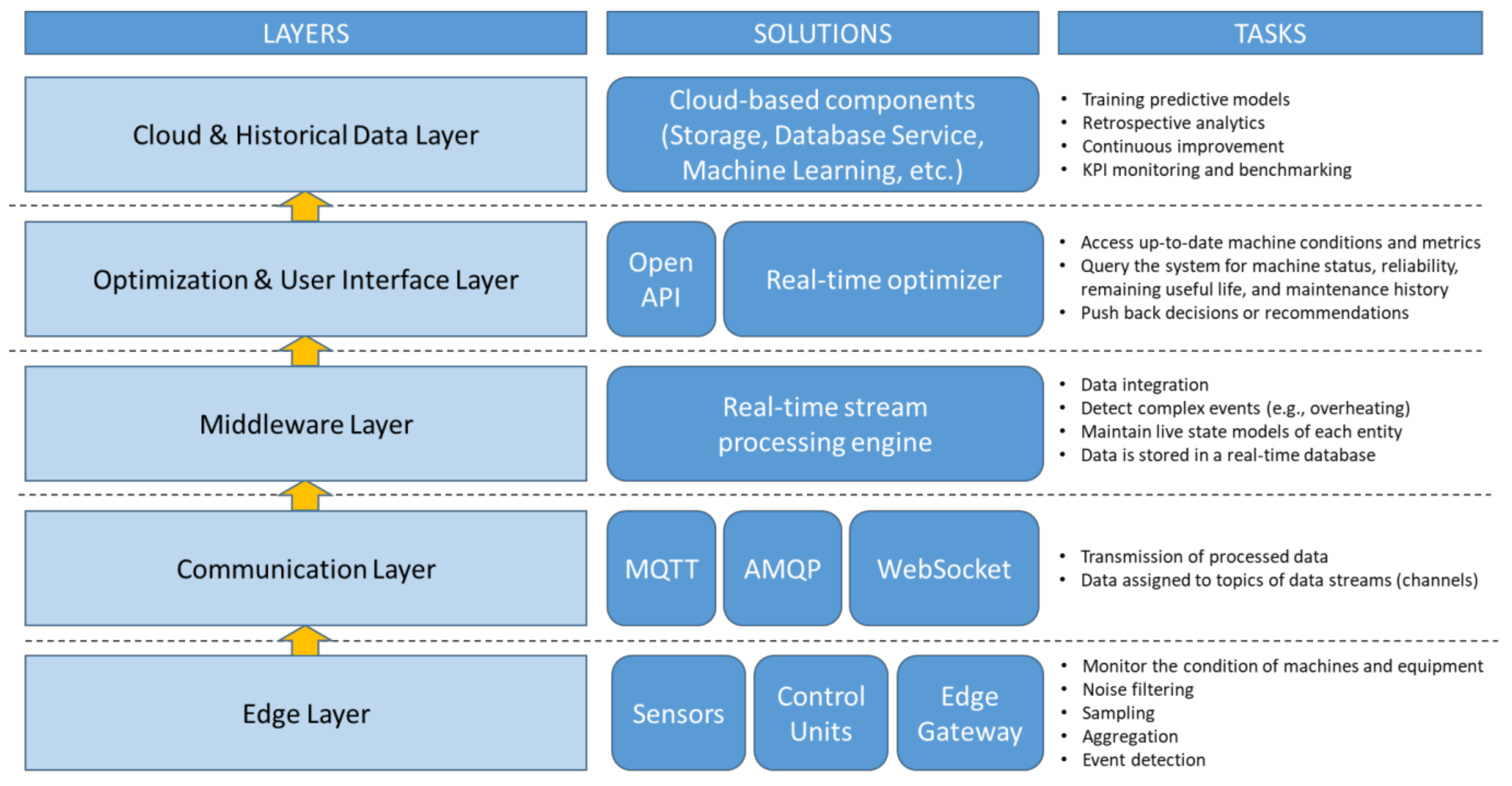
A general IIoT architecture suitable for collecting real-time state information from a production system and supplying relevant data to a real-time optimization software consists of several integrated layers (see Figure 1).

The system begins with an edge layer, where sensors and control units are installed on production equipment to continuously monitor parameters such as temperature, pressure, vibration, runtime, and fault signals. These devices are connected to an edge gateway that performs basic local preprocessing, including noise filtering, data aggregation, sampling, and real-time event detection (e.g., exceeding critical thresholds or detecting abnormal behavior).

The processed data are then transmitted through a real-time communication protocol such as MQTT, AMQP, or WebSocket to a centralized processing system. Data are structured into well-defined channels or topics, enabling organized, hierarchical data flow.

This is followed by a middleware layer responsible for integrating and processing the incoming data streams. A real-time data engine at this layer can detect significant events, maintain dynamic state models for each machine (such as condition index or reliability score), and store recent data in a high-performance, real-time or time-series database.

The optimization layer accesses this information through an open API, typically RESTful or WebSocket-based. Real-time optimization algorithms can query the system to retrieve the latest state of equipment, reliability indicators, maintenance history, or operational constraints. These algorithms can also send back decisions or recommendations, such as rescheduling tasks or initiating maintenance actions.

Optionally, a cloud-based component may be integrated to handle long-term data storage. This supports machine learning applications, historical analysis, and KPI tracking, helping the system to evolve over time and enabling advanced analytics for process improvement. Overall, this IIoT architecture ensures continuous feedback between the physical production environment and intelligent optimization tools, enhancing decision-making and operational efficiency.

3.3. Real-Time Maintenance Strategy Optimization in IIoT-Supported Production Systems

If the IIoT framework outlined in Section 3.2 is available, it is possible to transform the mathematical model presented in Section 3.1 into a real-time optimization model, which can be used to determine optimal maintenance parameters in real time. Since real-time optimization is fundamentally based on the conventional model presented in Section 3.1, only those elements that show significant differences from the conventional model will be presented.

The general structure (topology) of the production system can be described in the same way, as shown in Table 1. The input parameters are the same: layout configuration, degradation rate parameters, initial condition of the system component, and the impact of maintenance on the entity’s state. Regarding the input parameters, the most important difference is that the real-time state information of all entities in the manufacturing system is known during operation from the optimization and user interface layer.

The initial reliabilities of the three main types of nodes (entities, serial, and parallel connected entities) can be calculated using the same recursive algorithm, based on Equation (3). Based on the real-time state information, real-time decision-making can be performed to find the optimal maintenance performance for the next maintenance period. Based on this real-time decision, the reliability of the nodes and the reliability of the system, depending on the length of the maintenance period, assigned to maintenance period p, can be calculated. The following equation defines this iterative and recursive formula in the case of exponential degradation to calculate the state of a node in the iteration step p before maintenance:

$$r_{NODE}^{pPREM}=\left[\begin{array}{cc}{r}_i^{p-1}\left(s_i^{p-1}\right)+e^{-{DRP}_i·{\tau }_p^{*}},& iftheNODEismachinei\\ {\prod }_{i=1}^n{r}_i^{p-1}\left({child}_i^{p-1}\right)+e^{-{DRP}_i·{\tau }_p^{*}},& iftheNODEisaserialconnection\left(SER\right)\\ 1-{\prod }_{i=1}^n\left(1-r_i^{p-1}\left(s_i^{p-1}\right)+e^{-{DRP}_i·{\tau }_p^{*}}\right),& iftheNODEisaparallelconnection\left(PAR\right)\end{array}\right..$$

(8)

where ${\tau }_p^{*}$ is the length of the maintenance period for period p.

We can use Equation (9) as an iterative recursive formula to compute the reliability of the nodes and the reliability of the system for each maintenance period. The following equation defines this iterative and recursive formula:

$$r_{NODE}^{pPOSTM}=\left[\begin{array}{cc}{r}_i^{p-1}\left(s_i^{p-1}\right)+e^{-{DRP}_i·{\tau }_p^{*}}+{\delta }_i,& iftheNODEismachinei\\ {\prod }_{i=1}^n{r}_i^{p-1}\left({child}_i^{p-1}\right)+e^{-{DRP}_i·{\tau }_p^{*}}+{\delta }_i,& iftheNODEisaserialconnection\left(SER\right)\\ 1-{\prod }_{i=1}^n\left(1-r_i^{p-1}\left(s_i^{p-1}\right)+e^{-{DRP}_i·{\tau }_p^{*}}+{\delta }_i\right),& iftheNODEisaparallelconnection\left(PAR\right)\end{array}\right..$$

(9)

We have chosen the described recursive-iterative algorithm because it makes it possible to simulate the impact of real-time decisions during the optimization process. This enables the development of an optimal maintenance strategy in real time, ensuring that the reliability of both system components and the entire system is maintained at an optimal level, while also taking cost optimization into account. The recursive nature of the model reflects the fact that the reliability of subsystems and the entire system can be determined recursively based on the reliability of individual components. In contrast, the iterative nature of the model expresses that the system state is determined iteratively as a function of time.

In the case of this real-time maintenance strategy optimization model, the decision variables are the lengths of maintenance cycles for each period (${\tau }_p^{*}$). The described problems can be solved using a real-time optimizer, Section 4.2 shows the numerical results supported by an OpenSolver-supported simulation.

Various solvers are available for optimization tasks, ranging from commercial software to open-source solutions. OpenSolver, a free add-in for Microsoft Excel, offers a robust platform for solving linear, integer, and nonlinear optimization problems. Other widely used solvers, such as Gurobi 12.0.2 and CPLEX 22.1.2, are renowned for their high-performance capabilities but often require licensing fees. OpenSolver offers several key advantages, making it an attractive choice for optimization tasks. First and foremost, it is a cost-effective solution, as it is completely free to use, eliminating the need for expensive commercial solvers. Its seamless integration with Microsoft Excel is another significant benefit, as it allows users to directly solve optimization problems within their existing spreadsheet models without needing to switch between different platforms or tools.

We have included a summary table listing the key hyperparameters used in the Solver configuration (see

Table 2. Hyperparameters and settings used in the GRG nonlinear Solver.

Hyper Parameter	Description	Value
Convergence	Threshold for stopping optimization when changes in the objective are minimal	0.0001
Derivatives calculation method	How derivatives are approximated	Forward
Use multiple starting points	Enables global search by starting from multiple initial guesses	Disabled
Population size	Number of different initial guesses used if multistart is enabled	100
Random seed	Seed value for random number generation (for reproducibility)	0
Require bounds on variables	Ensures each decision variable has upper and lower bounds when using multistart	Enabled

). These parameters influence optimization behavior, convergence, and the risk of local vs. global optima. The default values were used unless stated otherwise.

4. Results

In this section, we provide a description of the experimental results based on the above-mentioned models and methods, their interpretation, as well as the experimental conclusions that can be drawn. The experimental results can be divided into three main parts. The first part discusses the optimization results of conventional maintenance, while the second part focuses on the IIoT-supported solution, where the design and control of maintenance operations are based on real-time optimization. In the third sub-section, the numerical results of both models are compared, and the experimental conclusions are drawn.

4.1. Optimization of Conventional State-Based Maintenance Operations

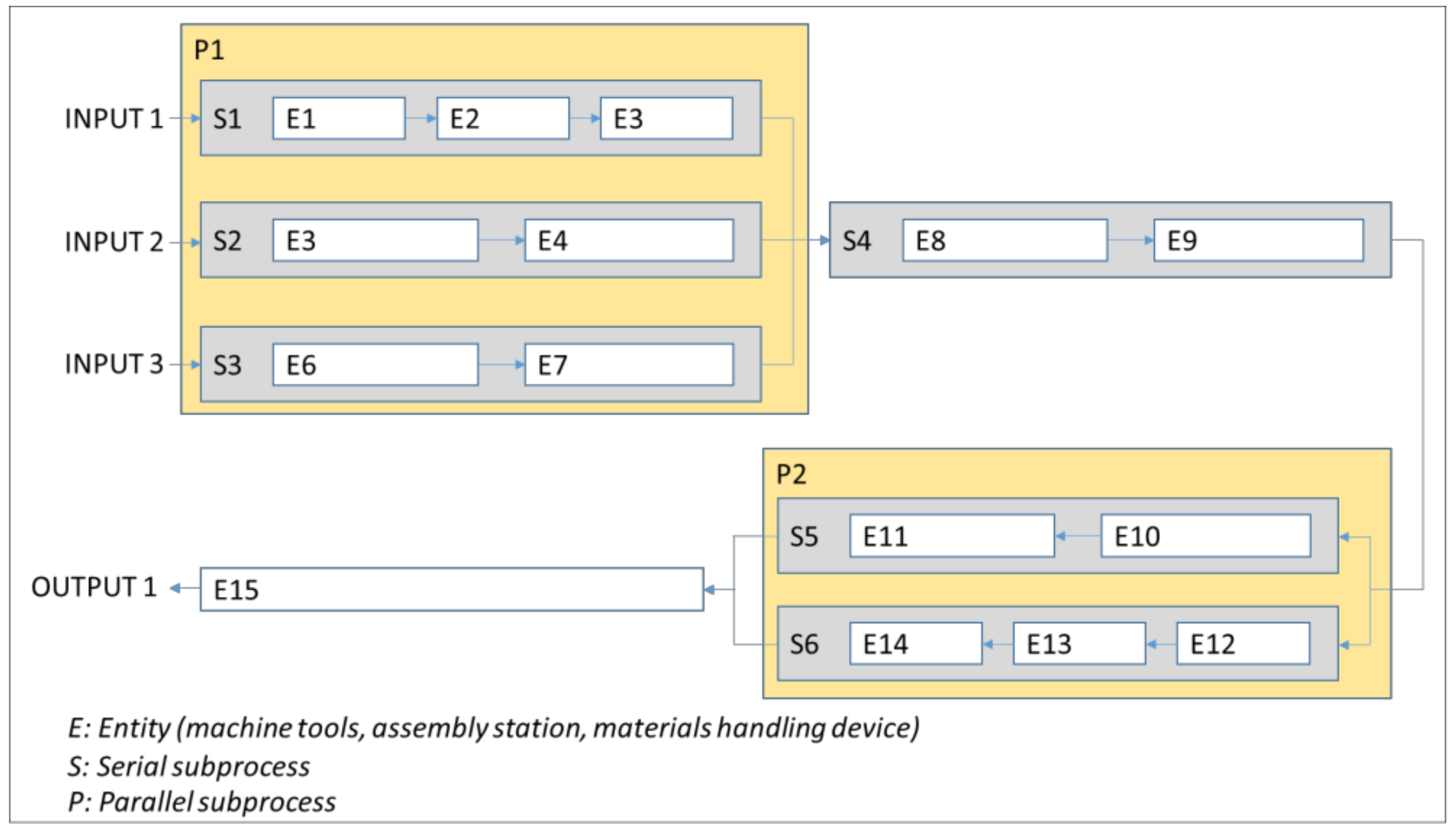
The analyzed production system includes 15 entities. In this case, study, these entities represent machine tools and assembly stations. Although the resources responsible for material handling and transportation are not marked separately, the case study explains how to take them into account. The entities within the production system are connected in both serial and parallel configurations, which defines the structure of the production process. Figure 2 shows the structure of the analyzed production system.

The mathematical description of the structure (layout) of the production system is defined as shown in

Table 3. Parent–child relationships of resources.

ID	Type	Child 1	Child 2	Child 3	Child 4	Initial State	Degradation Rate Parameter
E1	Entity					0.980	$3.3\times {10}^{-2}$
E2	Entity					0.985	$3.4\times {10}^{-2}$
E3	Entity					0.950	$2.9\times {10}^{-2}$
S1	Serial	E1	E2	E3		0.917
E4	Entity					0.992	$3.4\times {10}^{-2}$
E5	Entity					0.960	$2.8\times {10}^{-2}$
S2	Serial	E4	E5			0.873
E6	Entity					0.994	$2.9\times {10}^{-2}$
E7	Entity					0.990	$3.7\times {10}^{-2}$
S3	Serial	E6	E7			0.984
P1	Parallel	S1	S2	S3		1.000
E8	Entity					0.962	$3.3\times {10}^{-2}$
E9	Entity					0.982	$3.1\times {10}^{-2}$
S4	Serial	E8	E9			0.945
E10	Entity					0.961	$3.7\times {10}^{-2}$
E11	Entity					0.975	$2.6\times {10}^{-2}$
S5	Serial	E10	E11			0.937
E12	Entity					0.951	$4.1\times {10}^{-2}$
E13	Entity					0.988	$3.7\times {10}^{-2}$
E14	Entity					0.960	$3.6\times {10}^{-2}$
S6	Serial	E12	E13	E14		0.902
P2	Parallel	S5	S6			0.994
E15	Entity					0.986	$3.5\times {10}^{-2}$
S7	Serial	P1	S4	P2	E15	0.980

E: entity, S: serial, P: parallel.

. Table 3 defines parent–child relationships according to the recursive method described in the previous section. Table 3 also shows the basic degradation rate, which is a function of operation time.

We modeled the state of each entity using an exponential distribution. This choice is widely used in production system simulation studies due to its simplicity. The exponential distribution assumes a constant failure or transition rate, which is a reasonable approximation for many technical systems during their useful life phase. It also allows for the efficient simulation of random events such as failure times, repair times, time between breakdowns, service times, arrival times in queues, system response times, component lifetimes, and inter-arrival times in Poisson processes. By applying this model, we can realistically capture the stochastic behavior of the system without introducing unnecessary complexity.

In both numerical studies (simulation), we have chosen the following parameters for the calculation of the value of the objective function:

• the initial income generated by the production operations of the production system: $c_{SYS}^{PROD}=2000\mathrm{U}\mathrm{S}\mathrm{D}$
• the initial maintenance cost: $c_{SYS}^{MAIN}=1200\mathrm{U}\mathrm{S}\mathrm{D}$
• influencing factor, which defines the characteristics of the relationship between the reliability and the income, depending on the productivity: $\vartheta =0.5$
• influencing factor, which defines the characteristics of the relationship between the length of the maintenance period and the specific maintenance costs: $\epsilon =0.1.$

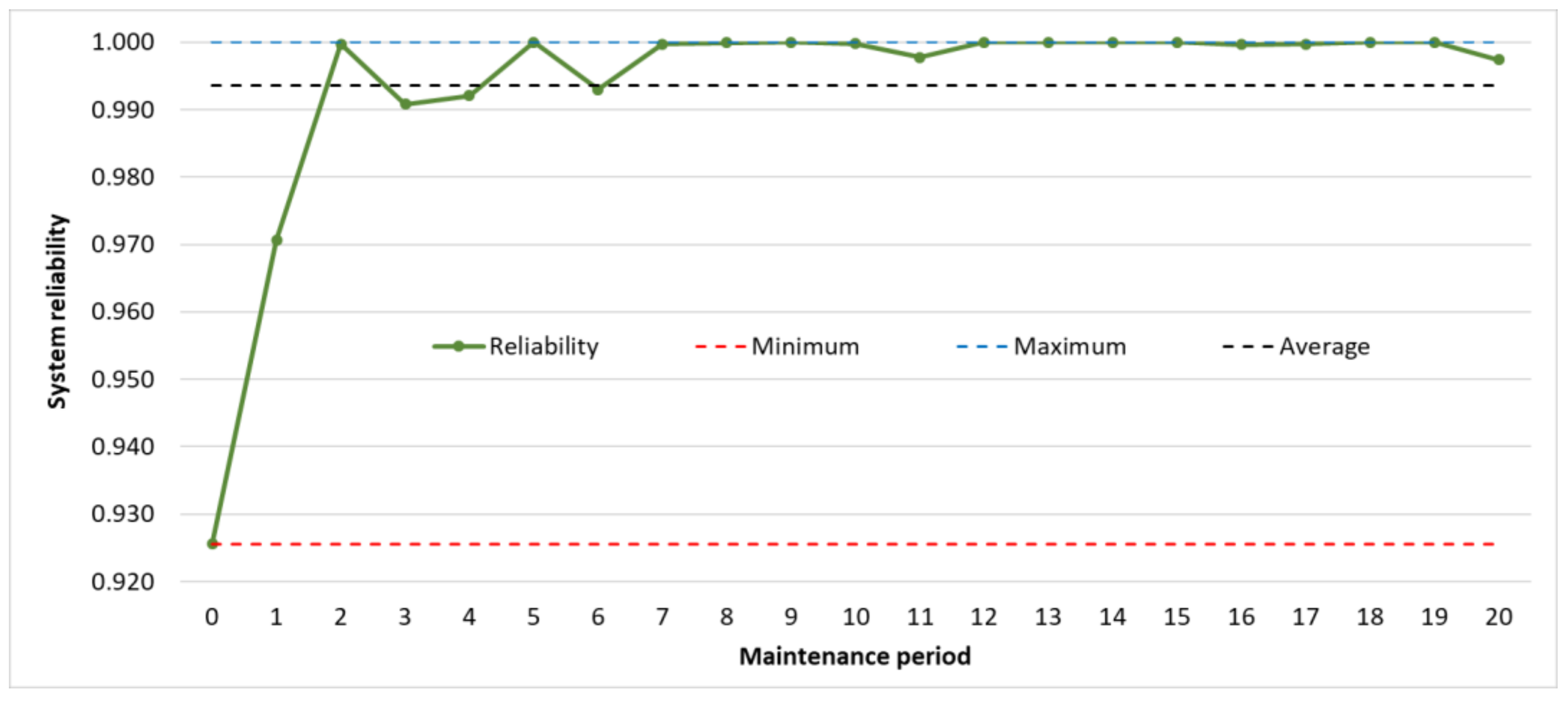
If maintenance is performed at regular intervals, one of the most important optimization parameters is the selection of the optimal maintenance intervals. Based on the mathematical model outlined in the previous section, it is possible to determine the optimal maintenance intervals in the current case study as well. Regular maintenance helps improve the reliability and overall performance of the system. Therefore, choosing the right maintenance frequency can significantly impact system efficiency. Let us examine how system reliability changes over time. The goal is to evaluate how different maintenance intervals affect the overall reliability of the system during this period. We have examined the impact of maintenance periods on system reliability in three different cases. In our model, we take 20 maintenance periods into consideration.

If the length of the maintenance period is 2.6 h, it often occurs that the system’s reliability reaches 100%, which suggests that unnecessary maintenance activities were performed, leading to additional costs (see Figure 3).

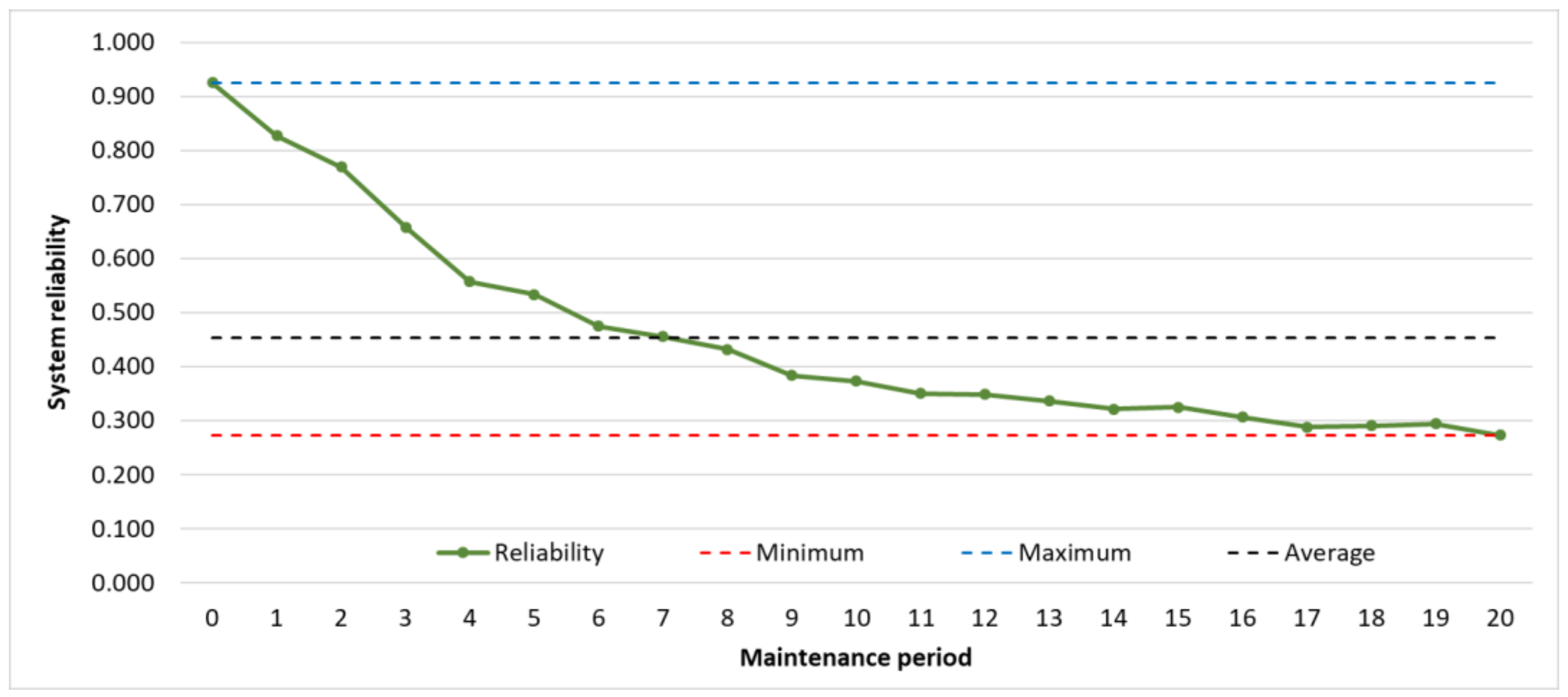
If the length of the maintenance period is 4 h, the system’s reliability never reaches 100%. As illustrated in Figure 4, the reliability of the system consistently decreases over time, which suggests that the 4 h maintenance cycle is not optimal for maintaining the system’s performance. This extended maintenance period is too long to ensure the system’s continuous productivity and efficiency.

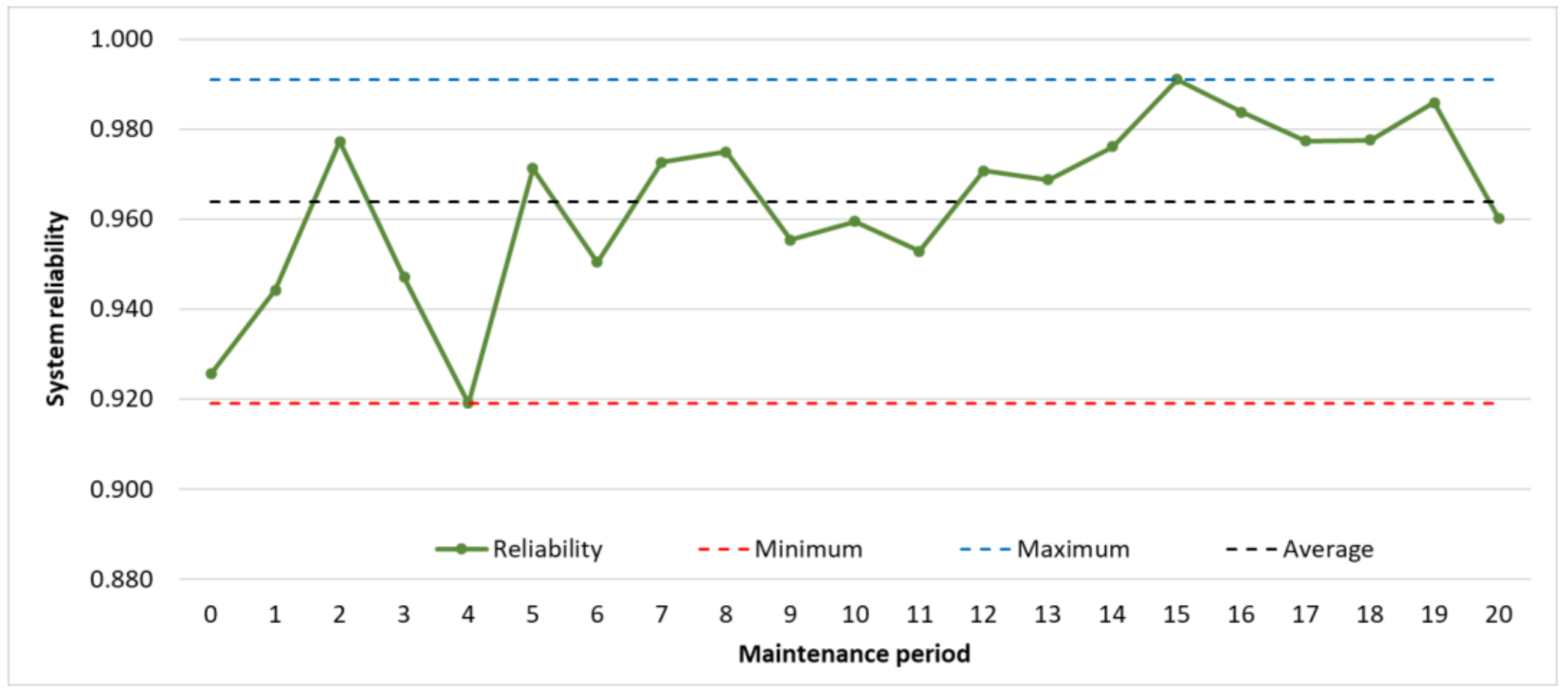
If the length of the maintenance period is 3 h, it rarely happens that the system’s reliability reaches 100%, which indicates that the 3 h long maintenance period is a significantly more cost-effective solution than the more frequent 2.6 h and less frequent 4 h long maintenance periods (see Figure 5).

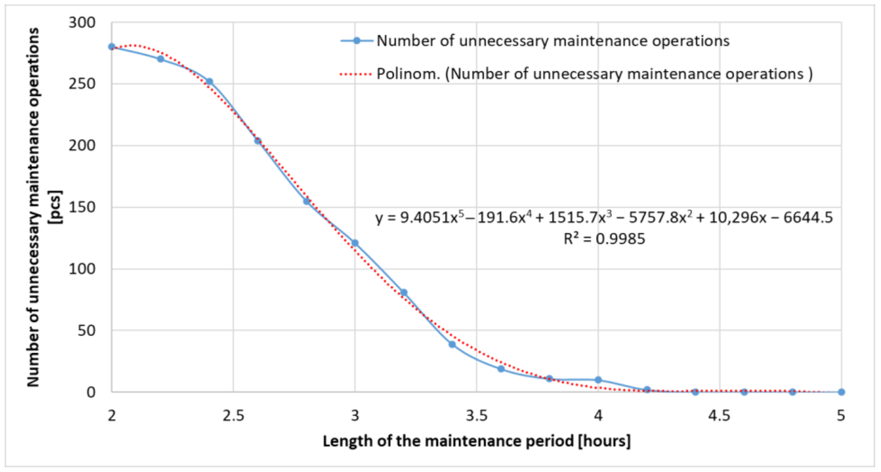
The other objective is to analyze the number of unnecessary maintenance operations (see Figure 6). It is important, because performing maintenance on a technical device that is in good condition can be counterproductive, as it may lead to unnecessary downtime and increased costs. Over-maintenance can also cause wear and tear on parts that are otherwise functioning properly, potentially reducing the lifespan of the equipment. Furthermore, unnecessary maintenance operations can disrupt the normal (productive) operation and efficiency of the system, leading to a loss of productivity.

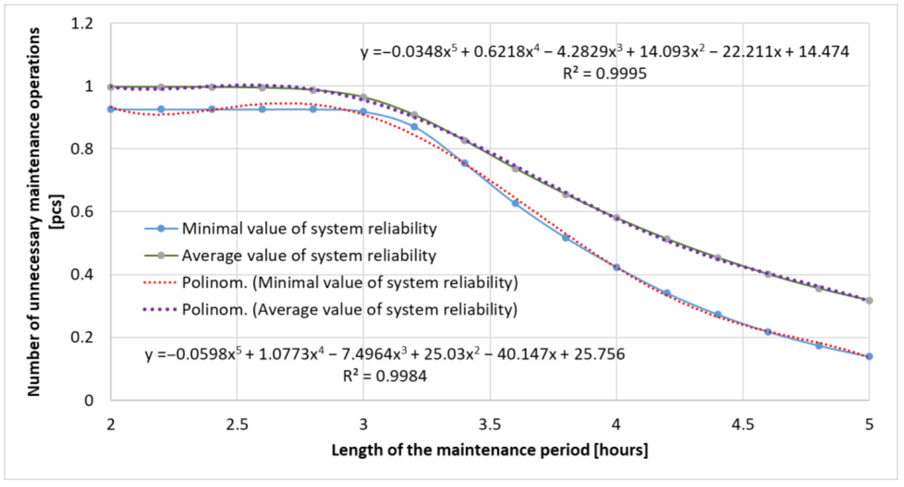
By examining the impact of maintenance periods on the system’s minimum and average reliability, it can be concluded that the more frequent the maintenance, the higher the minimum and average reliability values of the system. The relationship between the maintenance intervals and the system’s minimum and average reliability can be modeled using a fifth-degree polynomial with a coefficient of determination value of $R^2>0.99$. This indicates a strong correlation between the maintenance frequency and the system’s reliability (see Figure 7). As maintenance intervals decrease, the system’s reliability improves, reducing the risk of failures. Therefore, more frequent maintenance contributes significantly to enhancing both the minimum and average reliability of the system, but it can lead to significantly increasing costs and idle times.

It is worth analyzing how the length of the maintenance period influences the maintenance-related costs, the productivity resulting from system availability, and the income that can be determined as a result of these factors within the selected time window of the analysis. If the length of the maintenance period decreases, the cost of maintenance should also decrease. The appropriate formula can be written as follows:

$$c\left(t\right)=c_0·t^{-\vartheta }$$

(10)

where $c\left(t\right)$ is the cost of maintenance as a function of the length of the maintenance period, $c_0$ is the initial base maintenance cost (when $t=1$), and $\vartheta$ is a positive parameter that determines how much the cost decreases as maintenance becomes more frequent (the more often maintenance is performed, the cheaper each maintenance operation becomes).

In this formula, as the cycle time decreases, the maintenance cost also decreases. The parameter $\vartheta$ controls how rapidly the cost decreases with shorter cycle times. For example, if $\vartheta =1$, the cost is inversely proportional to the cycle time, meaning that the more frequently maintenance is performed, the lower the cost per maintenance. If $\vartheta$ is greater, the cost decreases more rapidly.

We can use the same logic to define the relationship between productivity and reliability of the system. A possible equation is the following:

$$p\left(r\right)=p_0·r^{\alpha }$$

(11)

where $p\left(r\right)$ is the productivity of the production system as a function of its reliability, $p_0$ is the maximum available productivity (when the production system operates with 100% reliability), $r$ is the system’s reliability, ranging from 0 to 1, and α is a parameter that determines how strongly reliability affects productivity.

Based on these two equations, it is possible to calculate the maintenance cost for the analyzed time window, the income related to the productivity of the analyzed production system, and the profit depending on the maintenance cost and the income based on productivity. The relationship between the maintenance intervals and the profit, depending on the maintenance cost and the income based on productivity, can be modeled using a third-degree polynomial with a coefficient of determination value of $R^2>0.99$. Figure 8 shows the relationship between the maintenance periods and the specific profit depending on the maintenance cost and the income based on productivity.

4.2. IIoT Technologies-Supported Real-Time Optimization of Maintenance Operations

The conventional maintenance optimization solution outlined in Section 4.1 has the disadvantage that maintenance tasks for different system components (entities) are carried out based on a predefined or optimized maintenance period (cycle time). The advantage of this approach is its simplicity and predictability, as maintenance operations occur at regular intervals. However, if real-time data from the system’s structural resources (production and logistics resources) are available, maintenance activities can be optimized by eliminating unnecessary maintenance operations, ensuring that only necessary maintenance is performed. At the same time, this approach ensures that the system’s reliability remains at a level that guarantees required productivity. Real-time optimization based on these data forms the foundation of the IIoT-based solution presented in the previous chapter. In this IIoT-based real-time optimization model, the input data are the same as the input data used in the case study demonstrating the conventional optimization task (see Figure 2 and Table 3).

If real-time state information of the manufacturing system’s resources is available, it is possible to determine the optimal maintenance period in real-time, taking this information into account. The maintenance period is dynamically changing within the time window of the analysis. Using the mathematical model presented in Section 3.1, real-time optimization simulation can be performed in the production system defined by Figure 2 and Table 3. The results of this simulation are illustrated in Figure 9, Figure 10 and Figure 11.

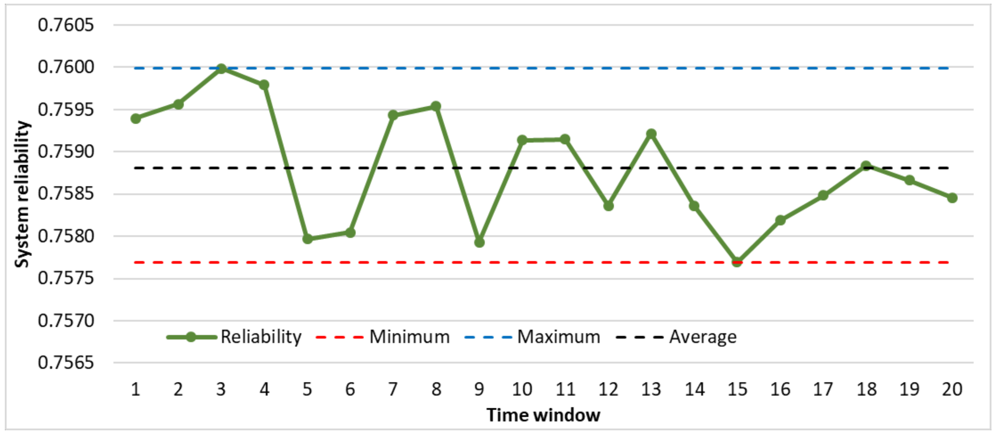
Figure 9 illustrates the case where the length of each maintenance period must be optimized in real-time in such a way that the reliability of the manufacturing system does not fall below 60%. In this case, the minimum length of the optimized maintenance periods is 3.175 h, the average length is 3.712 h, the maximum length is 6.725 h, while the standard deviation is 0.752 h. In this case, the analyzed 20 maintenance periods covered 74.25 h of production time.

Figure 10 illustrates the case where the length of each maintenance period must be optimized in real-time in such a way that the reliability of the manufacturing system does not fall below 75%. In this case, the minimum length of the optimized maintenance periods is 2.925 h, the average length is 3.452 h, the maximum length is 5.05 h, while the standard deviation is 0.462 h. In this case, the analyzed 20 maintenance periods covered 69.05 h of production time.

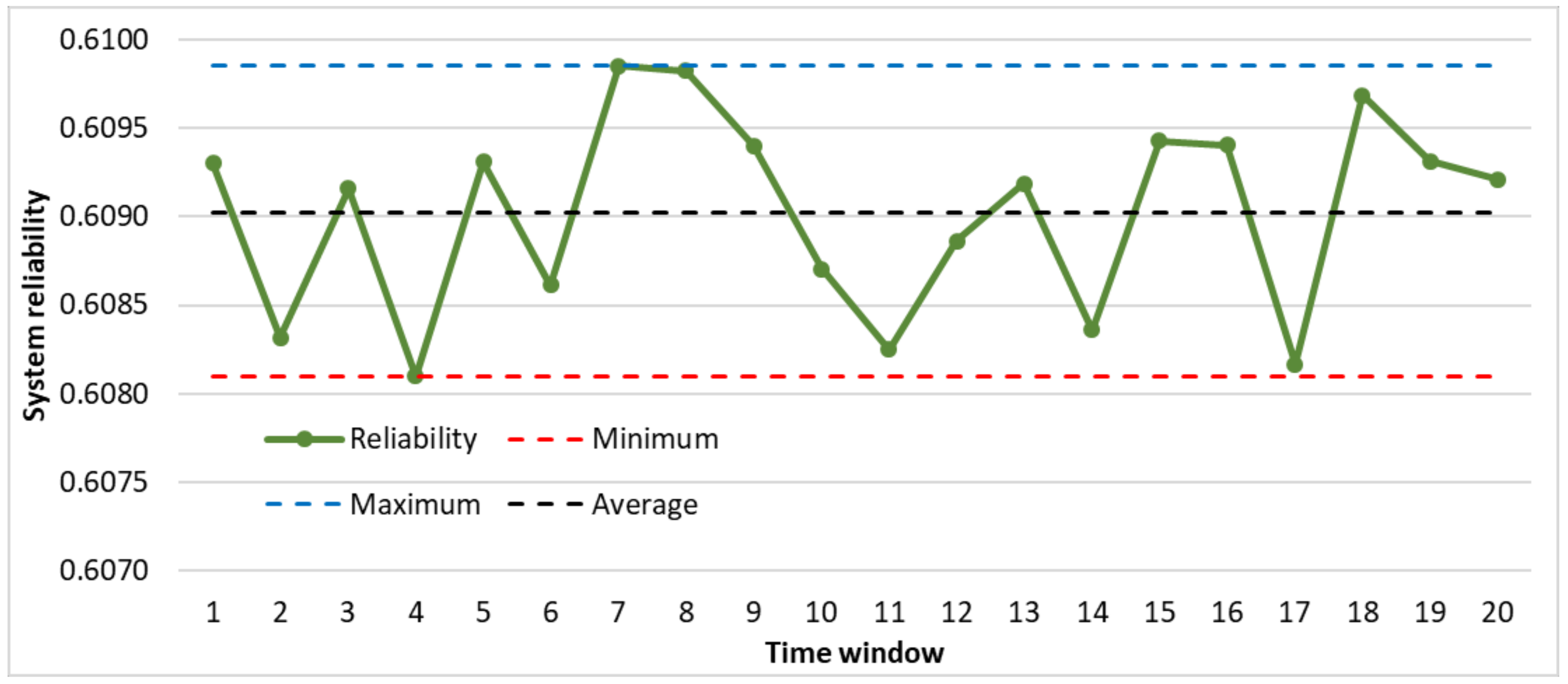
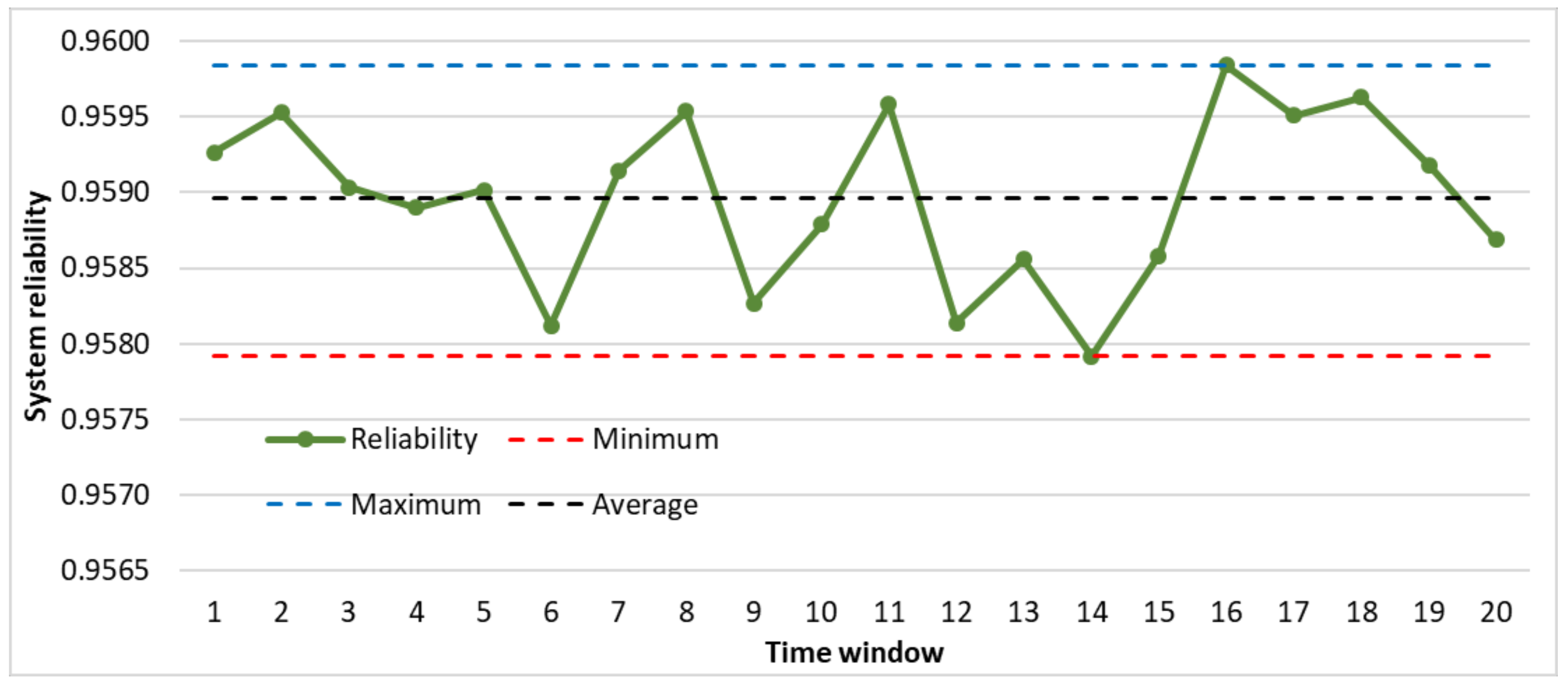
Figure 11 illustrates the case where the length of each maintenance period must be optimized in real-time in such a way that the reliability of the manufacturing system does not fall below 95%. In this case, the minimum length of the optimized maintenance periods is 2.6 h, the average length is 3.099 h, the maximum length is 3.725 h, while the standard deviation is 0.314 h. In this case, the analyzed 20 maintenance periods covered 61.97 h of production time.

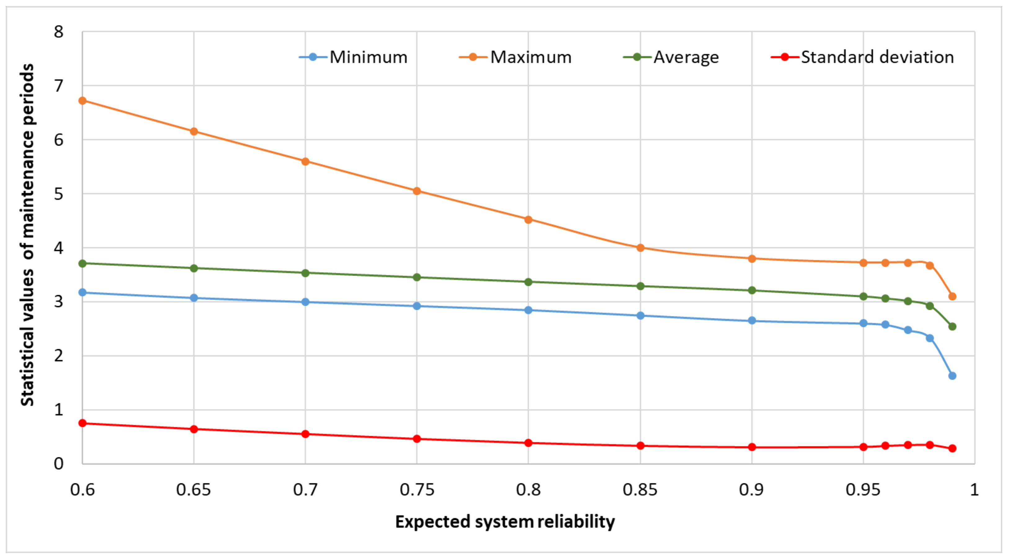
By analyzing the characteristics of the maintenance periods in detail (see Figure 12), it can be clearly observed that an increase in the predefined minimum system reliability results in a notable reduction in the statistical parameters of the maintenance periods, including their minimum, maximum, average, and standard deviation values. This implies that the higher the reliability requirement, the more consistent and shorter the maintenance intervals become. Furthermore, the rate of this reduction becomes increasingly steep once the minimum system reliability surpasses the 95% threshold, indicating a nonlinear relationship. In this critical range, even small increases in the reliability constraint cause disproportionately large decreases in the variability and length of the maintenance periods, highlighting the sensitivity of the system to high-reliability demands in real-time optimization scenarios.

Figure 13 shows how the number of production hours covered by 20 maintenance periods changes as a result of real-time optimization simulation, depending on the expected system reliability within the range of 60% to 99%. The simulation demonstrates that as the expected reliability increases, the total production time that can be maintained without exceeding the reliability threshold generally decreases. This trend theoretically reflects the increasing need for more frequent or shorter maintenance intervals to preserve higher levels of reliability, if required. To describe the relationship between the expected system reliability and the number of production hours, a sixth-degree polynomial function provides a suitable fit. The coefficients of the polynomial regression were calculated using the least squares method based on the observed data, with the polynomial degree selected to balance model complexity and accuracy. The resulting R² value is greater than 0.98, confirming an excellent fit without signs of overfitting.

In the next step, let us examine how the maintenance periods calculated by real-time optimization, based on dynamically changing real state data, affect the specific maintenance cost for a maintenance period, the specific income related to the productivity of the analyzed production system, and the specific profit depending on the maintenance cost and the income based on productivity. Figure 14 shows the results of this analysis in the case of $r_{min}=0.6$, while Figure 15 shows the results in the case of $r_{min}=0.95$.

As Figure 14 shows, real-time optimization enables the development of maintenance periods that significantly contribute to maintaining a stable reliability of $r_{min}=0.6$ within the production system. This is achieved by dynamically calculating the maintenance periods based on the real-time state information of the production system in real-time. Consequently, these periods are continuously adjusted within the analysis time window, reflecting the ever-changing state of the system.

In this case, the total production time covered by 20 maintenance operations is 74.25 h, the total income is 30,983 USD, the total maintenance cost is 7529.5 USD, while the total profit is 23,454.5 USD. The hourly profit is 315.88 USD.

Figure 15 shows the same results in the case of $r_{min}=0.95$.

In the case of $r_{min}=0.95$, the total production time covered by 20 maintenance operations is 61.975 h, the total income is 38,987 USD, the total maintenance cost is 8744.7 USD, while the total profit is 30,242.3 USD. The hourly profit is 487.97 USD.

This approach leads to a dynamically varying specific maintenance cost, as the timing and necessity of maintenance operations evolve alongside system conditions. As a result, a time-profit function can be calculated, which, due to the relatively stable revenue generated from productivity, closely reflects the characteristics of the specific maintenance cost over time. This demonstrates how the integration of real-time state information into the optimization process not only enhances system stability but also allows for cost-sensitive and responsive maintenance planning.

4.3. Experimental Conclusions

Based on the comparison of the results of conventional and real-time optimization, the following experimental conclusions can be drawn:

• In the case of real-time optimization, the same number of maintenance operations can result in a longer production time, as maintenance operations that are not justified by the condition of the system or its resources are not carried out (i.e., the condition of the system or a resource does not reach a threshold that would necessitate a maintenance operation). As a result of real-time optimization, the 20 maintenance cycles examined in the case study allowed for a 12% longer production time (see

  Table 4. Comparison of the main parameters of conventional and IIoT-supported real-time optimization-based maintenance strategies.

  	Conventional				Real-Time
  	Length of Maintenance Periods				Reliability
  	2	3	4	5	0.6	0.95
  PT20 1	60	60	60	60	74.25	61.975
  TI20 2	19,245.77	12,781.93	6511.53	2982.61	30,983	38,987
  TMC20 3	6430.64	2976.32	1723.05	1127.63	7529.5	8744.7
  TP20 4	12,815.13	9805.61	4788.48	1854.98	23,454.5	30,242.3
  HP 5	213.59	163.43	79.81	30.92	315.88	487.97

  ¹ Production time covered by 20 maintenance periods. ² Total income over 20 maintenance periods. ³ Total maintenance cost over 20 maintenance periods. ⁴ Total profit over 20 maintenance periods. ⁵ Hourly profit.

  );
• In the case of real-time optimization, the income calculated from productivity increases significantly, as constant reliability can be ensured through maintenance operations optimized in real time, thanks to continuous monitoring of the system’s condition. As a result of real-time optimization, the revenue calculated from productivity in the system outlined in the case study almost doubled (see Table 4);
• In the case of real-time optimization, maintenance costs increased by 17% to 775% (see Table 3). This increase is due to the fact that the changing maintenance periods require significant flexibility from the maintenance department, which results in additional costs. Although maintenance costs can increase substantially, the high level of productivity resulting from the stable reliability of the manufacturing system generates revenue that more than covers the increased maintenance expenses. This is supported by the calculated profit;
• In the case of real-time optimization, the profit calculated from productivity-based revenue and maintenance costs increased. In the case study, this increase ranged from 2.5 to 12 times (see Table 4), confirming that real-time maintenance optimization based on IIoT technologies can bring significant economic benefits.

5. Discussion

This study presents a novel real-time maintenance optimization approach that integrates Industrial Internet of Things (IIoT) technologies with real-time, adaptive optimization. Unlike previous studies primarily focusing on anomaly detection or early fault identification, our method goes a step further by actively optimizing maintenance actions in real time based on continuous feedback from the system. One major distinction lies in the depth of real-time optimization: while existing studies typically stop at detection, our model supports continuous decision-making to improve performance and reduce costs. For instance, Katib et al. (2025) emphasize anomaly detection in consumer IoT devices using TinyML and deep learning, but do not address dynamic optimization [20]. In contrast, we propose a mathematical model that uses IIoT data to adaptively minimize maintenance costs while maximizing system efficiency. For example, consider a CNC milling machine used in automotive component manufacturing, equipped with several IIoT sensors to monitor its performance. The IIoT system collects various data types, including vibration data from accelerometers placed on the spindle and bearing housings, with a sampling interval of every 10 s for continuous monitoring. Temperature data are gathered from sensors on the spindle and motor, averaged every minute. Additionally, current consumption is measured on the main motor and tool drive, with readings taken every 5 s. Finally, operational time and cycle count are tracked by the machine controller and recorded per production cycle. The mathematical model utilizes these data to predict the likelihood of failure for critical components such as the spindle or bearings using machine learning techniques like decision trees or logistic regression. By integrating these predictions, the model helps optimize the timing of maintenance tasks. It balances the cost of preventive maintenance with the cost of failure, ensuring maintenance is only performed when necessary. The model works by minimizing a cost function that incorporates both maintenance and failure costs. As a result, maintenance is no longer scheduled at fixed intervals. Instead, the model triggers maintenance only when the data signals an increased risk of failure. Mohapatra et al. (2024) apply IoT and the Analytic Hierarchy Process (AHP) to prioritize parameters in diesel generator systems, but lack a dynamic, real-time optimization layer [21]. Ayvaz and Alpay (2021) use machine learning models for early failure detection [22], and Arockiasamy et al. (2023) offer a literature review on sensor-enabled composites [23], but both primarily focus on monitoring and detection rather than integrated optimization. The existing studies are largely data-driven, applying machine learning or statistical techniques, whereas our approach combines data with a model-driven framework for more strategic and intelligent decision-making. This allows us not only to predict failures but also to plan maintenance activities in real time with clear economic and operational objectives. Additionally, while prior work tends to focus on tactical-level challenges such as short-term fault prevention, our study considers maintenance as a strategic tool for improving production efficiency and long-term performance. This makes our solution particularly well suited for smart factory environments where maintenance must align with broader industrial goals. Moreover, our model is designed specifically for Industrial IoT applications, ensuring scalability and strong relevance to real-world manufacturing systems. Overall, the proposed approach transforms maintenance from a reactive or predictive task into a real-time, cost-effective, and system-wide optimization process, supporting the core objectives of Industry 4.0.

Advanced methods such as LSTM, neural networks, and 1D-CNNs are widely used in predictive maintenance, especially when large volumes of IoT sensor data are available. However, our goal was to explore a simpler, and more interpretable approach. While polynomial regression may not always outperform these complex models in general, in our case, it achieved a high coefficient of determination (R² > 0.98), indicating an excellent fit to the observed data. This suggests that for the type and amount of data we used, the polynomial model is sufficient and effective. We believe that such a lightweight method can be beneficial in scenarios where computational efficiency and transparency are important. In our study, raw data for polynomial regression were not derived from IIoT sensor data, but rather from structured data corresponding to the following use cases:

• the number of unnecessary maintenance operations as a function of the maintenance interval;
• the impact of maintenance period on the minimum and average value of system reliability;
• the relationship between the maintenance periods and the specific profit, depending on the maintenance cost and the income based on productivity;
• the relationship between expected system reliability and production hours covered by a predefined number of maintenance periods.

We would like to provide a brief example to demonstrate hands-on insights into the application of our IIoT framework, as follows. For example, consider a flexible manufacturing system, where CNC milling machines are used, and they are equipped with several IIoT sensors to monitor their performance. The IIoT system collects various data types, including vibration data from accelerometers placed on the spindle and bearing housings, with a sampling interval of every 10 s for continuous monitoring. Temperature data are gathered from sensors on the spindle and motor, averaged every minute. Additionally, current consumption is measured on the main motor and tool drive, with readings taken every 5 s. Finally, operational time and cycle count are tracked by the machine controller and recorded per production cycle. The mathematical model utilizes these data to predict the likelihood of failure for critical components such as the spindle or bearings using machine learning techniques like decision trees or logistic regression. By integrating these predictions, the model helps optimize the timing of maintenance tasks. It balances the cost of preventive maintenance with the cost of failure, ensuring maintenance is only performed when necessary. The model works by minimizing a cost function that incorporates both maintenance and failure costs. As a result, maintenance is no longer scheduled at fixed intervals. Instead, the model triggers maintenance only when the data signals an increased risk of failure.

6. Conclusions

The model is a general framework that, due to its recursive nature, can be applied to a wide range of system structures. Its flexibility allows it to be used in various cases regardless of the specific configuration of components. However, systems with bridge-type connections may represent an exception, as these structures can introduce dependencies that are not fully captured by the current recursive logic. Nonetheless, for most conventional system architectures, the model remains broadly applicable and effective.

This research introduces a novel real-time maintenance optimization framework that moves beyond traditional fault detection by integrating Industrial IoT data with adaptive, model-driven decision-making. Unlike previous studies, which focus primarily on monitoring or anomaly detection, our approach continuously adjusts maintenance strategies in real time to minimize costs and maximize system efficiency. A key innovation lies in transforming maintenance from a reactive or predictive task into a strategic, real-time optimization process that aligns with the broader objectives of Industry 4.0. The recursive and iterative structure of the model enables scalable application across diverse system architectures, offering a generalized solution suitable for smart factory environments. By embedding real-time optimization into safety assessment and risk management, the research enhances the responsiveness, reliability, and overall intelligence of maintenance operations in industrial systems.

Safety assessment from a maintenance perspective is a fundamental element of industrial risk management. It involves the systematic identification of potential hazards related to maintenance activities, such as equipment failures, human errors, or exposure to hazardous substances. Risk assessment quantifies the likelihood and consequences of these hazards, enabling the prioritization of preventive actions. Our proposed real-time maintenance optimization plays a key role in this process by supporting data-driven decision-making, allowing for the early detection of risks and rapid response. This approach significantly enhances the safety, reliability, and efficiency of maintenance operations.

Future research could explore the integration of real-time maintenance optimization with dynamic production scheduling to improve overall system coordination. Another promising direction is the development of multi-objective optimization models that balance cost, energy use, environmental impact, and safety. Enhancing the system’s ability to learn from past maintenance outcomes could improve decision-making over time. Finally, research on cybersecurity and data integrity will be essential to ensure the safe and reliable use of IIoT in industrial environments.