Predicting Clay Swelling Pressure: A Comparative Analysis of Advanced Symbolic Regression Techniques

Abstract

Swelling pressure is a key geotechnical property that influences the behaviour and stability of engineering structures built on expansive clayey soils. This pressure can be measured directly through laboratory tests or estimated using indirect methods. This paper analyses a dataset of undisturbed clay samples from southeastern Spain using advanced symbolic regression techniques, namely: deep symbolic regression (PhySO), high-performance symbolic regression (PySR), multi-objective symbolic regression (MOSR), and physics-guided symbolic regression (PGSR). These methods provide interpretable results as equations, unlike standard machine learning models. All generated equations showed high performance (R² > 0.91 and MAE < 23 kPa) and simplicity, making them suitable for practical engineering applications. PySR yielded the best overall metrics (R² = 0.933, MAE = 20.49 kPa), particularly excelling in high-pressure ranges, while PhySO demonstrated the most balanced performance, especially for low to medium pressures. MOSR minimized edge-case bias, and PGSR, despite lower overall performance, remained competitive. The plasticity index (PI) was identified as the most influential factor in all models, followed by the percentage of fines. The use of undisturbed samples enhanced the reliability of the findings, and the resulting equations enable a flexible estimation of swelling pressure based on commonly available geotechnical parameters.

1. Introduction

Swelling pressure (p_s) is a critical parameter in various fields, including geotechnical engineering [1]. It refers to the pressure exerted by a material when it expands upon absorbing a fluid, usually water. This phenomenon is particularly significant in the context of expansive soils, which can undergo substantial volume changes due to variations in moisture content. Expansive soils can pose significant economic costs due to their swelling and shrinking behaviours. These changes can lead to structural damage in buildings and infrastructure, resulting in a remarkably high cost, with the annual global expenditure on repairs estimated to reach several billion dollars [2,3]. Sabtan [4] indicated that the swelling behaviour is primarily influenced by the combined effect of several interacting factors, which can be categorized as: (a) local geology; (b) engineering properties; and (c) local environment of deposition. Geological factors encompass the rock type and age, which are related to the type and quantity of clay minerals, the type and amount of cementing material, and the arrangement of soil particles. Engineering factors include moisture content, Atterberg limits, and dry density. Environmental factors involve confining pressure, weathering type and degree, clay fraction content, initial water content, and water chemistry. While the swelling potential is influenced by geological and engineering factors, the amount and rate of swelling are governed by environmental conditions.

Expansive soils are widely distributed throughout the world, although they are especially abundant in arid zones, where conditions are suitable for the formation of clayey minerals of the smectite group such as montmorillonite or some types of illites [5]. In geotechnical practice, the determination of p_s is crucial for designing foundations and retaining structures, tunnels, and other geotechnical structures. Accurate predictions can facilitate the implementation of appropriate engineering measures to mitigate its effects and reduce costs in engineering projects [6,7]. There are different techniques applicable in this type of soil to mitigate its potential volume changes, essentially involving the addition of a stabilizing material (e.g., refs. [8,9,10,11]). Various laboratory tests, such as the oedometer test and the triaxial test, are commonly employed to directly measure p_s [12]. However, there are numerous correlations available that relate p_s to other easily obtainable geotechnical parameters [13]. Many researchers have extensively investigated the factors influencing soil swelling and have attempted to establish relationships between soil properties, including clay content, dry unit weight, water content, liquid limit, and plasticity index (e.g., refs. [4,14,15,16,17,18,19]). In the face of these challenges, the application of machine learning (ML) techniques can offer promising opportunities for advancing the understanding of clay swelling [20]. ML models can handle the complexity of the swelling process, making them powerful tools for predicting p_s based on a range of input parameters (e.g., refs. [21,22,23]). Gahlot et al. [24] provided a comprehensive review of the ML methods applied to obtain p_s. However, it is important to note that most traditional statistical correlations and existing ML algorithms are based on datasets of remoulded clay samples, where the soil structure is altered during both the extraction process and the compaction for testing. This reliance on remoulded samples may not accurately represent the behaviour of undisturbed soils, potentially limiting the applicability of these models to in situ soil conditions. Numerous studies (e.g., ref. [25]) have shown that correlations derived from remoulded samples can differ significantly from those based on undisturbed samples, highlighting the need for caution when applying such models to natural soil conditions.

Although effective, ML models often lack transparency (black boxes), posing challenges for specific applications or when dealing with new data categories. As a result, efficient analytical formulas and algorithms could be preferred [26]. Symbolic regression (SR), a machine learning approach, aims to automatically discover formulas that capture correlations within a given dataset [27], offering models in the form of easily understandable mathematical equations. While it has traditionally been implemented using Genetic Programming [28], alternative approaches also exist. These include deterministic methods that systematically explore the space of mathematical expressions, deep learning-based techniques, transformer-based methods, and hybrid algorithms that combine multiple strategies to enhance the efficiency and accuracy of SR, among others. SR has been used in geological and geotechnical engineering [29,30,31,32] and, specifically, to obtain p_s [33] with satisfactory results.

Despite the increasing number of studies addressing the prediction of p_s using empirical or machine learning approaches, several critical gaps remain. Firstly, most existing correlations are based on remoulded samples, which fail to reflect in situ conditions and may lead to misleading predictions. Secondly, widely used ML models often operate as black-box systems, lacking interpretability and offering limited insight into the influence of input parameters. Lastly, few studies have explored the use of SR algorithms that produce simple, physically meaningful equations while maintaining high predictive accuracy.

In response to these limitations, this study aims to explore the capabilities of SR as a tool to discover patterns in complex datasets in order to synthesize simple equations that allow engineers to estimate the p_s value in clayey soils with the same characteristics as those studied here, with a high degree of reliability. To achieve this, it is only necessary to know some easily obtainable index properties, such as: liquid limit (LL), plasticity index (PI), dry density (γ_d), percentages passing through a 0.075 mm sieve, and natural water content (w). Additionally, the most influential input variables on the final value of p_s were evaluated.

2. Study Area

In Spain, expansive soils cover approximately 30% of the territory and primarily belong to the montmorillonite group [34]. Additionally, 67% of the country is located in climates where significant moisture changes can occur in the soil, with dry periods ranging from two to eight months [35]. The study area is located in the southeastern region of Spain, specifically in the provinces of Murcia and Almería. Figure 1 presents the potential swelling risk map of Spain [35] along with the locations of the two primary sample sources used in this study. The samples were obtained in the context of different engineering projects, including road infrastructures, slope stability works, building structures, and foundation reinforcements for existing structures. As such, they are disseminated. In this way, the study areas were defined based on whether the samples belong to geotechnical units exhibiting similar swelling behaviours, according to the potential ranges established in Figure 1. As can be observed, the studied areas fall into the category of expansive clays with a moderate to high swelling potential (expected p_s between 125–300 kPa) and high to very high potential (expected p_s upper than 300 kPa). They consist of clayey–marly soils with medium-to-high plasticity and contain clays from the montmorillonite group, belonging to Neogene materials. According to the authors’ experience, they can achieve relatively high p_s values (above 400 kPa).

In the study area, there are numerous cities, as well as associated structures, roads, railway lines, and slopes. If adequate measures are not taken, all of these may experience pathologies due to cyclic swelling and shrinkage. Specifically, buildings can suffer differential settlement, triggering diagonal or stair-step cracks in walls and foundation displacement, particularly in lightweight structures with shallow footings. Slopes develop vertical or subvertical desiccation cracks during droughts, followed by superficial landslides upon wetting due to a reduction in shear strength. Roadways develop longitudinal cracks parallel to the direction of traffic due to differential heave between the centreline and shoulders. Concurrently, edge uplift occurs along rigid boundaries (e.g., medians, curbs) caused by moisture-induced swelling pressure gradients. In concrete pavements, differential heave or settlement causes edges or corners of the concrete slabs to lift or sink, creating uneven surfaces. This process induces cracks at slab edges or joints, as well as mid-slab longitudinal cracking, along with minor associated transverse cracks. 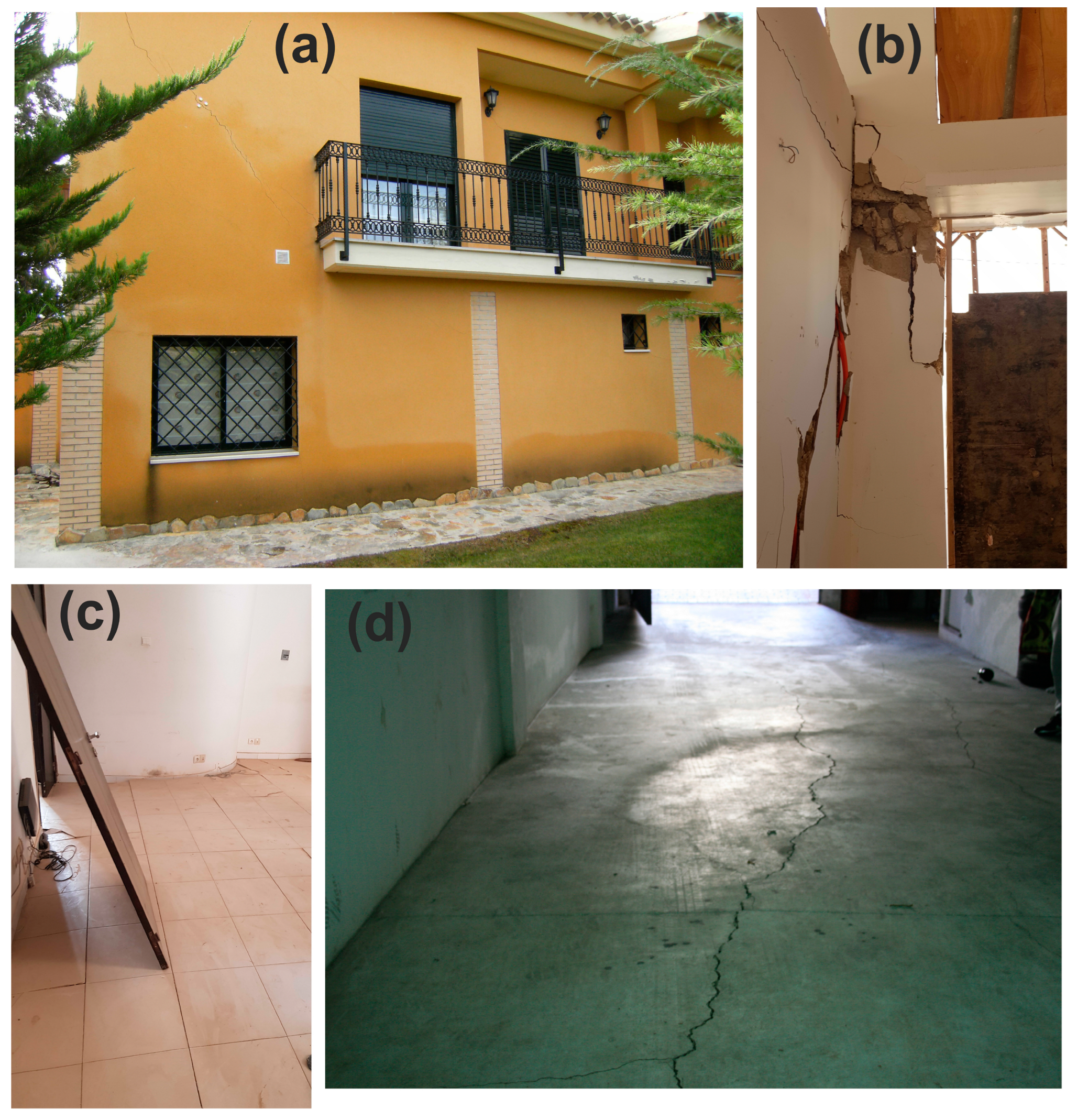Figure 2 shows damage in recently constructed structures on expansive clays, where the authors were involved in structural rehabilitation and underpinning work. In Figure 2a, typical cracks associated with soil expansion and shrinkage phenomena are observed, in this case at a 45° angle, with a crack monitor to track movement. Figure 2b presents a similar case, but with more severe damage due to the combined effect of highly expansive clays and construction defects. In Figure 2c,d, it can be seen how swelling affects the lighter parts of the structure such as rigid concrete floor slabs and garage slabs in direct contact with expansive clays.

This is, therefore, a very common problem that needs to be anticipated, with p_s being the most important parameter for its assessment. Likewise, when implementing the necessary reinforcement measures (e.g., underpinning), p_s remains the key soil-related factor for their design.

3. Experimental Studies

A total of 181 undisturbed clay samples were collected. These samples were tested in a laboratory, obtaining various geotechnical parameters, including LL, PI, γ_d, percentages passing through a 0.075 mm sieve, w, and p_s. A series of standardized tests were conducted to characterize these soil properties, including particle size distribution by sieving (UNE [36] equivalent to ASTM [37]), Atterberg liquid limit using the Casagrande method (UNE [38] equivalent to ASTM [39]), Atterberg plastic limit (UNE [40] equivalent to ASTM [39]), natural moisture content (UNE [40] equivalent to ASTM [37]), and determination of density of soil specimens [41]. Once these tests were completed, the soils were classified according to the Unified Soil Classification System (USCS) [42]. Finally, p_s in the oedometer was determined using undisturbed soil samples following UNE [43] which aligns with Method C of ASTM [44], ensuring a constant sample volume. The test involves placing a soil specimen (50 mm in diameter and 20 mm in height) in an oedometer cell and saturating it while preventing any increase in volume. Lateral confinement ensures that the sample maintains its initial pre-saturation volume. To counteract potential swelling, vertical stress is progressively applied in small increments over time. Equilibrium is considered reached when no significant variation in the specimen’s volume is observed. At this point, the final vertical stress balances the p_s, with no vertical displacement of the sample and its height maintained within ±0.01 mm. The vertical stress required to maintain constant specimen height after inundation is defined as the p_s.

4. Collected Database and Statistical Analysis

A comprehensive and detailed dataset consisting of 181 data points was created for the development of predictive models. The independent variables were selected according to two key criteria: (1) they represent standard geotechnical index properties routinely measured in site investigations, and (2) they have been established as significant factors influencing swelling pressure, as discussed in the Section 1 based on the existing literature. Prior to modelling, a statistical analysis was conducted to understand the behaviour and relationships of the input variables in the dataset. The goal was to evaluate their distribution, variability, and possible interdependencies and to identify any multicollinearity or redundancies that might affect model interpretation.

Table 1. Statistical characteristics of main parameters considered in this study.

Property	Mean	Median	Mode	Standard Deviation	Minimum	Maximum	Kurtosis	Skewness	1st Quartile	3rd Quartile
Pass #0.075 mm (%)	81.2	88.3	100.0	20.2	28.2	100.0	1.29	−1.55	77.8	94.1
LL (%)	51.3	50.3	37.2	16.3	27.7	85.1	−0.99	0.11	37.8	65.4
PI (%)	27.3	26.0	18.5	11.1	7.9	57.8	−0.32	0.53	18.7	34.9
w (%)	23.9	25.8	26.3	7.5	8.9	49.1	0.30	−0.20	19.7	29.0
γd (kN/m3)	16.0	16.0	15.1	1.3	13.0	19.2	−0.58	0.06	15.1	16.8
ps (kPa)	163.0	149.2	40.2	105.7	17.2	514.2	0.58	0.88	79.6	221.4

provides descriptive statistics for all the input parameters analysed in this study. It includes measures of central tendency, dispersion, and distribution characteristics. In Figure 3, the distribution histograms of the parameters considered are depicted. Table 1 and Figure 3 provide a detailed understanding of the characteristics of the clayey soils included in the dataset, making it easier to interpret their properties.

The soil fraction below #0.075 mm has an average of 81.2% with a standard deviation of 20.2%, indicating a notable level of variability. Additionally, its mode is 100%, indicating that a considerable number of samples were composed almost entirely of fine-grained material. Regarding the LL, a nearly symmetric distribution with a mean of 51.3% is observed, accompanied by a moderate level of variability (standard deviation of 16.3%). PI shows a slight right skew with a mean of 27.3% and moderate variability. Natural water content (w) exhibits relatively low variability with a mean of 23.9%. The variable γ_d demonstrates a symmetric distribution and relatively low variability. Lastly, the p_s shows a right-skewed distribution with a mean of 163.0 kPa and a median of 149.2 kPa. The high variability in the data is indicated by a standard deviation of 105.7 kPa.

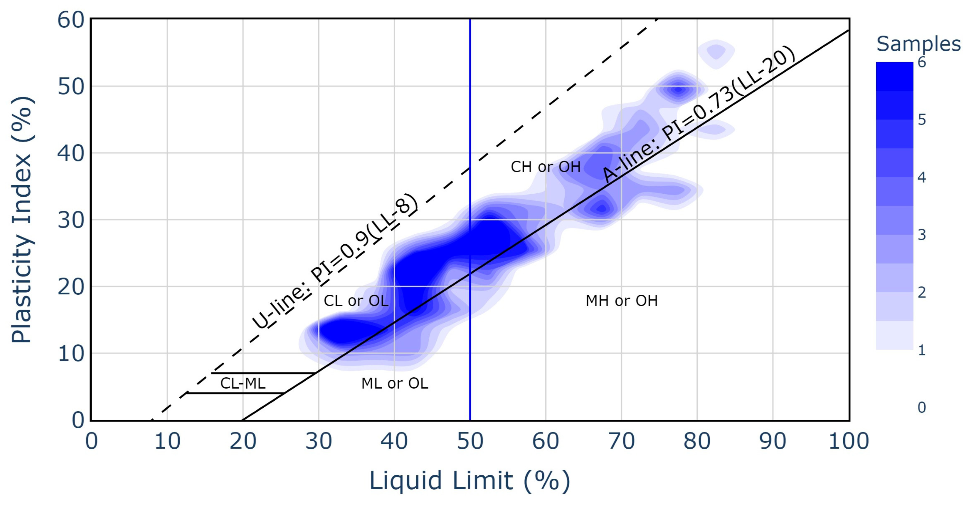
Next, all soils were classified according to the USCS. The results of this classification are presented in

Table 2. Distribution of soil samples according to the Unified Soil Classification System (USCS).

SUCS	CL	CH	ML	MH
Samples	73	70	15	23

. In addition, Figure 4 presents the distribution of the 181 undisturbed soil samples on the Casagrande plasticity chart, with colour intensity representing sample density. Most samples are concentrated above the A-line, corresponding predominantly to clays of medium to high plasticity (CL and CH, according to the USCS). A dense cluster can be observed between LL values of 30 and 60% and PI values of 12–32%, indicating a dominance of plastic clayey soils. Only a few samples (approximately 20%) fall below the A-line, within the silt categories (ML or MH). Specifically, the results of this classification indicate that 143 samples correspond to clays (C), 48 to silts (M), 93 to high-plasticity soils (H) (LL ≥ 50), and 50 to low-plasticity soils (L) (LL < 50). Moreover, according to Chen’s [45] criteria, 102 of these samples would be classified as moderately expansive and 51 as highly expansive.

In summary, the dataset covers a wide range of geotechnical conditions representative of expansive soils in southeastern Spain. According to their index properties, the soils span low- to high-plasticity ranges and include both clays and silts, as confirmed by the subsequent USCS classification. This variety of properties supports the generalizability and robustness of the proposed models.

Next, p-values and Variance Inflation Factor (VIF) for the predictive variables were calculated (

Table 3. VIF and p-values for the predictive variables.

Variable	Pass #0.075	LL	PI	w	γd
p-value	2.91 × 10−12	2.04 × 10−8	1.76 × 10−60	8.52 × 10−1	4.30 × 10−4
VIF	31.91	52.71	26.65	25.51	15.04

). The p-value represents the probability that the observed relationships between the independent variables and the dependent variable occurred by chance. A lower p-value indicates a statistically significant effect, typically below a threshold of 0.05. VIF measures multicollinearity among independent variables, with values above 10 suggesting a high degree of correlation. In the analysis, the p-values for the percentage of soil passing #0.075 mm, LL, PI, and γ_d were well below 0.05, indicating that these variables had a statistically significant impact on the dependent variable. Conversely, w presented a high p-value (0.852), suggesting it is not significantly contributing to the model. The VIF values indicated strong multicollinearity, particularly for LL and the percentage of soil passing #0.075 mm, as these properties are related to most of the others.

Additionally, the correlation matrix between the variables of the dataset is presented in Figure 5, using the Pearson correlation coefficient (r) and the Spearman coefficient. These correlation matrices revealed critical insights about the relationships between soil properties and p_s. Pearson correlations indicate linear dependencies, while Spearman correlations capture monotonic relationships, providing a comprehensive view of variable interactions.

For the target variable (p_s), both matrices showed consistently strong associations, though with notable differences in magnitude. PI exhibited the highest correlation with p_s in both methods, suggesting PI is the most reliable predictor. LL also showed strong positive correlations, reinforcing its importance in swelling prediction models. Water content demonstrated moderate correlations, indicating a secondary role in swelling behaviour, as well as showing a moderate to high correlation with the percentage of soil passing #0.075 mm and a very high p-value. γ_d showed a weak negative correlation with p_s, which may justify its inclusion as a secondary predictor, especially considering its low correlation with the other variables. The percentage of soil passing #0.075 mm presented moderate positive correlations, though the Spearman coefficient is notably lower, suggesting the relationship may involve nonlinear components.

5. Methodology

This section details the methodological framework adopted in the study, encompassing SR algorithms and sensitivity analysis techniques.

5.1. Deep Symbolic Regression

Petersen et al. [46] introduced a deep symbolic regression framework using reinforcement learning (RL) to recover symbolic functions in noisy environments. Building on this, Tenachi et al. [47] developed the Physical Symbolic Optimization (PhySO) framework, which combines deep RL and recurrent neural networks (RNNs) to derive analytical symbolic expressions from physical data while maintaining unit consistency. PhySO can use dimensional analysis to narrow the search space, ensuring that generated expressions align with physical principles.

Unlike conventional SR methods [27], which disregard physical units, PhySO ensures dimensional homogeneity by imposing constraints during equation generation. The PhySO process begins with data acquisition, followed by candidate symbolic expression generation using RL and RNNs. These expressions are structured as binary trees, with each node representing predefined elements, tokens, such as variables, operators, and constants. PhySO encodes these elements as categorical tokens and formulates expressions in prefix notation.

To optimize the search, PhySO evaluates symbolic expressions through a reinforcement learning approach, assigning rewards based on equation accuracy and unit consistency. The reward function balances accuracy (measured by Normalized Root Mean Square Error (NRMSE)) and simplicity, promoting models that are both precise and simple, avoiding overfitting. PhySO’s strategy uses a risk-seeking policy and entropy regularization, reinforced by the Adam optimizer. The network architecture relies on Long Short-Term Memory (LSTM) networks, which process input data sequentially and adjust probability distributions over actions. A masking mechanism filters invalid operations to ensure unit consistency.

5.2. High-Performance Symbolic Regression

High-performance symbolic regression (PySR) [48] is an evolutionary algorithm designed to search for mathematical expressions that best fit a dataset. PySR explores a large space of potential equations to uncover interpretable relationships, following an evolve–simplify–optimize loop that refines candidate equations by optimizing unknown scalar constants. PySR uses a tournament-style evolutionary algorithm with selection, crossover, and mutation processes to evolve expressions represented as tree structures. It employs a multi-population strategy, where separate populations evolve in parallel, occasionally exchanging candidate expressions to enhance diversity. The “hall of fame” stores the best solutions, serving as a reference for future generations. The algorithm utilizes regularized evolution [49,50], simulating natural selection to breed new expressions by subsampling the fittest candidates. The score metric evaluates trade-offs between accuracy gain and complexity. A key feature of PySR is explicit constant optimization using the Broyden–Fletcher–Goldfarb–Shanno algorithm, enabling fine-tuning of numerical parameters. An adaptive complexity penalty prevents overfitting, favouring simpler models when accuracy differences are negligible. PySR balances predictive performance with interpretability by using mean square error (MSE) and complexity metrics. It visualizes the trade-off between accuracy and complexity through Pareto fronts, ensuring models remain interpretable and effective across various fields, such as physics, engineering, and data-driven scientific discovery.

5.3. Multi-Objective Symbolic Regression

Multi-objective symbolic regression (MOSR) enhances traditional SR by optimizing multiple criteria simultaneously, rather than just focusing on prediction error. This approach addresses the issue of overly complex expressions that may not generalize well, offering a better balance between accuracy, simplicity, and interpretability. This work used a MOSR algorithm [51,52] built upon the Non-dominated Sorting Genetic Algorithm II (NSGA-II) [53], an selective multi-objective genetic algorithm where program ranking is based on non-dominance criteria and crowding distance metrics. Unlike single-objective approaches, which prioritize a single metric such as prediction accuracy, MOSR optimizes for both prediction accuracy and complexity simultaneously, ensuring that the resulting expressions are both accurate and interpretable. The algorithm sorts solutions based on Pareto optimality, where non-dominated solutions are assigned to the first Pareto front and subsequent fronts are populated with solutions that are less optimal but still offer useful trade-offs. The crowding distance metric promotes diversity in the population, encouraging a more thorough exploration of the solution space. To handle constants within expressions, the algorithm includes a local optimization procedure. This process uses a single-neuron neural network where the expression itself acts as the activation function, and constants are optimized using the Adam optimizer [54] with a binary cross-entropy loss function. This integration of genetic programming with gradient-based optimization enhances the search for more accurate and interpretable mathematical expressions.

5.4. Physics-Guided Symbolic Regression

Physics-guided symbolic regression (PGSR) incorporates physical principles and domain knowledge to guide the search for mathematical expressions. AI Feynman 2.0 [55,56] exemplifies this approach by combining neural network fitting with physics-inspired techniques, such as dimensional consistency, low-order polynomial structure, and compositionality. The process begins with dimensional analysis, using the Buckingham π-theorem to convert input variables into dimensionless quantities, ensuring unit consistency. If this step does not work, the algorithm reverts to the original problem setup. Next, polynomial regression is applied to fit low-degree polynomials to the data, assuming many physical relationships follow such patterns. When polynomial fitting is insufficient, the algorithm performs a combinatorial search over a restricted set of mathematical operators and functions, prioritizing simple expressions based on dimensional homogeneity and smoothness. If needed, neural networks analyse residuals to identify latent properties such as symmetry or separability, breaking down complex functions into simpler components. The algorithm recursively applies the entire pipeline to these subproblems, ensuring dimensional consistency and smoothness at each stage.

5.5. Sobol Sensitivity Analysis Method

The Sobol method [57] is a global sensitivity analysis technique that quantifies the influence of each input variable and their interactions on a model’s output. Based on variance decomposition, it assigns indices that measure both individual (first-order) and combined (second-order and total) effects. First-order sensitivity indices (S1s) measure the effect of each variable individually, while keeping all other variables constant. Total-order sensitivity indices (STs) measure the total effect of each variable on the output, including both its individual effect and its interactions with other variables. In this way, higher-order effects can be obtained by calculating the difference between both indices (ST-S1). The Sobol method is particularly useful for nonlinear models or those with multiple parameters, as it provides a comprehensive understanding of the system’s behaviour. Widely used in scientific simulations and engineering, it helps identify the most influential variables and can assist in reducing model complexity.

5.6. Comparative Overview of the Symbolic Regression Techniques

The four SR methods employed in this study follow different paradigms, offering complementary strengths. PhySO relies on deep reinforcement learning with physical constraints, ensuring unit consistency and physically meaningful equations. PySR, in contrast, uses a high-performance evolutionary algorithm focused on accuracy–simplicity trade-offs, with explicit constant optimization. MOSR is a multi-objective genetic programming approach, optimizing simultaneously for accuracy and complexity while encouraging diverse solutions. PGSR integrates symbolic regression with physics-guided heuristics, such as dimensional analysis and low-degree polynomial fitting. While PhySO and PGSR prioritize physical consistency through embedded constraints or analytical strategies, PySR and MOSR focus more on evolutionary discovery and computational efficiency. This methodological diversity enables a robust evaluation of SR capabilities and allows for contrasting equation forms and variable sensitivities in the predictive models. To complement the comparative overview, Figure 6 provides a schematic representation of the core computational structure of each symbolic regression method discussed.

6. Results and Discussion

A consistent random seed was applied to divide the dataset into 70% for training and 30% for testing, ensuring reproducibility in the model evaluation. In engineering applications, it is often essential to maximize predictive accuracy while keeping the resulting expressions simple; however, these objectives can be at odds. To derive the final equations, each symbolic regression algorithm was trained through multiple iterations, progressively increasing the allowed complexity. In each case, a pool of candidate formulas was generated and assessed based on a trade-off between predictive performance and simplicity. To avoid overfitting and ensure model interpretability, complex or higher-order terms were penalized or excluded. The final expressions were chosen by comprehensively evaluating each candidate for both predictive performance and structural simplicity. The results of this process were the formulas included in

Table 4. Formulas obtained for each SR algorithm implemented.

SR Model	Equation
PhySO	${\mathrm{p}}_{\mathrm{s}}\left(\mathrm{k}\mathrm{P}\mathrm{a}\right)=0.070·(\mathrm{P}\mathrm{I}-0.150·\mathrm{L}\mathrm{L})·(\#0.075\mathrm{m}\mathrm{m}+\mathrm{P}\mathrm{I}+0.180)$	(1)
PySR	${\mathrm{p}}_{\mathrm{s}}\left(\mathrm{k}\mathrm{P}\mathrm{a}\right)={\displaystyle \frac{\mathrm{PI}·\left(\#0.075\mathrm{mm}\right)+{\mathrm{PI}}^2-2127.643}{{\mathsf{\gamma }}_{\mathrm{d}}}}-\mathrm{LL}+147.092$	(2)
MOSR	${\mathrm{p}}_{\mathrm{s}}\left(\mathrm{k}\mathrm{P}\mathrm{a}\right)={\displaystyle \frac{2 · \left(\#0.075\mathrm{mm}\right)·{\mathrm{PI}}^2}{\mathrm{LL}·{\mathsf{\gamma }}_{\mathrm{d}}}}$	(3)
PGSR	${\mathrm{p}}_{\mathrm{s}}\left(\mathrm{k}\mathrm{P}\mathrm{a}\right)={\displaystyle \frac{\mathrm{PI}·\left(\#0.075\mathrm{mm}+\mathrm{PI}-w\right)}{{\mathsf{\gamma }}_{\mathrm{d}}}}$	(4)

.

To ensure reproducibility, the main hyperparameters adopted for each model were included in

Table A1. Hyperparameters adopted in the PhySO model.

Parameter	Fixed Constants	Free Constants	Units	Parallel_Mode	Reward_Function	Epochs	Batch-Size	n_Steps
Adopted value	0	2	without	False	SquashedNRMSE	100	10	20

,

Table A2. Hyperparameters adopted in the PySR model.

Parameter	Populations	Population_Size	Niterations	Maxsize	Model_Selection	Parsimony
Adopted value	50	28	400	15	“best”	0.01

,

Table A3. Hyperparameters adopted in the MOOSR model.

Parameter	Constants_Optimization	Optimization Task	WMSE Convergence Threshold	Population_Size	Tournament_Size	Generations_to_Train	Parsimony	Parsimony_Decay	Genetic_Operators_Frequency
Adopted value	scipy	regression:wmse	0.02	100	4	100	0.9	0.85	default except delete_node = 3

and

Table A4. Hyperparameters adopted in the PGSR model.

Parameter	polyfit_deg	BF_try_time	NN_epochs
Adopted value	1	70	200

. Hyperparameters not listed were those set by default in each model and therefore not modified. As much as possible, all algorithms were restricted to the use of basic operators: addition, subtraction, multiplication, division, exponentiation, square root, and logarithm, excluding more complex ones.

For the application of these equations, it is important to consider the input units, which are LL, PI, w, and #0.075 mm in % and γ_d in kN/m³, yielding p_s in kPa. Additionally, the ranges in which the algorithms were trained must be taken into account, as predictions outside these ranges may be unrealistic. The following are the ranges:

• Pass #0.075 mm (%): ≥28.2 and ≤100.0.
• LL (%): ≥27.7 and ≤85.1.
• PI (%): ≥7.9 and ≤57.8.
• w (%): ≥8.9 and ≤49.1.
• γ_d (kN/m³): ≥13.0 and ≤19.2.
• p_s (kPa): ≥17.2 and ≤514.2.

The parameters selected by each SR algorithm were different, except for PySR and MOSR, which selected the same parameters (all except w). This provides an advantage, as it enables the use of the equations depending on the available parameters. Natural water content was included in only one of the four equations (PGSR), in line with the findings of the statistical analysis conducted previously. It is normal not to observe a clear impact due to the undisturbed nature of the samples, as each sample has varying levels of water content and saturation.

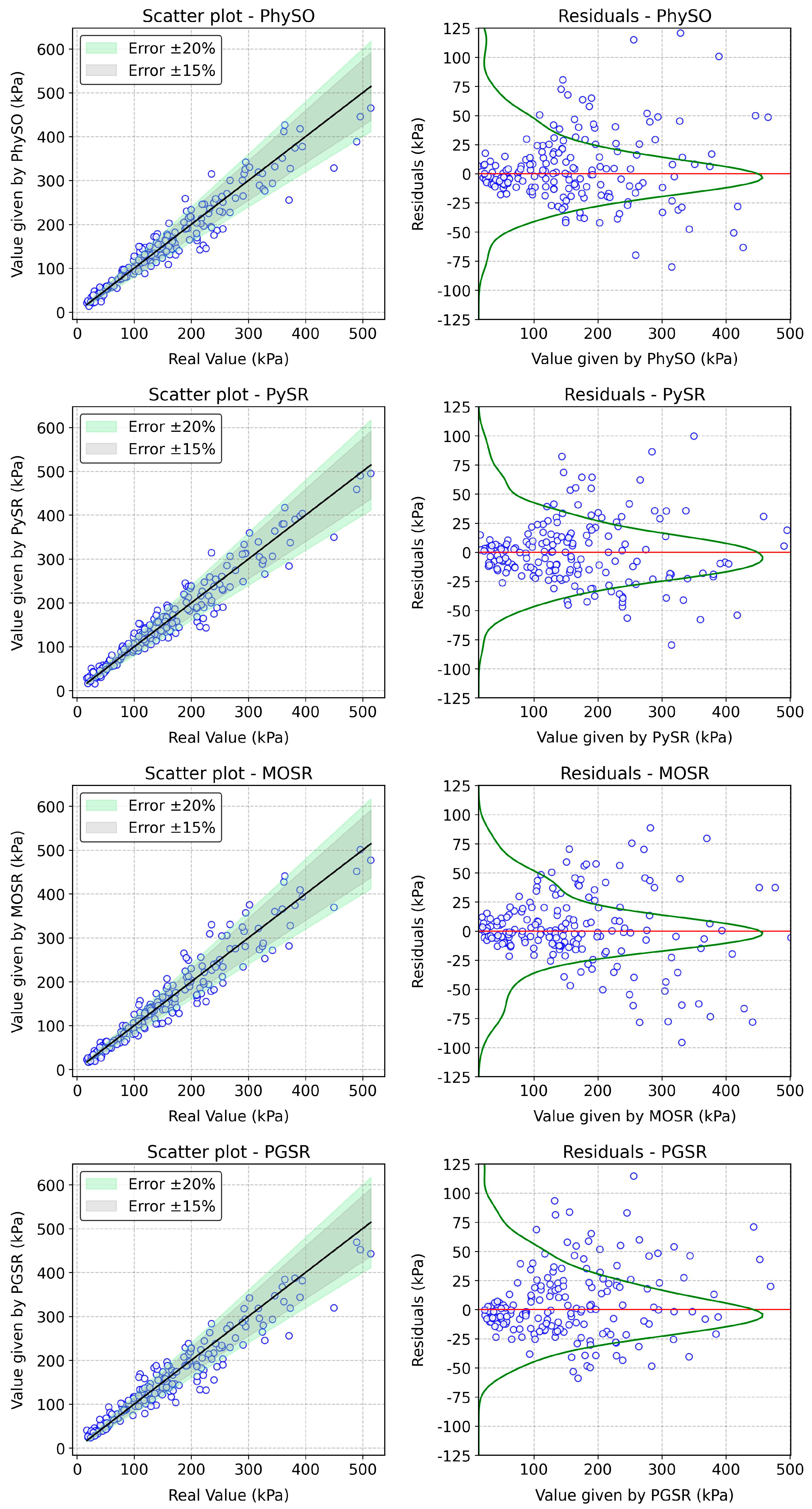
Figure 7 presents scatterplots illustrating the relationship between the actual values of p_s (x-axis) and the predicted values of p_s (y-axis) for the four SR algorithms considered. The analysis demonstrated that a significant portion of the data points lay in close proximity to the identity line and were mostly located within the error range of ±15%, indicating a strong agreement between the predicted and actual values. This suggests that the models performed well in accurately predicting p_s, with minimal deviation from the true values. The residuals (defined as the difference between the real and predicted values) are also shown in Figure 6, revealing that PhySO, MOSR, and PGSR slightly underestimated the predictions (mean residuals +3.20, +1.2, and +5.64 kPa, respectively), while PySR demonstrated near-zero bias (−0.16 kPa). PySR also exhibited the lowest standard deviation (STD) among the models (27.34 kPa), whereas PGSR showed the highest dispersion (STD = 30.94 kPa). Considering this global analysis, PySR emerged as the most robust model, exhibiting minimal bias and the lowest variability in residuals.

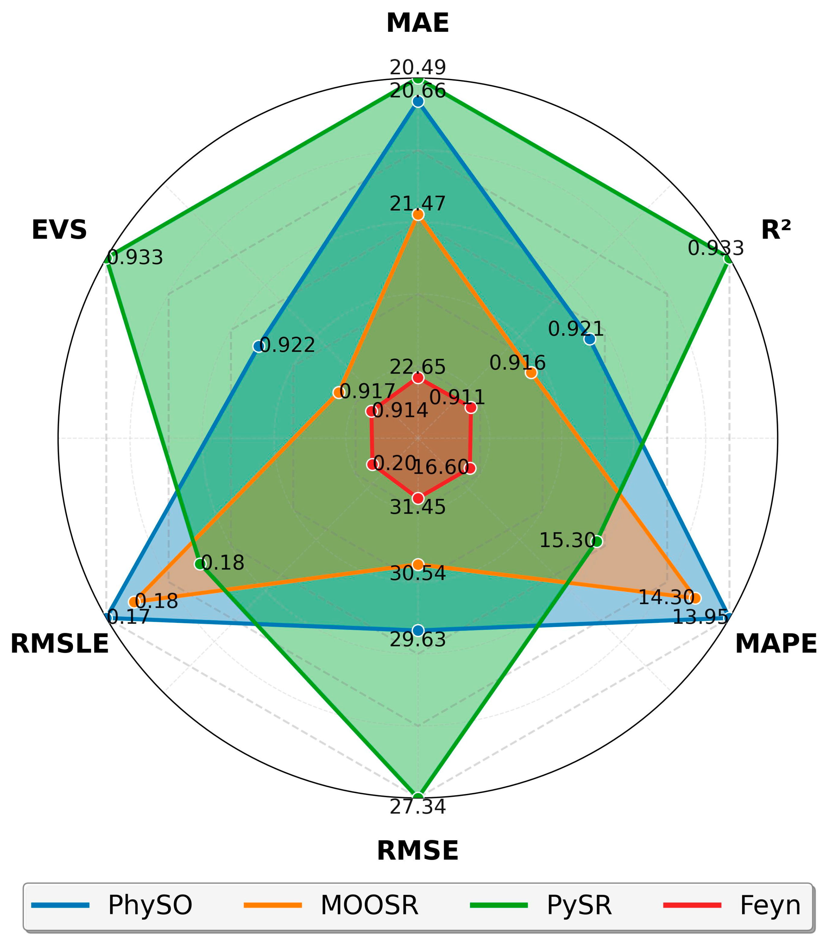
Based on the same residual and prediction data shown in Figure 7, a comparative summary of model performance was constructed using standard evaluation metrics, as shown in Figure 8. The evaluated metrics included Mean Absolute Error (MAE), Coefficient of Determination (R²), Mean Absolute Percentage Error (MAPE), Root Mean Square Error (RMSE), Root Mean Square Logarithmic Error (RMSLE), and Explained Variance (EVS). The results of this analysis are included in Figure 8 as a radar chart. The performance analysis of the four models revealed differences across the considered metrics. PySR exhibited superior accuracy, with the lowest MAE (20.49 kPa) and RMSE (27.34 kPa), alongside the highest R² (0.933) and EVS (0.933), indicating a strong ability to capture data variability. PhySO, with an MAE of 20.66 kPa and RMSE of 29.63 kPa, performed competitively and achieved the lowest MAPE (13.95%) and a low RMSLE (0.174), making it particularly reliable in terms of relative errors. PhySO prioritized relative accuracy and performance across different data scales, while PySR optimized overall accuracy more effectively and demonstrated greater robustness against outliers. MOOSR displayed intermediate results, with an MAE of 21.47 kPa and RMSE of 30.54 kPa, and lower R² (0.916) and EVS (0.917), indicating that it explained less variance compared to PySR and PhySO. The PGSR model registered the highest error levels, MAE (22.65 kPa), RMSE (31.45 kPa), MAPE (16.60%), and RMSLE (0.205), along with the lowest R² (0.911) and EVS (0.914), suggesting it was less effective in capturing data variability. In summary, while all models demonstrated reasonable predictive capabilities, PySR and PhySO led in accuracy and consistency, with MOOSR being moderately effective and PGSR performing in a less robust manner.

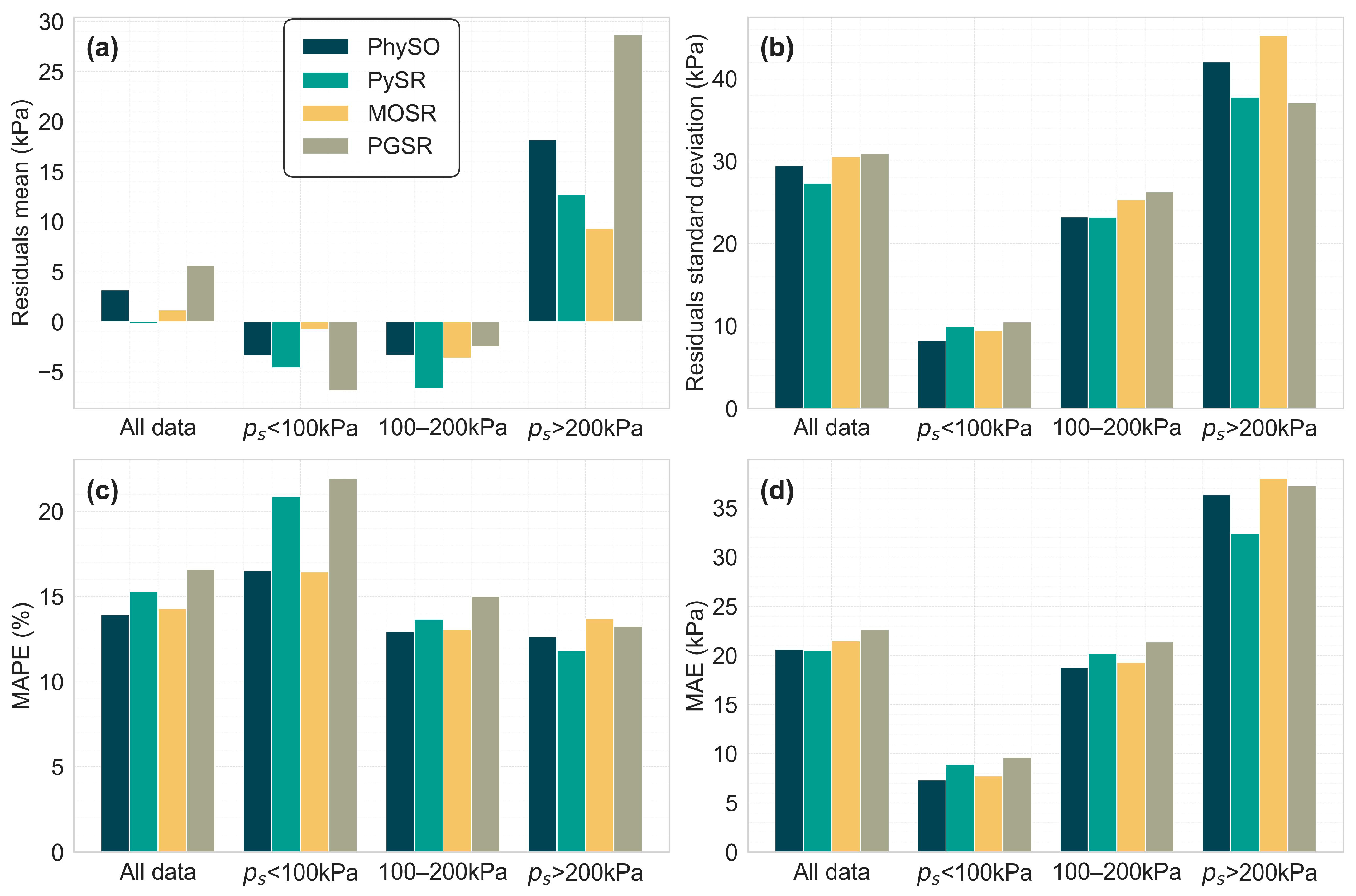
After completing the global analysis, a comparative analysis of the four SR regression models was conducted across different ranges of p_s. The dataset was then divided into several ranges of p_s: below 100 kPa, between 100 and 200 kPa, and above 200 kPa. For this analysis, MAPE, MAE, the mean, and the STD of the residuals were calculated. The results of this analysis are presented in Figure 9.

This analysis revealed distinct strengths for each model depending on the p_s interval. PhySO showed the best overall performance in relative terms, achieving the lowest MAPE on the full dataset and in the 100–200 kPa range (12.96%), and nearly the best in the <100 kPa segment. It also recorded the lowest residual STD in the <100 kPa range (8.27 kPa) and was close to the best in the 100–200 kPa range, indicating high precision at low to mid p_s. However, it exhibited notable bias in the extreme pressure ranges, particularly in >200 kPa (mean residuals = 18.20) and <100 kPa (−3.36 kPa), and its dispersion at high p_s (STD = 42.06 kPa) was among the highest. PySR minimized global bias most effectively (mean residuals = −0.16 kPa) and achieved the lowest MAPE (11.81%) and STD (37.79 kPa) in the ≥200 kPa range, making it particularly well-suited for high p_s applications. However, its performance in the <100 kPa range was not among the best, with the second highest MAPE (20.88%) and residual bias (−4.60 kPa). MOSR was the most robust in reducing residual bias at the extremes, with near-zero mean residuals in <100 kPa (−0.74 kPa) and the best bias in ≥200 kPa (9.36 kPa). Its MAPE in the low-pressure range (16.45%) was better than that of PhySO and PySR, although very close to PhySO. However, it exhibited high dispersion in the >200 kPa range (STD = 45.24 kPa) and demonstrated good performance in the 100–200 kPa range. PGSR demonstrated limited strengths compared to the other models. It showed moderate performance in the 100–200 kPa range but performed worst in terms of bias and MAPE in both the low (<100 kPa) and high (>200 kPa) ranges. Its lack of consistency made it the least competitive model overall, although its metrics remained good for the analysed case. In conclusion, PhySO was the most balanced model for general use, demonstrating strong performance particularly in low- to medium-pressure predictions. PySR excelled in high-pressure predictions while also maintaining good overall performance. MOSR minimized bias at the extremes and can be suitable for low to medium pressures, whereas PGSR did not exhibit a clear advantage in any specific pressure range. These strengths and weaknesses according to ranges should be considered along with the fact that each equation has parameters that others do not. Only PySR and MOSR share the same input variables (see Table 4), so depending on the available parameters and the intended objective, the most suitable equation can be selected.

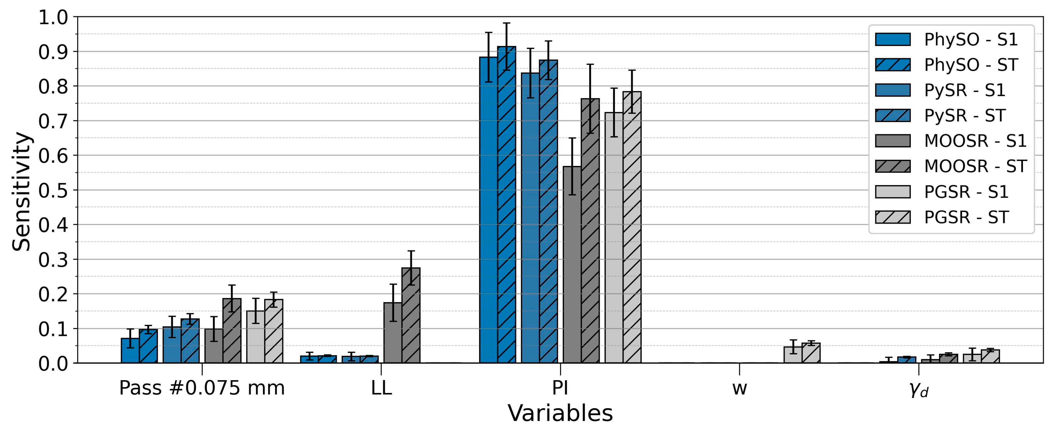
Next, a sensitivity analysis of the parameters involved in the four equations proposed was conducted. To this end, Sobol’s method [57] was applied. It is commonly used to evaluate the significance of input parameters in computational models with respect to their impact on the output based on the contribution to the output variance. Figure 10 presents the results of this analysis, including the S1 and ST values.

In all four models, PI was the dominant factor, with high S1 and ST indices. In PhySO and PySR, PI accounted for almost all of the variability (ST ≈ 0.91 and 0.87; S1 ≈ 0.88 and 0.84, respectively), while the percentage of soil passing #0.075 mm showed moderate contributions, and both LL and γ_d contributed very little. In MOOSR, PI remains crucial (ST ≈ 0.76; S1 ≈ 0.57), but the influence of LL increases (ST ≈ 0.27; S1 ≈ 0.17), suggesting that interactions, deduced from the difference between ST and S1, begin to play a greater role. In PGSR, in addition to the predominance of PI (ST ≈ 0.78; S1 ≈ 0.72), stronger interaction effects are observed, with noticeable contributions from w and γ_d (ST ≈ 0.057 and 0.037). While the individual effects of PI dominate across all models, interaction effects become more relevant in MOOSR and, to a lesser extent, in PGSR.

These findings align with the established knowledge in geotechnical engineering regarding expansive soil behaviour. PI, LL, and the percentage of soil passing #0.075 mm are identified as the most significant parameters in predicting swelling pressure. Their importance stems from their direct correlation with the mineralogical composition and plasticity characteristics that govern water adsorption capacity and expansive potential. Conversely, w exhibits a relatively lower influence on the predictive model. This phenomenon can be attributed to the use of undisturbed samples exhibiting varying degrees of initial saturation. Since the natural water content does not represent a controlled or comparable condition across different samples, its contribution to p_s prediction becomes less pronounced.

7. Conclusions

This study has demonstrated the potential of advanced techniques of SR in predicting p_s in clayey soils, a critical geotechnical property. The research has provided several key insights and contributions:

• Four advanced symbolic regression techniques (PhySO, PySR, MOSR, and PGSR) were applied, all showing strong predictive performance (R² > 0.91 and MAE < 23 kPa) along with highly simplified equations. PhySO and PySR outperformed the others in global metrics, with R² values of 0.921 and 0.933 and MAEs of 20.66 and 20.49 kPa, respectively. When analysing performance across pressure intervals, PhySO demonstrated the most balanced and robust behaviour, particularly excelling in low- to medium-pressure predictions. PySR achieved the highest accuracy under high-pressure conditions while maintaining consistent overall performance. MOSR stood out for its ability to reduce edge-case bias and was effective in low- to medium-pressure ranges, whereas PGSR showed no distinct advantage in any specific interval.
• Since each equation obtained from each model has different variables and performances across different pressure intervals, this allows for a quick determination of p_s based on the available parameters, the potential pressure range, and the objective of the analysis.
• This study identified PI as the most significant variable influencing p_s, surpassing the other variables in all models.
• A remarkable aspect of this study is the use of undisturbed clay samples. The undisturbed nature of these samples provides a more accurate representation of the natural conditions, enhancing the reliability and applicability of the findings.

The database used in this study could be further expanded with additional samples to improve the generalizability and scope of the proposed equations. As with any predictive algorithm, it is essential to consider that the model’s performance and the reliability of the expressions may decrease when applied outside the training range of the input variables.