Abstract
Cloud computing is widely used by organizations and individuals to outsource computation and data storage. With the growing adoption of machine learning as a service (MLaaS), machine learning models are being increasingly deployed on cloud platforms. However, operating MLaaS on the cloud raises significant privacy concerns, particularly regarding the leakage of sensitive personal data and proprietary machine learning models. This paper proposes a privacy-preserving decision tree (PPDT) framework that enables secure predictions on sensitive inputs through homomorphic matrix multiplication within a three-party setting involving a data holder, a model holder, and an outsourced server. Additionally, we introduce a leaf node pruning (LNP) algorithm designed to identify and retain the most informative leaf nodes during prediction with a decision tree. Experimental results show that our approach reduces prediction computation time by approximately 85% compared to conventional protocols, without compromising prediction accuracy. Furthermore, the LNP algorithm alone achieves up to a 50% reduction in computation time compared to approaches that do not employ pruning.
1. Introduction
It has been a long time since data was referred to as “the oil of the 21st century”. Today, many of the world’s most valuable companies thrive by collecting and monetizing vast amounts of data. However, such data often include sensitive personal information, making it inaccessible for public or collaborative use—not only due to commercial interests but also to mitigate privacy risks. Despite the significant potential of data sharing in addressing pressing societal challenges such as crime prevention, public health, and elder care, privacy concerns continue to severely limit the practical use of sensitive datasets across institutional boundaries. To address this challenge, privacy-preserving machine learning (PPML) has emerged as a key paradigm for enabling data-driven insights without compromising confidentiality.
One of the most prominent PPML frameworks is federated learning (FL) [1], which allows multiple parties to collaboratively train machine learning models without sharing their raw data. Each participant trains a local model and shares only model updates with a central server, preserving data privacy. However, FL assumes that participants have sufficient computational capacity for local training. In many real-world settings, particularly for devices or institutions with limited resources, local computation must be outsourced, raising new privacy concerns–even under semi-honest threat models.
This paper focuses on another type of PPML scenario in which a local entity securely outsources prediction computations. In our setting, both the data and the model remain encrypted, ensuring the confidentiality of sensitive user input and the intellectual property of the model provider. This setup is especially effective in protecting against model inversion attacks [2], which constitute a well-known vulnerability in machine learning-as-a-service (MLaaS) platforms. To implement secure outsourced prediction, we employ homomorphic encryption (HE) [3], particularly in its somewhat homomorphic variant, named somewhat homomorphic encryption (SHE) [4], which supports a limited number of encrypted additions and multiplications with significantly improved efficiency over fully homomorphic schemes. This enables practical encrypted inference in real-world scenarios. Among the various machine learning models, decision trees are particularly attractive for privacy-preserving inference due to their interpretability and low computational cost. As a result, a growing body of research has focused on designing cryptographic protocols for privacy-preserving decision tree (PPDT) inference that minimize both communication and computational overhead while preserving privacy.
1.1. Related Work
Existing PPDT protocols can be broadly classified based on the cryptographic primitives they employ.
- HE-based protocols:
- HE supports computation over encrypted data without requiring decryption. Akavia et al. [5] used low-degree polynomial approximations to support non-interactive inference with communication costs independent of tree depth. Frery et al. [6], Hao et al. [7], and Shin et al. [8] adopted the TFHE, BFV, and CKKS schemes, respectively, for efficient computation with low multiplicative depth. Cong et al. [9] reported ciphertext size comparisons and proposed homomorphic traversal algorithms across various commonly used HE schemes. Most existing HE-based PPDT protocols are designed for two-party settings, similar to the linear-function-based scheme proposed by Tai et al. [10].
- Protocols based on other cryptographic primitives:
- Zheng et al. [11] employed additive secret sharing in a two-server setting, ensuring that no single party gained access to both the model and the data, while maintaining low communication overhead. MPC-based approaches, such as those reported b Wu et al. [12], combine additive HE with oblivious transfer (OT), offering strong privacy guarantees but often suffering from scalability issues, particularly with deep trees. Differential privacy (DP), although more commonly used during training [13], can complement cryptographic inference methods by adding noise to outputs to mask sensitive patterns. However, DP typically compromises utility and operates orthogonally to encrypted inference techniques.
Within this landscape, several notable HE-based PPDT approaches stand out. Tai et al. [10] proposed a prediction protocol using linear functions and DGK-based integer comparison [14], reducing complexity at the cost of requiring bitwise encryption. Lu et al. [15] enhanced efficiency via the XCMP protocol, based on Ring-LWE SHE, although it struggled with large input bit lengths and unstable ciphertexts. Saha and Koshiba [16] addressed this with SK17, encoding integer bits as polynomial coefficients to support larger comparisons. Wang et al. [17] further improved SK17 by introducing a faster comparison protocol and a non-interactive variant with reduced ciphertext functionality.
Despite these advancements, existing protocols still face challenges in simultaneously achieving high efficiency, scalability, low communication overhead, and full tree structure confidentiality—especially under realistic semi-honest adversary models.
1.2. Our Contributions
To overcome the above-mentioned limitations, we propose a novel three-party PPDT inference protocol that achieves secure, structure-hiding, and communication-efficient decision tree predictions over encrypted data and models. The key innovations of our work are as follows:
- Homomorphic matrix multiplication-based inference: Departing from polynomial approximation and linear path evaluation methods [10], we introduce homomorphic matrix multiplication as the primary operation for encrypted path computation. This novel application supports structured and scalable evaluation of encrypted inputs.
- Leaf node pruning during inference: We propose leaf node pruning at inference time, a novel runtime optimization that reduces the number of nodes involved in computation, significantly improving performance. Unlike traditional model pruning during training, this technique operates during encrypted inference.
- Structure-hiding inference protocol: The decision tree structure—including internal nodes and branching conditions—is fully hidden from both the client and the server. By ensuring that all path computations are homomorphically encrypted, the protocol mitigates leakage risks present in prior PPDT methods.
- Semi-interactive three-party architecture: Our protocol requires only one round of interactive communication between the data holder (client) and the outsourced server. No interaction is required from the model holder during inference. This design enables low-latency, real-world deployment scenarios.
To achieve these properties, we adopt the efficient integer comparison protocol by Wang et al. [17] and the homomorphic matrix multiplication techniques from [18,19] for encrypted path evaluation. By integrating homomorphic matrix multiplication, inference-time leaf node pruning, and tree structure hiding into a semi-interactive three-party framework, our method enables efficient, secure, and practical decision tree inference in untrusted environments. We evaluated the proposed PPDT protocol on standard UCI datasets [20] to demonstrate its performance and practicality.
2. Preliminaries
In this section, we summarize the related approaches used in our proposal. In Section 2.1, we first review the concept of decision tree and the approach of decision tree classification via the linear function that was introduced by Tai et al. in [10], which was concerned with two kinds of secure computations—comparison at each node of tree and linear function calculation for prediction. We focus on how to improve the efficiency of the above two operations:
- Comparison: We use Wang et al.’s protocol [17] instead of the DGK approach [14] to improve the efficiency of secure comparison in each node.
- Prediction: We use secure inner product/matrix multiplication to replace linear function in order to outsource prediction while maintaining the tree model secret.
Therefore, we recall the secure comparison scheme proposed by Wang et al. [17] in Section 2.2 and the secure matrix multiplication introduced by Doung et al. [18] in Section 2.3. The two schemes are both constructed on the ring-LWE-based homomorphic encryption (see Appendix A for details). The notations in this paper are listed in Notations Section.
2.1. Existing Decision Tree Classification
2.1.1. Decision Tree
Figure 1 presents an example of a decision tree. The decision tree is a function that takes as input the feature vector and outputs the class to which X belongs. Generally, the feature vector space is ; however, in this paper, we denote it as because the input is the encrypted attribute data. This paper’s decision tree is a binary tree and consists of two types of nodes: decision nodes and leaf nodes. The decision node outputs a Boolean value where is the feature vector’s index, and is the threshold. A leaf node holds the output value . In a binary tree, there are m decision nodes and leaf nodes. For example, Figure 1 shows the case of , .
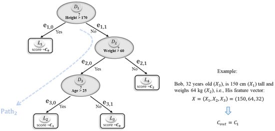
Figure 1.
Decision tree example.
2.1.2. Decision Tree Classification via Linear Function [10]
The Boolean output of the decision node , indicates that the next node is the left (right) child. For edges and , respectively connecting to the left child and the right child from the decision node , we define the corresponding edge cost as follows:
From the root node of the decision tree to each leaf node, only one path is determined. We define the path cost as the sum of the edge costs in —the path from root node to the leaf node . The edge cost and are determined by , which is the comparison result of decision node . Thereafter, the path cost for each leaf node is defined by a linear function of . For example, the following , and denote the path costs for leaf nodes , and in Figure 1, respectively:
The comparison results indicate that the edge cost to the next node is 0, while the edge cost to the other node is 1. As a result, only the path leading to a specific leaf node has a total cost ; all other paths have non-zero costs. The classification result is returned if and only if , meaning the output corresponds to the label stored in the leaf node .
This can be illustrated with a concrete example (see Bob in Figure 1): Bob’s attributes are height , weight , and age , which yield comparison results , , and , respectively. Substituting these into Equation (2), we compute the path costs as follows: , and only . Therefore, the output for Bob is , the label held by leaf node .
2.2. Secure Comparison Protocol
In this subsection, we describe the protocol proposed by Wang et al. [17], which securely computes the comparison of decision trees.
2.2.1. -bit Integer Comparison [14]
Assume that Alice and Bob respectively have two -bit integers, a and b, and consider how to compare two integers without revealing the values of a and b between Alice and Bob. Let us define the binary vectors for a and b as follows: and . In addition, let us define the following two binary vectors and where the first i-bits are the same as those in and while the remaining upper bits are set to zeros.
To compare the two integers a and b, let us define the following :
where
Here, is an inner product for calculating how many bits are different between and . Therefore, implies that the first i bits of a and b are the same (i.e., ). Next, we look at the -th bit of a and b when is satisfied. Here, could have the three values: 0, 1, or 2. If (i.e., ), ; otherwise, = 1 or 2. That is, if , is satisfied under ; otherwise, is satisfied. Therefore, to identify whether is satisfied, we merely need to check if in Equation (4) is 0 for any position of i ().
2.2.2. Packing Method
For a -bit length integer u whose binary vector is denoted as , the following packing polynomials are defined:
Using this packing method, we have [17]
where denotes the binary vector of the -bit integer , and and can be computed offline in advance. The coefficient of in is .
2.2.3. Secure Comparison Protocol
Wang et al. proposed three enhanced secure comparison protocols in [17]. Here, we recall the most efficient one that uses the packing method defined by Equation (6). There are three participants in this protocol. Alice and Bob who have -bit integers a and b, respectively, compare a and b without revealing the data through a server. The server obtains the comparison result, which is the output of the protocol. The protocol is described as follows:
- 1.
- Alice generates a secret–public key pair and sends to Bob and the server.
- 2.
- Alice and Bob computeandfor respectively, and send the results to the server.
- 3.
- The server computes
- 4.
- The server masks in encrypted form using random polynomialand sends to Alice.
- 5.
- Alice decryptsand sends back to the server.
- 6.
- The server unmasks d from as follows:and then verifies whether any -th term for is 0. If so ; otherwise, .
2.3. Ring-LWE-Based Secure Matrix Multiplication
Doung et al. proposed secure matrix multiplication [18] using the packing method proposed by Yasuda et al. [19]. For an ℓ-dimension vector , the following two polynomials are defined:
Note that for any two vectors and , using the above packing method, we have
where the constant term of provides the inner product .
Let be a (k, ℓ) matrix and let denote the row vectors of . For matrix , the packing method is defined as follows:
Assume that (n: dimension of polynomial ). Letting matrix be
and letting B denote an ℓ-dimensional vector, we have
where the coefficient of is , the inner product of vectors and B.
3. PPDT Classification Model
In this section, we propose a PPDT classification model that mainly consists of the following two processing parts:
(1) Path cost calculation and (2) secure integer comparison.
The basic idea of the path cost calculation comes from the Tai et al.’s decision tree classification protocol via linear function [10] where a decision tree model is treated as a plaintext under a two-party computation setting (see Section 2.1). In contrast, we extend the Tai et al.’s protocol such that not only input data but also a decision tree model can be encrypted to hide actual contents between a data provider and a model provider. To actualize this, we propose a secure three-party path cost calculation by extending the PPDT protocol proposed by Tai et al. [10] using the integer comparison protocol described in Section 2.2 that was proposed by Wang et al. [17].
3.1. Computation Model
To address the practical considerations of deploying our proposed algorithm in real-world cloud environments, we consider a scenario in which an organization that owns a decision tree classification model outsources the inference task by sending encrypted data to a cloud service provider (e.g., AWS and Google Cloud). Figure 2 illustrates the structure of our computational model, which involves three entities: the client, who possesses the feature vector to be classified; the model holder, who holds the trained decision tree; and the cloud server, which performs the encrypted computation on behalf of the model holder.
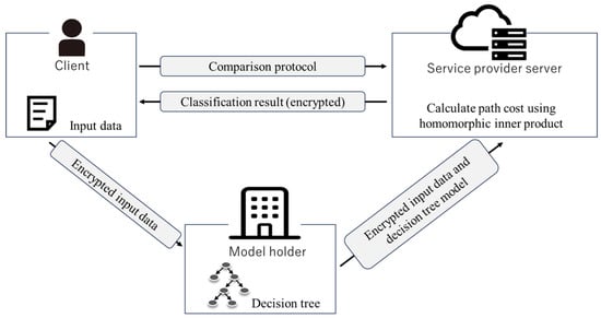
Figure 2.
Our computation model.
- The client encrypts the feature vectors and sends them to the model holder, who then encrypts the information needed to calculate the decision tree’s path cost and threshold.
- The client’s encrypted feature vectors are sent to the server, relaying the model holder, to conceal the information () about which elements of the feature vector threshold of the decision node should compare.
- On behalf of the model holder, the server performs the necessary calculation for the decision tree prediction and sends the client’s encrypted classification results.
- The client decrypts the information and obtains the classification results.
Even if the organization does not maintain its own servers, decision tree classification with privacy preservation is possible. The concrete process of the protocol is shown in Section 3.3.
A Representative Application of Online Medical Diagnostics
Machine-learned diagnostic models developed by medical institutions represent valuable intellectual property that is central to their competitive advantage. These institutions seek to offer diagnostic services without disclosing proprietary models, and cloud-based computation provides a practical solution to scale such services while reducing local computational costs.
However, concerns related to data confidentiality and model privacy present challenges for real-world deployment. Clients demand privacy-preserving services that do not expose their sensitive health data, while cloud service providers typically prefer not to manage or store sensitive information due to increased compliance and security risks.
Therefore, enabling secure and efficient inference over encrypted data and models aligns with the interests of all stakeholders. Our approach allows computations to be carried out on encrypted inputs and models, thereby mitigating privacy concerns and reducing the operational burdens associated with sensitive data management on cloud platforms.
3.2. Computation of Path Cost by Matrix × Vector Operation
In our method, we encrypt the path costs described in Section 2.1 and send them to the server to keep decision tree model secrets and allow the server to calculate the path costs. Specifically, we transform the path cost for a leaf node . Therefore, we introduce two vectors, and B, that can be used to calculate the path cost:
Here, B is a comparison result vector while is a path vector. We define path matrix of decision tree as follows:
Therefore, it is possible to replace the calculation of the path cost of the decision tree by . To obtain the correct multiplication result for a matrix and a vector of length ℓ using Equation (18), the constraint must be satisfied. Path matrix is an matrix; thus must be satisfied. Therefore, we divide the unconstrained path matrix into several rows and compute each of them. Specifically, is an matrix; thus, rows can be computed. The path matrix is divided into matrices. When , we add vector for several times so that each partitioned matrix has rows, which hides the size of the decision tree. With the above operations, we obtain S path matrices as follows:
Therefore, the secure matrix × vector operation in Section 2.3 allows us to securely compute the path cost with the encrypted path matrix.
3.3. Proposed Protocol
The protocol’s detailed procedure is illustrated in Figure 3 and Algorithm 1. It comprises eight steps involving data transmission and computation. Let K represent the number of classes in the classification task .
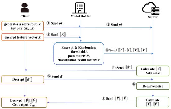
Figure 3.
Flowchart of the proposed protocol, where denotes the ciphertext of “·”.
The following provides a step-by-step description of the protocol:
- Step 1 (client):
- The client generates a secret–public key pair and sends to the model holder and server.
- Step 2 (client):
- The client encrypts each element of a feature vector by packing it using Equation (6).For , the client sends ciphertexts to the model holder.
- Step 3 (model holder):
- For , the model holder encrypts threshold by packing it using the Equation (6).For , the model holder generates path vector multiplied by a random numberand the following classification result vector is generated:where . As described in Section 3.2, the model holder generates S path matrices and S classification result matrices . Note that the path vector and classification result vector corresponding to the same path should be in the same matrix row.For , path matrix and classification result matrix are encrypted as follows:where Equation (16) is used to compute . A pair of ciphertexts of the elements of a threshold and its comparative feature vectorand ciphertext pairs of the path matrices and classification result matricesare sent to the server for and , respectively.
- Step 4 (server):
- The server calculates in Equation (10) as . The server masks in encrypted form using random polynomial and then sends to the client.
- Step 5 (client):
- The client decrypts and obtains , which is then returned to the server.
- Step 6 (server):
- The server obtains from Equation (13) and the comparison result vector . If any of the -th coefficients in is zero, then ; otherwise, .
- Step 7 (server):
- The server packs the comparison result vector B using Equation () to obtain . The server calculatesfor and sends to the client.
- Step 8 (client):
- The client obtains the number of path matrix using Equation (21), where . Then, for , it decrypts to obtain a polynomial with randomized non-zero coefficients for the path matrix , in which coefficients of are k-th path cost according to Equations (19) and (20). Since , then it is verified whether any -th term for is 0, which implies the corresponding path cost . If so, the corresponding leaf of is the classification result according to Equation (25), and the client decrypts and obtains from the coefficient of .
| Algorithm 1 Efficient PPDT Inference via Homomorphic Matrix Multiplication |
|
3.4. Leaf Node Pruning (LNP)
In this subsection, we describe how to reduce the number of path costs to be calculated. Let the number of leaf nodes of decision tree be and the number of classes to be classified be . In this case, we do not calculate the path cost for one class (e.g., ) but only the path cost for the other items. We compute the path cost corresponding to classes, and if any of them is 0, the output is the class corresponding to the path. If none of them is 0, the output is class corresponding to the uncalculated path. The detailed procedure is illustrated in Algorithm 3.
| Algorithm 2 Efficiency-Enhanced PPDT with LNP (Algorithm 1+LNP) |
|
Note that the default class must be securely shared in advance between the client and the model holder. Assigning the majority class as the default is generally more effective. The selection of the class excluded from computation depends on the classification task, as outlined below:
- Binary classification tasks
- (e.g., disease detection, abnormality detection): Only the decision path for class 1 (positive or anomalous) is evaluated. If the result is 0, class 1 is returned; otherwise, class 0 (negative or normal) is output.
- Multi-class classification tasks:
- Only classes are evaluated. If the dataset exhibits class imbalance (e.g., ImageNet), the majority class is assigned as the default. In the absence of such imbalance (e.g., MNIST), one class is randomly selected to serve as the default (i.e., the class not evaluated).
We next use a simple example to illustrate homomorphic matrix multiplication and the leaf node pruning process based on Figure 1 to enhance clarity and aid in reader understanding.
Example 1.
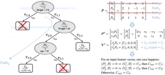
Figure 1 shows a decision tree example that is for three classes , in which the majority class is assigned as the default. Feature vector , where , and denote height, weight, and age, respectively. For example, client Bob, whose feature vector , tries to use the service to inference his health status. Decision tree has nodes with threshold . In this case, the comparison result vector can be expressed as .
From Figure 1, it can be easily seen that Bob’s data should be classified to leaf node by . In the following, we show how to perform classification inference using client Bob’s data and the model holder’s decision tree model while keeping them encrypted. According to Equations (2) and (19), we have
Therefore,
LNP process:
Pruning the leaf nodes with class , i.e., and , while multiplying by a random non-zero numbers , we obtain the path matrix
and the corresponding classification result matrix
Instead of using the original matrices P and V, we only need to use the pruned matrices and for calculation, thus saving computational cost, as shown in Figure 4.
Figure 4.
Image for LNP.
The following two processes are run on encrypted statuses.
Comparison on each node:
To check whether at node , let μ denote the bit length of the two integers and , where . For ease of explanation, we use as an example, with a bit length of .
- Server runs homomorphic operation to obtain polynomials of the comparison result and then adds a random polynomial using Equation (10) over a polynomial ring , which implies , as follows.where .
- Bob decrypts and sends back to the server. After removing the random polynomial γ from , the server can obtain comparison results from by checking whether ∃ any coefficient of . If so , set ; otherwise, .For example, , which is the coefficient of , so . Similarly, ; therefore, .
Classification inference:
- Bob decrypts and obtains the polynomial corresponding to a -dimension path matrix and then checks its coefficients of terms. In this example, , so whether the coefficient of or is zero is checked.In fact,and since ,
- the coefficient of is zero , and
- the coefficient of is zero ,
which links to leaf nodes and , respectively.As shown in Equation (38), since the coefficient of in the first polynomial is zero, if and only if , which means X is classified to leaf node . Then, the coefficient of in the second polynomial is the classification result; that is, .
3.5. Complexity
The client encrypts each element of the feature vectors with two different packing methods for comparison protocols and sends them to the model holder. The model holder encrypts the threshold for each decision node for times. In addition, the path and classification result matrices are encrypted times, respectively. The model holder sends the pairs of threshold and feature vector elements and the pairs of path and classification result matrices to the server. Next, the server and client cooperate to perform the comparison protocol for m times. In this case, the client performs decryption m times. The server performs homomorphic multiplication of the path and classification result matrices times and sends the client results. The client obtains the classification result by decrypting the received path and classification result matrices times.
3.6. Security Analysis
For a homomorphic encryption scheme, indistinguishability under chosen-plaintext attack (IND-CPA) is the basic security requirement. The SHE scheme used in the experiments in Section 4 is proven IND-CPA secure under the Ring-LWE assumption. In our proposed approach, as the input of the homomorphic computation consists of ciphertexts, the corresponding IND-CPA-secure SHE schemes will not be weakened.
Consider the entities involved in the protocol one by one (see Figure 3) and assume that they are all honest but curious and that they do not collude with one another.
- Client. The client can decrypt the ciphertext sent from the cloud server in Steps 5 and 7 using the secret key and obtain related to the comparison result and the decision tree structure. However, in Step 4, the noise from the cloud server is added for randomization. Therefore, the client receives a polynomial with completely random coefficients in . Similarly, is also a polynomial with random coefficients except zero, which leads to the classification ; that is, the coefficient corresponding to . Thus, the client can obtain the classification without knowing the decision tree model
- Model holder. The model holder only obtains the ciphertext of data X in Step 2, and IND-CPA security guarantees the privacy and security of the data.
- Cloud server. The server honestly performs homomorphic operations for the system but is curious about the data provided by the client and the model holder. In Step 3, it receives only encrypted inputs using an SHE scheme that satisfies IND-CPA security, ensuring the confidentiality of both user data and model parameters. Even if the server obtains the comparison result vector from d sent in Step 5, it cannot recover the original data X nor infer meaningful information about the decision tree (threshold t, path matrix P, and classification result V). This is due not only to encryption but also to randomization of P using noise terms and in Step 3, which prevents linkage to specific nodes of .
Beyond technical guarantees, our approach also addresses ethical challenges inherent to PPML in cloud environments. Specifically, it supports secure inference while protecting sensitive user data, ensuring model confidentiality and the reducing risks of unauthorized access or data misuse. These safeguards are especially crucial in sensitive domains such as healthcare and finance, where balancing performance with privacy and intellectual property protection is key to responsible AI deployment.
4. Experiments
4.1. Experimental Setup
We implemented the proposed PPDT protocol in C++ where the BFV method [21] in SEAL 3.3 [22] was used as the encryption library. In our implementation, the two comparison protocols were adopted: Wang et al.’s efficiency-enhanced scheme (Protocol-1 in [17]) and Lu et al.’s non-interactive private comparison (XCMP) [15]. The path cost calculation in Section 3.2 was implemented.
Parameter Choice. First, to ensure that the above comparison methods can accurately decrypt the comparison results, the parameters , and of the two methods must respectively satisfy the following two inequality requirements. Second, they must be selected to meet the 128-bit security level. The following parameters were used to ensure that the proposed model worked accurately and had 128-bit security, which is the currently recommended security level in [23]:
- Efficiency-enhanced scheme [17]These satisfy the following inequality: .
- XCMP [15]8192, 8191,These satisfy the following inequality: .
Note that is the default noise standard deviation used in Microsoft SEAL. The inequalities involving , and ensure the correctness of the corresponding comparison schemes. To support a maximum input bit length of ℓ, we chose n to satisfy the conditions from Wang et al. [17] (i.e., ) and Lu et al. [15] (i.e., ). Based on these constraints, the comparison protocols could handle 32-bit and 13-bit integers for Wang et al.’s and Lu et al.’s schemes, respectively. This implies that the efficiency-enhanced scheme [17] supports comparisons of larger integers than does XCMP [15], even with a relatively smaller n. Given the selected n, we chose q to ensure a 128-bit security level as recommended in [23] and then determined p such that it satisfied the necessary inequalities while remaining efficient to compute.
The experiments were conducted on a standard PC with the Core i7-7700K (4.20 GHz) processor using a single thread mode. We used scikit-learn, a standard open-source machine learning library in Python 3.7.2, to train the decision trees. In both the BFV method and the comparison protocol by Lu et al. [15], an input value must be represented as an integer . At every an appropriate number of times when the multiplication is performed, the fractional part of a value must be truncated, and it should be normalized within the range of .
In the performance evaluations, the computational time was measured by averaging over 10 trials for the following 8 data sets from the UCI machine learning repository [20]: Heart Disease(HD), Spambase (SP) (which were used for the benchmark in [15]), Breast Cancer Wisconsin (BC), Nursery (NS), Credit-Screening (CS), Shuttle (ST), EGG EYE State (EGG), and Bank Marketing (BK). The data set information and the parameters of the decision tree used are listed in Table 1.

Table 1.
Data set information and the size of trained decision tree.
4.2. Performance Comparisons
4.2.1. Path Cost Calculation
We compared the computational time to obtain the path costs under the three-party protocol when the proposed matrix multiplication in Section 3.2 and the Yasuda et al.’s homomorphic inner product calculation [19] were used. Table 2 shows the computational time for the path costs. We also show the computation time in parentheses when LNP was introduced into the proposed path cost calculation.
Table 2.
Computation time for path cost calculation in two methods: matrix multiplication of Section 3.2 and the homomorphic inner product calculation of Yasuda et al. [19] that we proposed in [24]. The computation time for the matrix multiplication with the addition of LNP is provided in parentheses. The computation time for LNP was measured as an average of 10 trials for each dataset class.
In calculating path costs by using the naive inner product, homomorphic multiplications are required. Therefore, as the number of nodes in a tree m increases, the computation time for path costs also increases. On the other hand, when calculating the path cost by matrix multiplication, for the decision tree of of Table 2, the path cost computation time was the same. The reason is that for parameter n, the entire path cost can be calculated with one matrix in the case of . Therefore, for datasets other than BK, more than one path cost can be computed with one matrix. The computation time for the path cost was reduced by more than 90% compared to the inner product case. However, in the case of BK, only path cost could be calculated with a single matrix multiplication. Hence, there is no difference in the computation time for matrix multiplication and inner product when .
With LNP being applied, the path cost computation time remained unchanged for decision trees (e.g., BC, ST, CS, HD) with , as all path costs could be computed within a single matrix. However, for larger trees (e.g., NS, SP, EGG, BK), LNP significantly reduced the computation time—by 26% for NS, 50% for SP, 48% for EGG, and 47% for BK. The effect correlated with the number of classes: datasets with fewer classes (SP, EGG, BK each with 2) benefited more than did NS (5 classes), as fewer classes enhance pruning efficiency. See Table 1 and Figure 5 for dataset-specific details.
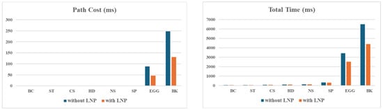
Figure 5.
Comparison of computation times with and without LNP across all datasets. For each dataset, the bar chart shows the path cost and total computation times, highlighting the reduction achieved by applying LNP. Datasets with fewer classes (e.g., SP, EGG, BK) showed more significant improvements due to more efficient pruning.
4.2.2. Protocol Efficiency
In this experiment, we used the XCMP of Lu et al. [15] for comparisons. We implemented two protocols and measured their computation times.
- To evaluate the efficiency of different homomorphic encryption approaches, we also integrated the XCMP scheme into the comparison component of the three-party protocol described in Section 3.3. The path cost computation was performed following the procedure outlined in Steps 6–8 of Section 3.3.
- A naive two-party protocol using XCMP by Lu et al. computed the result of two-party comparison (see Appendix B). Then, we computed the path cost under encrypt conditions by additive homomorphism.
Table 3 provides the measurement results.
Table 3.
Computation time with XCMP [15] in the following scenarios: three-party with matrix multiplication and LNP; two-party with homomorphic addition of XCMP results for computing the path cost.
In the naive two-party protocol, the path cost calculation is performed only by homomorphic addition, so addition is required. Therefore, the path cost calculation accounted more than 80% of the total time. In contrast, when applied to the proposed protocol, the path cost calculation time was reduced to 0.5% of the total time. As a result, the time reduction is achieved by applying XCMP to the proposed protocol on the experiments’ dataset. In particular, the reduction rate was higher for the EGG and BK datasets with a large number of decision nodes.
4.3. Time Complexity
To verify the computational complexity in Section 3.5, we measured the computation time of the proposed protocol for a decision tree constructed with the number of m decision nodes fixed between [10, 1000] using the BK dataset.
Figure 6 provides the experimental results that demonstrated that the computation time was linear with the number of decision nodes. There were several points at which there was a rapid increase in the number of times the model holder’s encryption was performed, the number of times the client was compounded, and the number of times the server’s path cost was computed. As illustrated in Section 3.5, these computation times depend on , where . Thus, as m increases, the computation time increases rapidly.
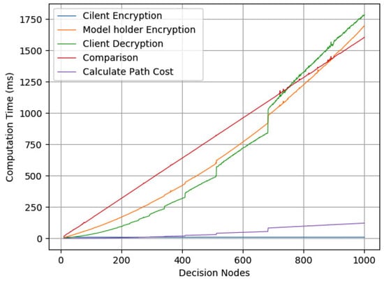
Figure 6.
Computation time for decision nodes.
5. Conclusions
In this paper, we proposed a privacy-preserving decision tree prediction protocol that enables secure outsourcing using homomorphic encryption. The proposed method uses the comparison protocol proposed by Wang et al. [17] or Lu et al. [15] to encrypt both feature vectors of a data holder and decision tree parameters of a model holder, and the structure of a decision tree model is hidden against both data holder and outsourced servers by calculating the path cost using the homomorphic matrix multiplication proposed by Dung et al. [18].
Our experimental results demonstrate that the computation time for three-party protocol using XCMP [15] is drastically reduced by more than 85% compared to the naive two-party protocol without a reduction in the prediction accuracy. In addition, we compared the method using homomorphic matrix multiplication [18] with homomorphic inner product [19]. As a result, we confirmed that there were cases where the computation time was reduced by more than 90%. We also proposed a leaf node pruning (LNP) algorithm to accelerate the three-party prediction protocol. The computation time was reduced by up to 50% when the proposed LNP was applied.
However, the proposed method has certain limitations. In particular, while the comparison results at each decision node are revealed to the outsourced server, the server cannot determine which specific feature each node corresponds to. This contrasts with the protocol by Lu et al. [15], which prevents such leakage but incurs significantly higher computational costs. This highlights a fundamental trade-off between security and computational efficiency: our approach enhances scalability and performance at the cost of limited information leakage. In many practical scenarios, this trade-off may be acceptable; however, minimizing data exposure remains a critical objective. In future work, we will aim to design a more efficient protocol that preserves performance while eliminating any information leakage, thereby strengthening both privacy and practicality.
Author Contributions
Conceptualization, S.F., L.W. and S.O.; methodology, S.F., L.W. and S.O.; software, S.F. and S.O.; validation, S.F. and S.O.; formal analysis, S.F. and L.W.; investigation, S.F. and L.W.; resources, S.O.; data curation, S.F.; writing—original draft preparation, S.F., L.W. and S.O.; writing—review and editing, L.W.; supervision, S.O.; project administration, S.O. and L.W.; funding acquisition, S.O. and L.W. All authors have read and agreed to the published version of the manuscript.
Funding
This work was partially supported by JST CREST (grant number JPMJCR21M1) and JST AIP accelerated program (grant number JPMJCR22U5), Japan.
Institutional Review Board Statement
Not applicable.
Informed Consent Statement
Not applicable.
Data Availability Statement
The original contributions presented in the study are included in the article; further inquiries can be directed to the corresponding author.
Acknowledgments
We would like to thank Takuya Hayashi for the useful discussion.
Conflicts of Interest
The authors declare no conflicts of interest.
Notations
The following notations are used in this manuscript:
| Functions that return 1 if · is true and 0 if false | |
| Maximum bit length of an integer | |
| A | Vector of length ℓ |
| d-bit subvector of A | |
| -bit binary vector of integer a, | |
| where is the least significant bit of integer a. | |
| N | Dimension of the feature vector |
| X | Feature vector |
| Decision node | |
| Leaf node | |
| Index of feature vectors to be compared by decision node | |
| Threshold of decision node | |
| Class to be output by leaf node | |
| m | Number of decision nodes in the decision tree |
| Number of leaf nodes in the decision tree |
Parameters being used in the ring-LWE-based encryption schemes:
| n | An integer of power of 2 that denotes the degree of polynomial . Define a polynomial ring , |
| q | An integer composed of ( is a prime number). Define a polynomial ring representing a ciphertext space , |
| p | Define a plaintext space , where p and q are mutually prime natural numbers with the relation , |
| Standard deviation of the discrete Gaussian distribution defining the secret key space . The elements of are polynomials on the ring . Each coefficient is independently sampled from the discrete Gaussian distribution of the variance . |
Appendix A. Ring-LWE-Based Homomorphic Encryption
This study used the ring-LWE-based public key homomorphic encryption library called the Simple Encrypted Arithmetic Library (SEAL) v.3.3 [22] to implement our protocols. SEAL implements the somewhat homomorphic encryption scheme proposed by Fan et al. [21]. Due to the additive and multiplicative homomorphism, packing plaintexts provides an efficient homomorphic inner product and matrix multiplication calculations. See [21,22] for details on the encryption scheme.
The somewhat homomorphic encryption scheme consists of the following four basic algorithms:
- : input security parameter and output system parameter .
- : input system parameter and output public key and secret key .
- : input plaintext m and output ciphertext c.
- : input ciphertext c and output plaintext m.
Homomorphic addition and multiplication algorithms are defined by and , and the corresponding decryption algorithms are represented by and , respectively. Let and denote the ciphertexts of the two plaintexts m and , respectively. Then, the sum and product of m and can be calculated as follows.
Hereafter, we write , and . The difference between c and can be obtained using homomorphic addition, and we define .
Appendix B. XCMP [15]
Assume that client and server have two ℓ-bit integer values such as a and b, respectively. According to the algorithm in Figure A1, the server computes to obtain the comparison result in encrypted form. In this scheme, the comparison result is a constant term in the polynomial C, as shown in . It is possible to perform scalar multiples, additions, and subtractions on the resulting ciphertext .
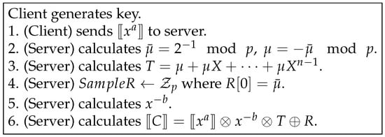
Figure A1.
XCMP [15].
References
- Konečný, J.; McMahan, H.B.; Ramage, D.; Richtárik, P. Federated Optimization: Distributed Machine Learning for On-Device Intelligence. arXiv 2016, arXiv:1610.02527. [Google Scholar] [CrossRef]
- Fredrikson, M.; Jha, S.; Ristenpart, T. Model Inversion Attacks that Exploit Confidence Information and Basic Countermeasures. In Proceedings of the 22nd ACM SIGSAC Conference on Computer and Communications Security, Denver, CO, USA, 12–16 October 2015; Ray, I., Li, N., Kruegel, C., Eds.; ACM: New York, NY, USA, 2015; pp. 1322–1333. [Google Scholar] [CrossRef]
- Rivest, R.L.; Dertouzos, M.L. On Data Banks and Privacy Homomorphisms. In Foundations of Secure Computation; DeMillo, R., Ed.; Academic Press: Cambridge, MA, USA, 1978; Volume 4, pp. 169–180. [Google Scholar]
- Gentry, C. A Fully Homomorphic Encryption Scheme. Ph.D. Thesis, Stanford University, Stanford, CA, USA, 2009. [Google Scholar]
- Akavia, A.; Leibovich, M.; Resheff, Y.S.; Ron, R.; Shahar, M.; Vald, M. Privacy-Preserving Decision Trees Training and Prediction. In Proceedings of the Machine Learning and Knowledge Discovery in Databases—European Conference, ECML PKDD 2020, Ghent, Belgium, 14–18 September 2020; Proceedings, Part I. Hutter, F., Kersting, K., Lijffijt, J., Valera, I., Eds.; Lecture Notes in Computer Science. Springer: Berlin/Heidelberg, Germany, 2020; Volume 12457, pp. 145–161. [Google Scholar] [CrossRef]
- Fréry, J.; Stoian, A.; Bredehoft, R.; Montero, L.; Kherfallah, C.; Chevallier-Mames, B.; Meyre, A. Privacy-Preserving Tree-Based Inference with TFHE. In Proceedings of the Mobile, Secure, and Programmable Networking—9th International Conference, MSPN 2023, Paris, France, 26–27 October 2023; Revised Selected Papers. Bouzefrane, S., Banerjee, S., Mourlin, F., Boumerdassi, S., Renault, É., Eds.; Lecture Notes in Computer Science. Springer: Berlin/Heidelberg, Germany, 2023; Volume 14482, pp. 139–156. [Google Scholar] [CrossRef]
- Hao, Y.; Qin, B.; Sun, Y. Privacy-Preserving Decision-Tree Evaluation with Low Complexity for Communication. Sensors 2023, 23, 2624. [Google Scholar] [CrossRef] [PubMed]
- Shin, H.; Choi, J.; Lee, D.; Kim, K.; Lee, Y. Fully Homomorphic Training and Inference on Binary Decision Tree and Random Forest. In Proceedings of the Computer Security—ESORICS 2024—29th European Symposium on Research in Computer Security, Bydgoszcz, Poland, 16–20 September 2024; Proceedings, Part III. García-Alfaro, J., Kozik, R., Choras, M., Katsikas, S.K., Eds.; Lecture Notes in Computer Science. Springer: Berlin/Heidelberg, Germany, 2024; Volume 14984, pp. 217–237. [Google Scholar] [CrossRef]
- Cong, K.; Das, D.; Park, J.; Pereira, H.V.L. SortingHat: Efficient Private Decision Tree Evaluation via Homomorphic Encryption and Transciphering. In Proceedings of the 2022 ACM SIGSAC Conference on Computer and Communications Security, CCS 2022, Los Angeles, CA, USA, 7–11 November 2022; Yin, H., Stavrou, A., Cremers, C., Shi, E., Eds.; ACM: New York, NY, USA, 2022; pp. 563–577. [Google Scholar] [CrossRef]
- Tai, R.K.H.; Ma, J.P.K.; Zhao, Y.; Chow, S.S.M. Privacy-Preserving Decision Trees Evaluation via Linear Functions. In Proceedings of the Computer Security—ESORICS 2017—22nd European Symposium on Research in Computer Security, Oslo, Norway, 11–15 September 2017; Proceedings, Part II. Foley, S.N., Gollmann, D., Snekkenes, E., Eds.; Lecture Notes in Computer Science. Springer: Berlin/Heidelberg, Germany, 2017; Volume 10493, pp. 494–512. [Google Scholar] [CrossRef]
- Zheng, Y.; Duan, H.; Wang, C.; Wang, R.; Nepal, S. Securely and Efficiently Outsourcing Decision Tree Inference. IEEE Trans. Dependable Secur. Comput. 2022, 19, 1841–1855. [Google Scholar] [CrossRef]
- Wu, D.J.; Feng, T.; Naehrig, M.; Lauter, K.E. Privately Evaluating Decision Trees and Random Forests. Proc. Priv. Enhancing Technol. 2016, 2016, 335–355. [Google Scholar] [CrossRef]
- Maddock, S.; Cormode, G.; Wang, T.; Maple, C.; Jha, S. Federated Boosted Decision Trees with Differential Privacy. In Proceedings of the 2022 ACM SIGSAC Conference on Computer and Communications Security, CCS 2022, Los Angeles, CA, USA, 7–11 November 2022; Yin, H., Stavrou, A., Cremers, C., Shi, E., Eds.; ACM: New York, NY, USA, 2022; pp. 2249–2263. [Google Scholar] [CrossRef]
- Damgård, I.; Geisler, M.; Krøigaard, M. A correction to ’efficient and secure comparison for on-line auctions’. Int. J. Appl. Cryptogr. 2009, 1, 323–324. [Google Scholar] [CrossRef]
- Lu, W.; Zhou, J.; Sakuma, J. Non-interactive and Output Expressive Private Comparison from Homomorphic Encryption. In Proceedings of the 2018 on Asia Conference on Computer and Communications Security, AsiaCCS 2018, Incheon, Republic of Korea, 4–8 June 2018; Kim, J., Ahn, G., Kim, S., Kim, Y., López, J., Kim, T., Eds.; ACM: New York, NY, USA, 2018; pp. 67–74. [Google Scholar] [CrossRef]
- Saha, T.K.; Koshiba, T. An Efficient Privacy-Preserving Comparison Protocol. In Proceedings of the Advances in Network-Based Information Systems, The 20th International Conference on Network-Based Information Systems, NBiS 2017, Ryerson University, Toronto, ON, Canada, 24–26 August 2017; Barolli, L., Enokido, T., Takizawa, M., Eds.; Lecture Notes in Computer Science; Springer: Berlin/Heidelberg, Germany, 2018; Volume 7, pp. 553–565. [Google Scholar] [CrossRef]
- Wang, L.; Saha, T.K.; Aono, Y.; Koshiba, T.; Moriai, S. Enhanced Secure Comparison Schemes Using Homomorphic Encryption. In Proceedings of the Advances in Networked-Based Information Systems—The 23rd International Conference on Network-Based Information Systems, NBiS 2020, Victoria, BC, Canada, 31 August–2 September 2020; Barolli, L., Li, K.F., Enokido, T., Takizawa, M., Eds.; Advances in Intelligent Systems and Computing. Springer: Berlin/Heidelberg, Germany, 2021; Volume 1264, pp. 211–224. [Google Scholar] [CrossRef]
- Duong, D.H.; Mishra, P.K.; Yasuda, M. Efficient Secure Matrix Multiplication Over LWE-Based Homomorphic Encryption. Tatra Mt. Math. Publ. 2016, 67, 69–83. [Google Scholar] [CrossRef]
- Yasuda, M.; Shimoyama, T.; Kogure, J.; Yokoyama, K.; Koshiba, T. Practical Packing Method in Somewhat Homomorphic Encryption. In Proceedings of the Data Privacy Management and Autonomous Spontaneous Security–8th International Workshop, DPM 2013, and 6th International Workshop, SETOP 2013, Revised Selected Papers, Egham, UK, 12–13 September 2013; García-Alfaro, J., Lioudakis, G.V., Cuppens-Boulahia, N., Foley, S.N., Fitzgerald, W.M., Eds.; Lecture Notes in Computer Science. Springer: Berlin/Heidelberg, Germany, 2014; Volume 8247, pp. 34–50. [Google Scholar] [CrossRef]
- Kelly, M.; Longjohn, R.; Nottingham, K. The UCI Machine Learning Repository. Available online: https://archive.ics.uci.edu (accessed on 31 March 2025).
- Fan, J.; Vercauteren, F. Somewhat Practical Fully Homomorphic Encryption. IACR Cryptology ePrint Archive 2012. p. 144. Available online: https://eprint.iacr.org/2012/144 (accessed on 31 March 2025).
- Microsoft SEAL (Release 3.3); Microsoft Research: Redmond, WA, USA, 2019; Available online: https://github.com/Microsoft/SEAL (accessed on 31 March 2025).
- Albrecht, M.; Chase, M.; Chen, H.; Ding, J.; Goldwasser, S.; Gorbunov, S.; Halevi, S.; Hoffstein, J.; Laine, K.; Lauter, K.; et al. Homomorphic Encryption Security Standard; Technical report; HomomorphicEncryption.org: Toronto, ON, Canada, 2018. [Google Scholar]
- Fukui, S.; Wang, L.; Hayashi, T.; Ozawa, S. Privacy-Preserving Decision Tree Classification Using Ring-LWE-Based Homomorphic Encryption. In Proceedings of the Computer Sequrity Symposium 2019, Nagasaki, Japan, 21–24 October 2019; pp. 321–327. [Google Scholar]
Disclaimer/Publisher’s Note: The statements, opinions and data contained in all publications are solely those of the individual author(s) and contributor(s) and not of MDPI and/or the editor(s). MDPI and/or the editor(s) disclaim responsibility for any injury to people or property resulting from any ideas, methods, instructions or products referred to in the content. |
© 2025 by the authors. Licensee MDPI, Basel, Switzerland. This article is an open access article distributed under the terms and conditions of the Creative Commons Attribution (CC BY) license (https://creativecommons.org/licenses/by/4.0/).