Research on Numerical Calculation Methods for Modelling the Dynamics of Diesel Engine Crankshaft System Substructures

Abstract

The complex structure of a diesel engine crankshaft, combined with diverse and dynamically changing loads, leads to the interaction of torsional, bending, and longitudinal vibrations. These complexities present challenges in achieving comprehensive and efficient dynamic modelling and analysis. This paper presents a dynamic modelling and numerical computation method for the crankshaft system based on the substructure dynamic model to address this. Specifically, the primary degrees of freedom (DOFs) of the crankshaft system are transformed through coupling between master and slave node DOFs and DOF condensation. A numerical method for free vibration analysis is developed using Cholesky decomposition and Jacobi iteration, while a dynamic response is computed based on the Newmark-β implicit integration algorithm. Additionally, an adaptive step-size control strategy based on the energy gradient criterion was proposed by introducing a dynamic relaxation factor, significantly enhancing computational efficiency. The study further examines the influence of primary DOF selection, coupling region size between master and finite element nodes, bearing support stiffness, and integration step size on the dynamic response. Numerical case studies demonstrate that the substructure model, with fewer DOFs, accurately characterizes the dynamic behaviour of the crankshaft by appropriately selecting primary DOFs and computational parameters, thereby enabling efficient dynamic analysis.

1. Introduction

As a core component of a diesel engine, the crankshaft system experiences continuous variations in output torque and crankpin load due to its structural characteristics and the constantly changing cylinder pressure. These variations induce coupled torsional, lateral, and longitudinal vibrations. If not properly controlled, such vibrations can result in excessive noise and significant mechanical stress, potentially damaging or failing the crankshaft and transmission system components [1]. Therefore, developing a dynamic model that accurately represents the characteristics of coupled vibrations is essential for analyzing crankshaft system vibrations and designing effective control strategies. With the ongoing advancement of diesel engines toward higher performance and higher reliability, research on this issue has received increasing attention.

Current methods for calculating the coupled vibration response of diesel engine crankshaft systems primarily include the finite element method, the spatial beam model method, and the substructure model method [2,3]. The finite element method provides high accuracy and strong versatility. However, its model construction is complex and highly sensitive to boundary conditions. Additionally, multi-cylinder diesel engine finite element models often contain a large number of degrees of freedom, resulting in significant computational demands for solving time-domain dynamic responses, making implementation challenging [4]. The spatial beam model method simplifies complex structures into beam elements, effectively reducing both the degrees of freedom and computational complexity, but its accuracy is limited. In contrast, when properly applied, the substructure model method significantly reduces the degrees of freedom and can accurately describe the dynamic behaviour of the crankshaft system, enabling precise time-domain calculations [5].

The substructure method was initially developed to solve large-scale static problems. Hurty [6] introduced the fixed-interface modal synthesis method, which decouples interface constraints. However, its application in large structural analysis remains overly complex. Craig and Bampton [7] refined this approach by constructing system modes using primary and constraint modes. Wang et al. [8,9] solved the nonlinear motion equations of coaxial rotor systems to determine their dynamic characteristics. Zhai et al. [10] developed a high-precision reduced-order model that decreases the degrees of freedom of linear components and reduces computational costs. Gao et al. [11] improved the interface modal method by establishing a reduced-order model for blade discs. Zheng et al. [12] proposed a reduced-order modelling approach for asymmetric rotors, which can be integrated with the interface modal synthesis method. Hou [13] pioneered the free-interface modal synthesis method, enabling independent modal analysis of substructures. Wang Tao et al. [14] enhanced this method by incorporating the perturbation approach for substructure analysis. Huang et al. [15] employed the Timoshenko beam model to develop a rotor-bearing coupled dynamic model and investigated the causes of abnormal resonance. Yu et al. [16] applied the substructure modal superelement synthesis method to analyze coupled vibrations in rotor systems, while Liu Ying et al. [17,18] introduced a parameterized reduced-order modelling approach based on substructures. Bai [19,20,21] advanced the substructure synthesis method to improve the efficiency and reliability of vibration characteristic calculations. Geradin [22] developed a node-free supplement formulation to enhance computational efficiency. Wu et al. [23] proposed a topology optimization method for substructure reduced-order models, enabling the explicit calculation of substructure-related density derivatives.

The substructure model method represents a developmental trend in calculating the dynamic response of complex structures, with an increasing number of software tools incorporating relevant computational functions [24]. However, challenges persist in creating crankshaft substructure models, the coupling relationships between master and auxiliary nodes, and the development of high-precision numerical methods for coupled vibration analysis. Therefore, this study uses the crankshaft of a six-cylinder diesel engine as a case study to explore establishing a substructure dynamic model and numerical solution methods while also examining the influence of various factors on the analysis results.

2. Crankshaft System Substructure Modelling

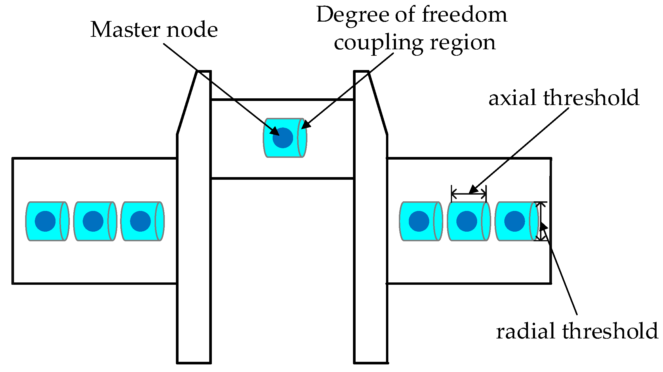
The six-cylinder diesel engine crankshaft is selected in this study due to its representative structural complexity and its widespread application in both marine and automotive diesel engines. The six-cylinder configuration provides a structurally balanced layout and exhibits typical vibration characteristics, making it an ideal platform for validating the effectiveness and applicability of the proposed modelling approach. The selection of master nodes and their degrees of freedom in the crankshaft substructure model must accurately represent crankshaft deformation, apply loads and constraints, and capture dynamic responses [25]. Using the crankshaft system of a six-cylinder diesel engine as an example, bearing constraints need to be defined at each main journal, assigning $m$ master nodes; loads need to be applied at the crankpins, also defining $n$ master nodes; an output torque need to be applied at the flywheel end, defining one master node; and the free end need to be connected to a damper, with its properties specified, also defining one master node. Typically, these numbers $m$ and $n$ are odd. Each master node contains six degrees of freedom, including three translational and three rotational components. A schematic diagram of the main nodes of the crankshaft substructure of the six-cylinder diesel engine is shown in Figure 1.

To reduce the degrees of freedom, the degrees of freedom of the finite element nodes must be condensed based on the established relationship between master nodes and finite element nodes. This process employs the Craig–Bampton fixed-interface modal synthesis method, combined with the dynamic substructuring approach based on double modal analysis proposed by Besset and Jezequel, to ensure the preservation of the structural physical characteristics during the degree-of-freedom condensation process [7]. Assuming that appropriate node numbering is applied, the stiffness matrix of the substructure, along with the corresponding nodal displacement and load vectors, can be expressed in a partitioned form as follows [26]:

$$\left[\begin{array}{cc}{K}_{bb}& K_{bi}\\ K_{ib}& K_{ii}\end{array}\right]\left(\begin{array}{c}{a}_b\\ a_i\end{array}\right)=\left(\begin{array}{c}{P}_b\\ P_i\end{array}\right)$$

(1)

where $a_b$ and $a_i$ represent the vectors of the crankshaft system’s master and finite element node degrees of freedom, respectively. The degrees of freedom of the internal nodes to be condensed within each substructure can be expressed as follows:

$$a_i=K_{ii}^{-1}\left(P_i-K_{ib}{a}_b\right)$$

(2)

Thus, the condensed equation is

$$K_{bb}^{\ast }{a}_b=P_b^{\ast }$$

(3)

where,

$$K_{bb}^{\ast }=K_{bb}-K_{bi}{K}_{ii}^{-1}{K}_{ib}$$

(4)

$$P_b^{\ast }=P_b-K_{bi}{K}_{ii}^{-1}{P}_i$$

(5)

Define $K_{ib}^{\ast }$ and $P_i^{\ast }$ as the relevant matrices that convert the substructure interface degrees of freedom to internal degrees of freedom. After eliminating and modifying the corresponding original matrices, the resulting equation is

$$P_i^{\ast }=K_{ii}^{-1}{P}_i$$

(6)

$$K_{ib}^{\ast }=K_{ii}^{-1}{K}_{ib}$$

(7)

The Equation (1) can be transformed into the following form using Gaussian elimination:

$$\left[\begin{array}{cc}{K}_{bb}^{\ast }& 0\\ K_{ib}^{\ast }& I\end{array}\right]\left(\begin{array}{c}{a}_b\\ a_i\end{array}\right)=\left(\begin{array}{c}{P}_b^{\ast }\\ P_i^{\ast }\end{array}\right)$$

(8)

By the minimum half-bandwidth requirement, nodes within the substructure are numbered consecutively to ensure that the interface nodes and internal nodes of the substructure are not concentrated in the same sequence. Typically, they may be grouped into several segments. Taking $a_i$ and $a_b$, each divided into two segments, the system equation of the substructure is as follows:

$$\left[\begin{array}{cccc}{K}_{ii}^{11}& K_{ib}^{11}& K_{ii}^{12}& K_{ib}^{12}\\ K_{bi}^{11}& K_{bb}^{11}& K_{bi}^{12}& K_{bb}^{12}\\ K_{ii}^{21}& K_{ib}^{21}& K_{ii}^{22}& K_{ib}^{22}\\ K_{bi}^{21}& K_{bb}^{21}& K_{bi}^{22}& K_{bb}^{22}\end{array}\right]\left(\begin{array}{c}{a}_i^1\\ a_b^1\\ a_i^2\\ a_b^2\end{array}\right)=\left(\begin{array}{c}{p}_i^1\\ p_b^1\\ p_i^2\\ p_b^2\end{array}\right)$$

(9)

The degrees of freedom of the nodes to be condensed can be expressed as below:

$$a_i^1=p_i^{\ast 1}-K_{ib}^{\ast 11}{a}_b^1-K_{ib}^{\ast 12}{a}_b^2$$

(10)

$$a_i^2=p_i^{\ast 2}-K_{ib}^{\ast 21}{a}_b^1-K_{ib}^{\ast 22}{a}_b^2$$

(11)

In the general element representation form, it is as follows:

$$K^e{a}^e=P^e$$

(12)

For the condensed nodes, we have the following:

$$K^e=\left[\begin{array}{cc}{K}_{bb}^{\ast 11}& K_{bb}^{\ast 12}\\ K_{bb}^{\ast 21}& K_{bb}^{\ast 22}\end{array}\right]a^e=\left(\begin{array}{c}{a}_b^1\\ a_b^2\end{array}\right)P^e=\left(\begin{array}{c}{P}_b^{\ast 1}\\ P_i^{\ast 2}\end{array}\right)$$

(13)

Similarly, the degrees of freedom condensation for both the mass matrix and stiffness matrix can be achieved using the same method:

$$M^e=\left[\begin{array}{cc}{M}_{bb}^{\ast 11}& M_{bb}^{\ast 12}\\ M_{bb}^{\ast 21}& M_{bb}^{\ast 22}\end{array}\right]$$

(14)

At this point, the master degrees of freedom of the crankshaft system serve as the connection to the other finite element node degrees of freedom, while the internal degrees of freedom of the structure have already been condensed. After obtaining the master node degrees of freedom, the internal node degrees of freedom can be solved by returning to the substructure.

To establish the coupling constraints between the master and auxiliary nodes, all nodes must be traversed. Nodes whose distance to the master node is smaller than the preset threshold are selected as auxiliary nodes for that master node. The degree of freedom coupling relationship between the master and auxiliary nodes is established. The threshold should ensure sufficient physical contact and interaction between the master and auxiliary nodes. This threshold value is adjusted based on the shaft diameter and mesh density. A too large threshold may lead to insignificant or no deformation, while one too small may cause excessive local deformation. Therefore, the radial threshold is set between 1/4 and 1/2 of the shaft diameter, and the axial threshold is set between 1/30 and 1/15, The coupling relationships between the degrees of freedom are illustrated in Figure 2. The axial and radial thresholds are calculated based on Equations (15) and (16), and when the distance is smaller than the preset threshold, the distance between the master and auxiliary nodes is calculated using Equation (17).

$$X_L=\left|X_{ij}-X_{N_{main}j}\right|$$

(15)

$$Y_L=\left|Y_{ij}-Y_{N_{main}j}\right|$$

(16)

$$L=(X_{ij}-X_{N_{main}j}{)}^2+(Y_{ij}-Y_{N_{main}j}{)}^2+(Z_{ij}-Z_{N_{main}j}{)}^2$$

(17)

During the operation of a diesel engine’s shaft system, the crankshaft is subjected to various loads, including the load applied by the connecting rod on the crankpin, centrifugal inertial forces generated by the rotation of the shaft system, and the reaction torque from the crankshaft’s output torque. High-flexibility components, such as elastic couplings, are installed at the output end of the shaft system to effectively isolate vibrations on both sides. Therefore, when analyzing the vibration of an inertial crankshaft system, the focus is often on the dynamic response at the flywheel end to assess its impact on the transmission system.

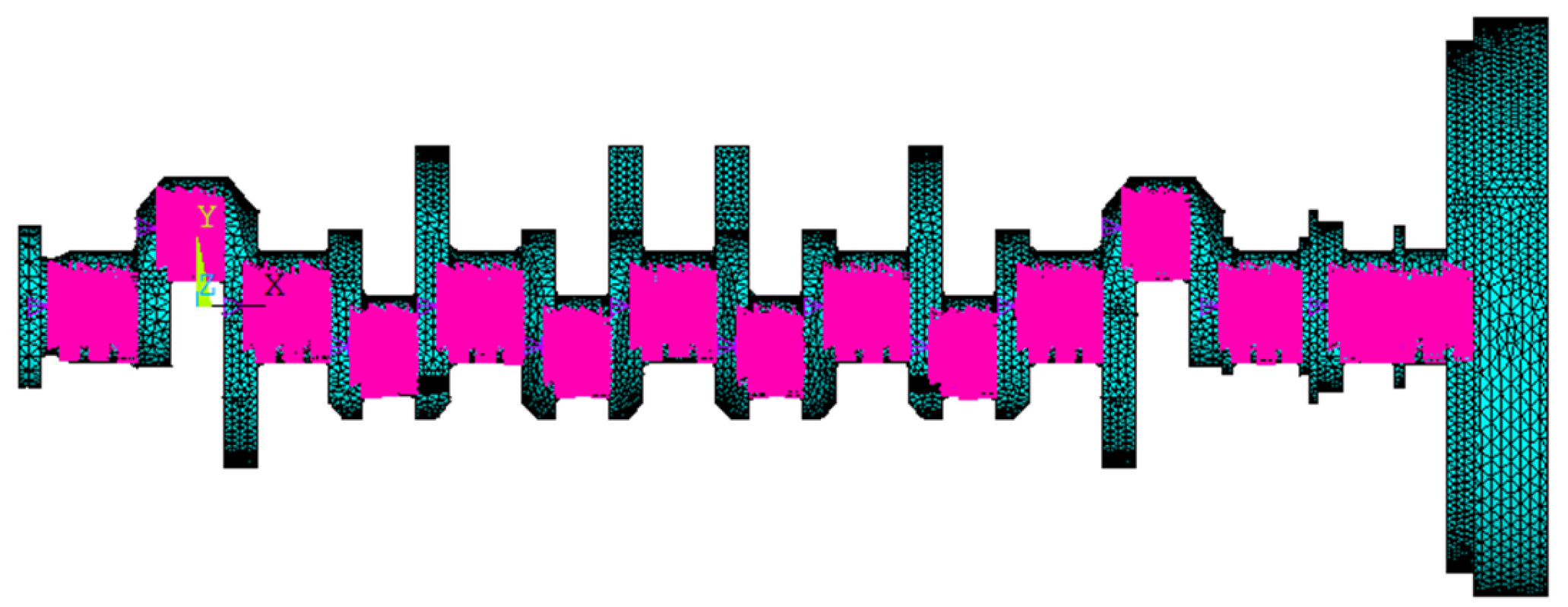
A finite element model of the crankshaft system is created using the commercial software ANSYS 19.2. The process of automatically defining master nodes, searching for nodes in the local vicinity of the master nodes, and defining coupled degrees of freedom is implemented through programme development to establish the substructure model of the diesel engine crankshaft system. Figure 3 illustrates the substructure model of the crankshaft system for a six-cylinder diesel engine. Figure 4 shows the results of establishing the coupling relationship between the degrees of freedom of the main and subsidiary nodes of the substructure model.

3. Calculation of Free Vibration of Crankshaft System Substructures

Due to the inherent characteristics of the structure’s free vibration response, the free vibration calculation method is presented here to verify whether the substructure model can accurately reflect the dynamic behaviour of the crankshaft system. A six-cylinder diesel engine crankshaft system is used as an example to assess whether the established substructure model can effectively replace the finite element model in dynamic calculations. The free vibration of its substructure dynamic model is formulated as a generalized eigenvalue–eigenvector problem, expressed as below:

$$(K-{\omega }^{2}M)\phi =0$$

(18)

To efficiently solve this problem, the symmetry of the mass and stiffness matrices is utilized, transforming the problem into a standard eigenvalue–eigenvector problem. First, the mass matrix is decomposed using Cholesky decomposition, which transforms the matrix into the following:

$$M=L_M{L}_M^T$$

(19)

where $L_M$ is a lower triangular matrix. The Equation (18) can then be further transformed into a standard semi-definite symmetric matrix eigenvalue problem, which is expressed as follows:

$$A\phi ={\omega }^2\phi$$

(20)

where $A=L_M^{-1}K{\left[L_M^{-1}\right]}^T$.

Since matrix $A$ is a semi-definite symmetric matrix, the Jacobi iteration method can be used for efficient solving. The updated formula for the Jacobi iteration method is

$${\phi }_{k+1}={\phi }_k-{\alpha }_k(A{\phi }_k-{\lambda }_k{\phi }_k)$$

(21)

where ${\lambda }_k$ is the eigenvalue at the $k$-th iteration, and ${\alpha }_k$ is the step factor. The system’s natural frequencies and corresponding mode shapes are ultimately obtained through multiple iterations.

Since the finite element model can accurately represent the mechanical properties of the crankshaft system, the results from the finite element method are used as the verification standard to assess the accuracy of the substructure model and associated numerical calculation methods. The calculations were performed considering different coupling region sizes, as shown in

Table 1. Parameter settings for different coupling regions.

Coupling Region Size	Radial Threshold	Axial Threshold
Moderate coupling region	d/3	d/20
Small coupling region	d/5	d/50

. The calculation results for the natural frequencies of the crankshaft’s free vibration are shown in

Table 2. Comparison of crankshaft-free vibration intrinsic frequency results under different modelling conditions. The main journals were defined using one and three master nodes, respectively, and the three master nodes were also selected to calculate smaller coupling regions.

Frequency Order	Take 1 Master Node and a Moderate Coupling Region (Hz)	Take 3 Master Nodes and a Moderate Coupling Region (Hz)	Take 3 Master Nodes and a Small Coupling Region (Hz)	ANSYS 19.2 Calculations (Hz)
1	28.946	29.874	29.209	30.85
2	30.186	31.238	30.461	32.38
3	77.591	80.103	79.259	80.307
4	83.034	86.236	84.135	86.754
5	91.382	93.684	91.407	95.053
6	140.508	145.361	141.203	143.42
7	151.237	156.025	154.349	152.89
8	168.614	175.562	171.268	160.93
9	224.381	233.316	226.185	229.62
10	258.979	268.536	261.762	266.52

. In the table, the main shaft necks are defined with one and three main nodes. Compared with previous studies, the validation results presented in this work are more convincing. The free vibration response was computed using Cholesky decomposition, and a detailed comparison was conducted with ANSYS 19.2 results by varying the number of master nodes and the size of the coupling region. These comparisons demonstrate the robustness and reliability of the proposed substructure modelling approach [27]. Compared to the model with one main node, the model with three main nodes demonstrates higher accuracy, with its natural frequencies being closer to those calculated using the ANSYS 19.2 finite element method.

4. Methods for Calculating the Dynamic Response of Crankshaft System Substructures

4.1. Crankshaft Substructure Forced Vibration Calculation Method

The Newmark method is commonly used for dynamic response calculations. However, the substructure model of the crankshaft system often still contains a large number of degrees of freedom. Due to factors such as the selection of master node positions and the distribution of mass and stiffness, significant parameter differences and frequency discrepancies may arise in the dynamic model, leading to coupled responses. This results in poor numerical performance due to stiffness and challenging accurate dynamic response calculations. To address this, the implicit Newmark method is employed for numerical integration, with a prediction-correction mechanism introduced for each time step. By iteratively optimizing the approximate solutions for displacement and velocity, local truncation errors are minimized, resulting in a more adaptable and reliable method for dynamic response calculation. The specific calculation method is as follows.

The Newmark-β method computes for each time step within the time interval $[t,t+\Delta t]$ as follows:

$$\widehat{K}=K+a_{0}M+a_{1}C$$

(22)

The effective load at the time $[t,t+\Delta t]$ is

$${\widehat{F}}_{t+\Delta t}=F_{t+\Delta t}+M(a_0{x}_t+a_2{\dot{x}}_t+a_3{\ddot{x}}_t)+C(a_1{x}_t+a_4{\dot{x}}_t+a_5{\ddot{x}}_t)$$

(23)

The effective displacement at the time $[t,t+\Delta t]$ is

$$\widehat{K}{x}_{t+\Delta t}=F_{t+\Delta t}$$

(24)

The velocity and acceleration at the time $[t,t+\Delta t]$ are

$${\dot{x}}_{t+\Delta t}={\dot{x}}_t+a_6{\ddot{x}}_t+a_7{\ddot{x}}_{t+\Delta t}$$

(25)

$${\ddot{x}}_{t+\Delta t}=a_0(x_{t+\Delta t}+x_t)-a_2{\dot{x}}_t-a_3{\ddot{x}}_t$$

(26)

where $\delta$ and $\beta$ are adjustable parameters based on accuracy and stability requirements. When $\delta \ge 1/2$, $\beta \ge 1/4(1/2+\delta {)}^2$, the Newmark-β method is unconditionally stable. Additionally, let

$$\begin{array}{l}{a}_0=1/(\beta \Delta t^2),a_1=\delta /(\beta \Delta t),a_2=1/(\beta \Delta t),a_3=1/2\beta -1,a_4=\delta /\beta -1,\\ a_5=\Delta t/2(\delta /\beta -2),a_6=\Delta t(1-\delta ),a_7=\delta \Delta t\end{array}$$

(27)

To address the local truncation error caused by high-frequency vibrations, each time step first computes the predicted displacement and then the corrected displacement. The predicted displacement is given by

$$q_{n+1}^{pred}=q_n+\Delta t{\dot{q}}_n+\Delta t^2({\displaystyle \frac{1}{2}}-\beta ){\ddot{q}}_n$$

(28)

The corrected displacement is obtained using iterative correction as follows:

$$q_{n+1}^{corr}=q_{n+1}^{pred}+\beta \Delta t^2{\ddot{q}}_{n+1}$$

(29)

The error assessment quantity E is defined as the difference between the two:

$$E=∥q_{n+1}^{corr}-q_{n+1}^{pred}∥$$

(30)

The error reflects the truncation error or the lack of iterative correction due to high-frequency modes in the current time step. The time step is adjusted according to the comparison of the error $E$ with the preset tolerance error $\mathcal{E}$. The following update formula is used:

$$\Delta t_{new}=\Delta t({\displaystyle \frac{\epsilon }{E}}{)}^{\frac{1}{p}}$$

(31)

where $p$ is the order of integration; for the Newmark method take $p$ = 2; $\mathcal{E}$ is the set error tolerance—take $\mathcal{E}$ = 0.05.

When $E\ge \epsilon$, it indicates that the local truncation error is large and $\Delta t$ should be reduced,

When $E\ll \epsilon$, $\Delta t$ can be increased appropriately to improve the computational efficiency.

In the nonlinear iterative solution at each time step, a dynamic relaxation factor ${\omega }_k$ is added to correct the updating formulae to prevent instability caused by too large corrections:

$$q_{n+1}^{(i+1)}=q_{n+1}^{\left(i\right)}+{\omega }_k\Delta q_{n+1}^{\left(i\right)}$$

(32)

where $\Delta q_{n+1}^{\left(i\right)}$ is the displacement correction obtained in the $i$-th iteration. This treatment effectively suppresses excessive corrections caused by high-frequency modes, ensuring iterative convergence.

The dynamic relaxation factor ${\omega }_k$ is defined as

$${\omega }_k={\displaystyle \frac{1}{1+\alpha \Delta t}}$$

(33)

where the parameter $\alpha$ is related to the system’s stiffness and damping characteristics.

When the time step is small, ${\omega }_k$ tends to have a smaller value, thereby reducing the correction magnitude.

When the time step is large, ${\omega }_k$ approaches 1, allowing for more thorough iterative corrections.

At each time step, to solve for ${\ddot{q}}_{n+1}$ and update $q_{n+1}$, it is usually necessary to construct the “effective stiffness matrix”. For classical problems, it can be represented as

$$K_{eff}={\displaystyle \frac{1}{\beta \Delta t^2}}M+{\displaystyle \frac{\gamma }{\beta \Delta t}}C+K$$

(34)

To perform order reduction, corrections need to be made, and the iterative update formula is

$$q_{n+1}^{(i+1)}=q_{n+1}^{\left(i\right)}+{\omega }_k{K}_{eff}{R}_{n+1}^{\left(i\right)}$$

(35)

where the residual $R_{n+1}^{\left(i\right)}$ is defined as

$$R_{n+1}^{\left(i\right)}=f_{n+1}-(M{\ddot{q}}_{n+1}^{\left(i\right)}+C{\dot{q}}_{n+1}^{\left(i\right)}+KC{q}_{n+1}^{\left(i\right)})$$

(36)

By adjusting the dynamic relaxation factor, the correction amount for each iteration can be controlled, ensuring the convergence of the iteration process and improving computational efficiency.

Building on the improved Newmark method, a dynamic calculation tool was designed and developed to perform numerical computations for the crankshaft system’s substructure dynamic model. This tool can compute the diesel engine crankshaft system’s torsional, longitudinal, and lateral vibration characteristics under various operating conditions. It can also assess vibration responses under conditions such as changes in rotational speed and load fluctuations, making it valuable for evaluating and studying the crankshaft system’s vibration behaviour.

4.2. Verification of Dynamic Response Calculation Results

This paper introduces a dynamic relaxation factor, integrating it with an energy gradient-based Newmark adaptive integration algorithm to calculate dynamic responses. To verify the accuracy of the established substructure dynamic model, a six-cylinder diesel engine at 1200 RPM is used as a test case. Under the same boundary and loading conditions, the dynamic programme based on the substructure method is compared with the coupled vibration response from the ABAQUS finite element model. The programme’s computation time is reduced by 75% compared to ABAQUS. The calculation results are shown in Figure 5, Figure 6 and Figure 7, with the following findings:

(1)

The results from both methods align well regarding the main frequencies and amplitudes, indicating that the programme is relatively reliable.

(2)

The substructure dynamic calculation programme provides richer frequency components with a more detailed description of high-frequency harmonics.

(3)

The programme’s results show noticeable interference in the torsional response for certain time periods, smoothing one peak. This phenomenon arises because the substructure model includes components beyond the observed direction, resulting from torsional, bending, and longitudinal vibration coupling.

(4)

Due to the proximity of the bearing installation positions to the flywheel end, the bending vibration amplitudes in all directions at the flywheel end are relatively small compared to the torsional vibration amplitude. This is because the nearby bearing support provides greater structural constraint, effectively limiting bending deformation in that region. As a result, the dynamic response at the flywheel end is dominated by torsional behaviour, while bending contributions remain minimal under the same loading conditions.

5. Study of Factors Influencing Dynamic Response of Crankshaft System

Establishing the crankshaft subsystem model and its dynamic calculations involve many parameters that may affect the computational results. This study explores the influence of different parameters, including integration step size, number of master nodes, coupling region size, and crankshaft support stiffness, on the results. The analysis primarily focuses on the difference in torsional angles at both ends, which reflects the torsional response, and the lateral rotational angle of the flywheel, which represents the bending vibration response.

5.1. Integration Step Size

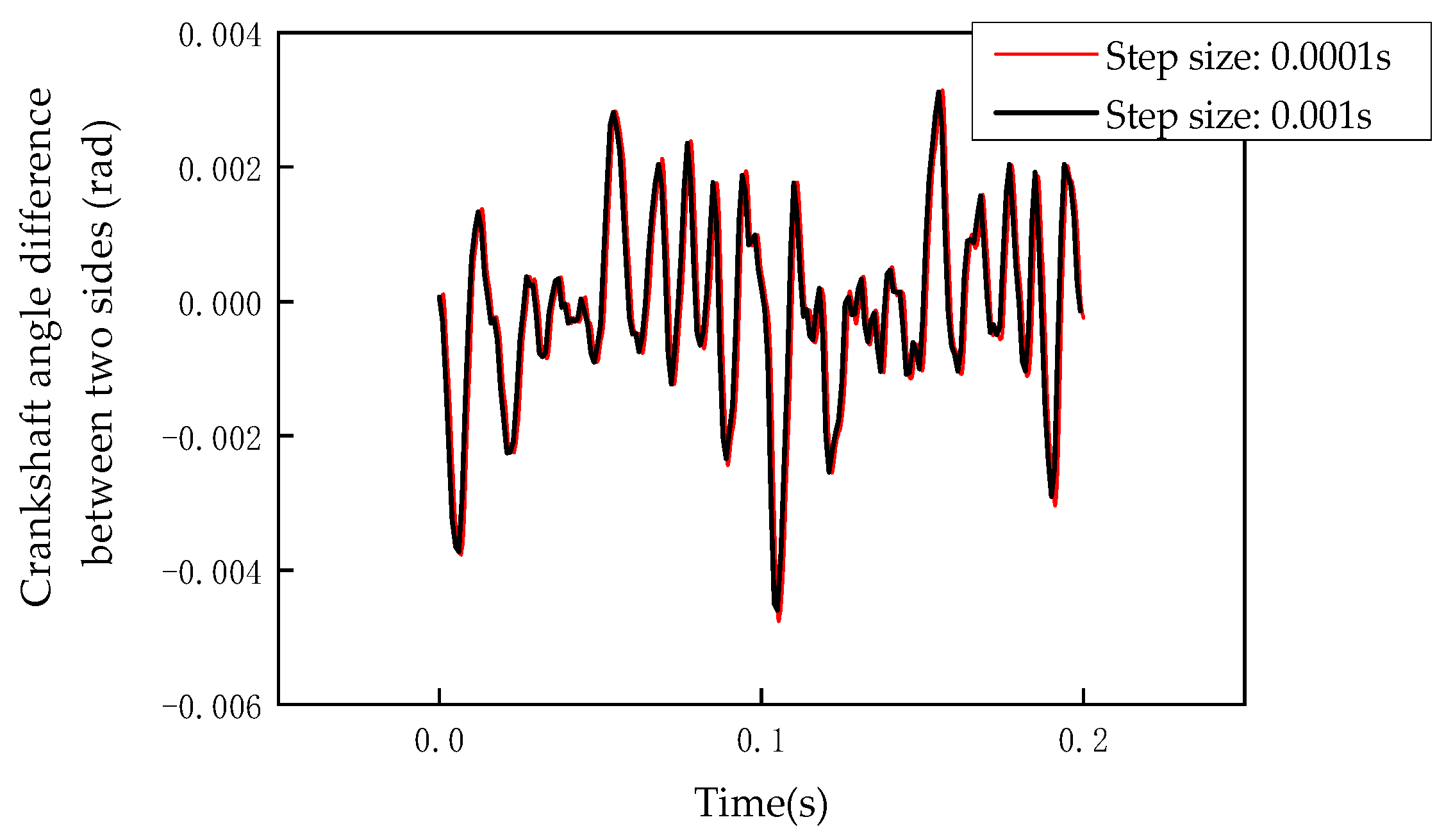
Figure 8 and Figure 9 present the response results under various initial step sizes. The comparison reveals that, despite variations in step size, the overall response trends remain consistent. This indicates that changes in the initial step size have a minimal impact on the primary response characteristics. However, a huge time step may suppress high-frequency components. Therefore, selecting an appropriate time step is essential to balance computational accuracy and efficiency. For dynamic problems characterized by significant high-frequency content, employing a smaller initial step size in conjunction with an adaptive strategy can enhance accuracy and stability.

5.2. Selection of the Number of Main Nodes

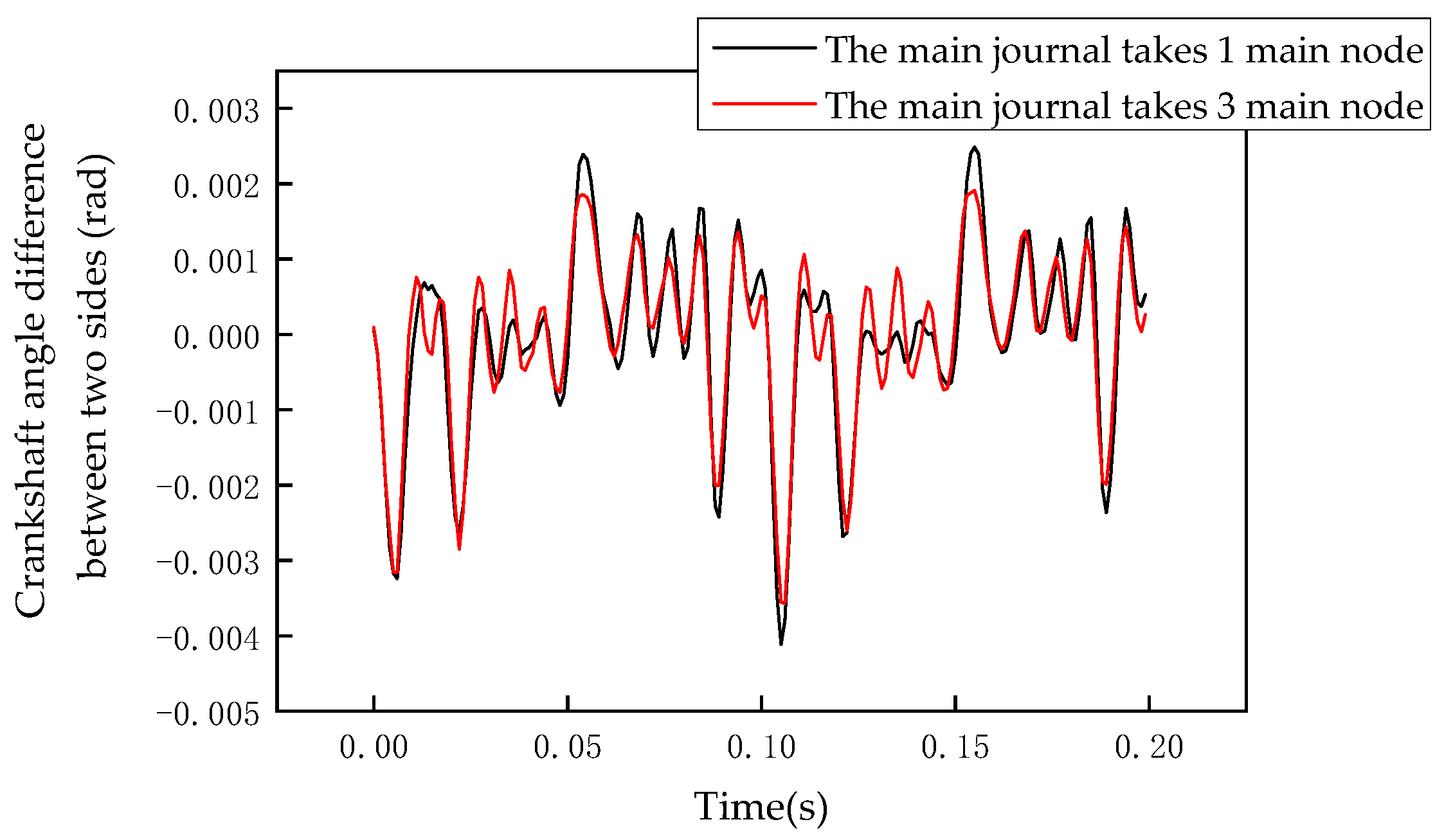
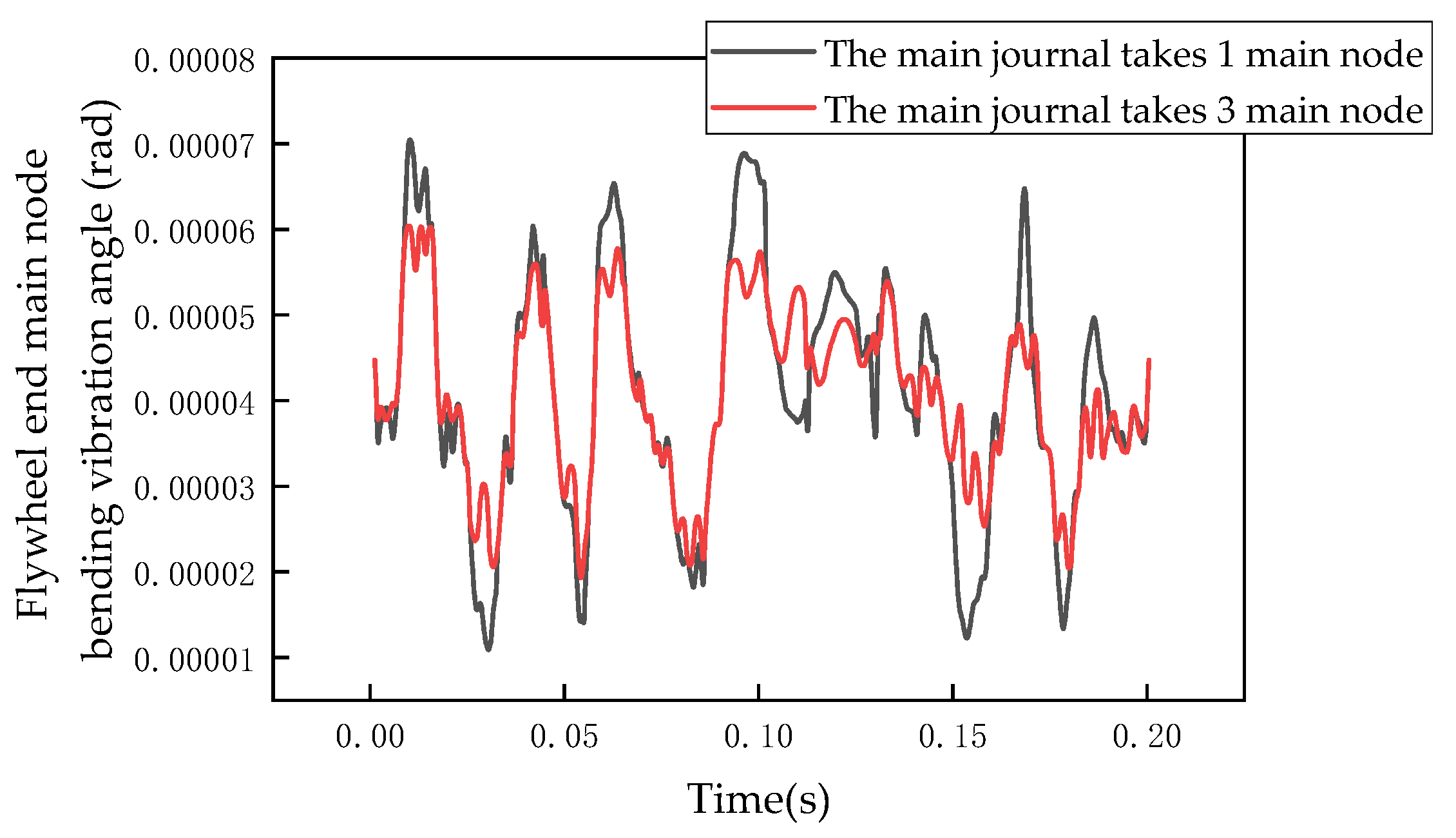
Figure 10 and Figure 11 present the response results of the spindle journal using different numbers of master nodes. Both cases’ frequencies and primary amplitudes are generally consistent, indicating that increasing the number of master nodes does not significantly affect the overall response. A single master node is sufficient to capture the main dynamic characteristics of the system. Although the three-node configuration improves the resolution of certain local features, the overall error remains minimal.

Regarding local response, the curve from the three-node configuration offers a more refined representation, exhibiting slight variations in fluctuation patterns within high-frequency vibration regions, particularly near peaks and troughs. These refinements contribute to a reduction in numerical error. As previously noted, the substructure with one master node has a slightly lower natural frequency, resulting in a marginally higher response amplitude than the three-node case. Increasing the number of master nodes may also enhance the suppression of high-frequency components at specific time points.

5.3. Degree of Freedom Coupling Region

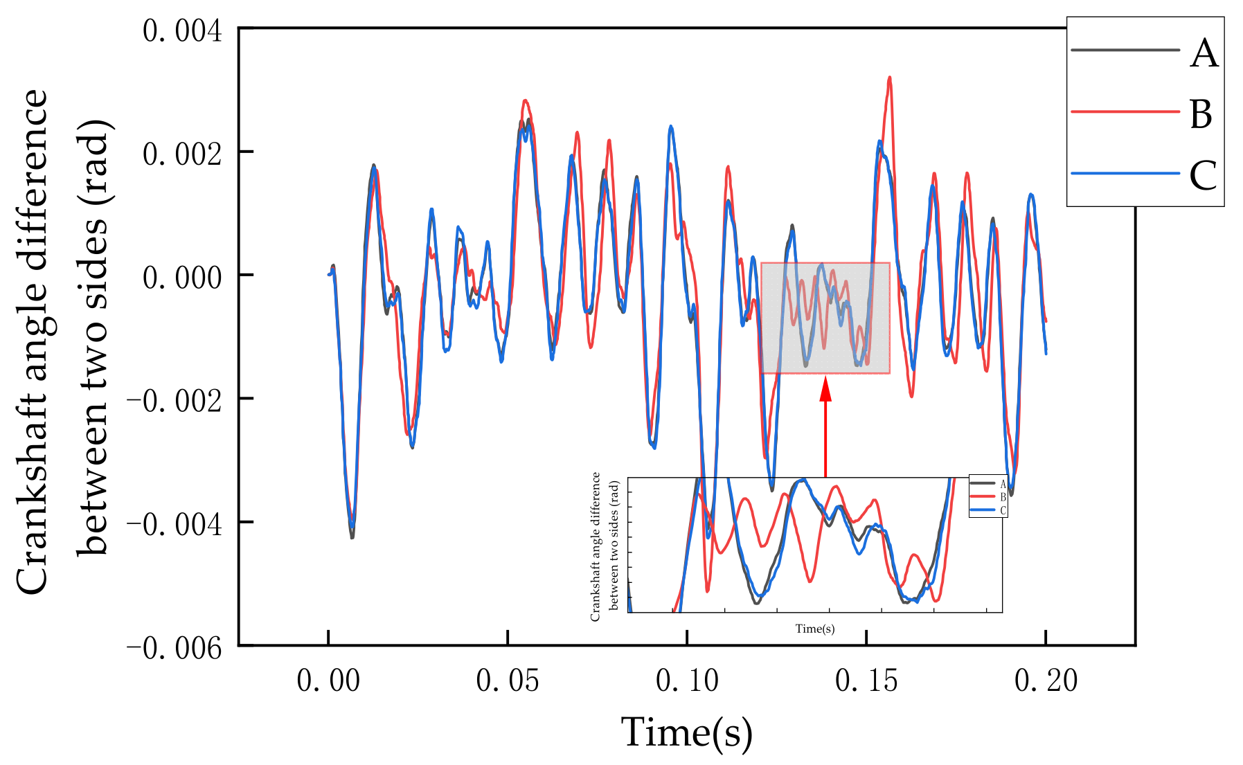
Figure 12 and Figure 13 illustrate the response results for varying coupling region sizes, defined in terms of degrees of freedom. The corresponding threshold values are listed in

Table 3. Threshold setting for different coupling regions.

Curved Line	Radial Threshold	Axial Threshold
A	d/3	d/20
B	d/5	d/50
C	2d/3	d/10

where d denotes the spindle diameter. Curve B, which corresponds to a smaller coupling region and lower crankshaft stiffness, exhibits more detailed high-frequency content but also higher oscillation amplitudes. In contrast, Curves A and C show more consistent behaviour. In particular, Curve C, with its larger coupling region and increased stiffness, results in slightly reduced amplitude.

In practical computations, smaller coupling regions tend to be more sensitive to high-frequency excitation. Moderately enlarging the coupling region can enhance the accuracy of the substructure’s dynamic model. However, if the area becomes too large, excessive smoothing of high-frequency vibrations may occur, diminishing the resolution of local response features.

5.4. Bearing Support Stiffness

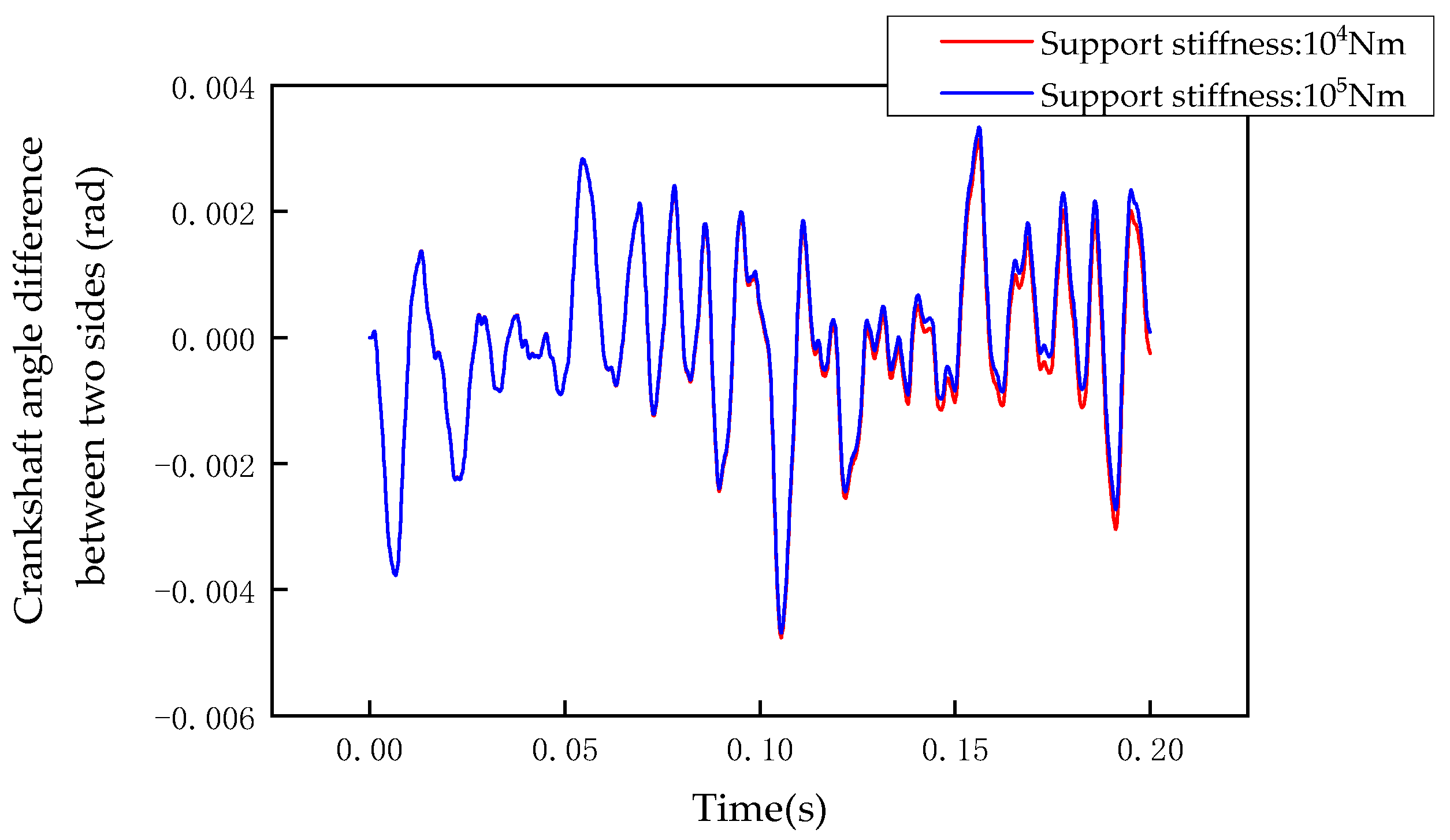
The bearing support stiffness in marine diesel engine crankshaft systems typically ranges from 10⁴ to 10⁵ Nm. Figure 14 presents the response results for different support stiffness values. A stiffness of 10⁵ Nm, compared to 10⁴ Nm, represents a stronger boundary constraint. The increased stiffness restricts motion at the boundary points, leading to a local upward shift in the response and reducing the accuracy of the results. In practical computations, it is essential to consider factors such as bearing housing deformation, bearing clearance, and lubrication conditions. A support stiffness value between one-third and one-fifth of the relative torsional stiffness on both sides of the crankshaft is recommended to ensure computational stability and to minimize the impact on the system’s modal characteristics.

6. Conclusions

This study systematically presents the dynamic modelling and corresponding numerical solution methods based on the substructure model for the complex vibration problem of torsional, bending, and longitudinal coupling in the diesel engine crankshaft system. It also explores the impact of various modelling factors on the vibration of the diesel engine crankshaft system. The research provides valuable support and references for the diesel engine crankshaft system’s design, analysis, and application. The main conclusions drawn from the study are as follows:

(1)

The crankshaft substructure model was effectively established by setting predefined thresholds to construct coupling constraints between the main and auxiliary nodes and performing degree-of-freedom reduction. This method significantly reduces the computational degrees of freedom while retaining the primary dynamic characteristics of the system.

(2)

The Cholesky decomposition and Jacobi iterative methods were found to accurately and efficiently solve the free vibration of the crankshaft system, demonstrating that the substructure model can effectively replace the finite element model. Additionally, increasing the number of main nodes helps improve model accuracy.

(3)

Under the framework of the implicit Newmark-β method, the combination of a prediction-correction mechanism and dynamic relaxation factors to adjust the iterative convergence path, along with an adaptive time step strategy driven by energy gradients, can effectively balance numerical stability and the capture of high-frequency response details.

(4)

In dynamic response calculations, appropriately increasing the number of main nodes, reducing the time step size, and narrowing the coupling region enhance the description of high-frequency local vibration details. Increasing the coupling region can more accurately reflect the dynamic properties of the structure.

(5)

Using a smaller initial step size combined with the energy gradient criterion for adaptive step size can optimize computational accuracy and efficiency. An increase in support stiffness will cause an upward shift in the local response results.

With the development of the substructure dynamic response calculation programme, it becomes feasible to conduct many simulations through various case studies. This enables a deeper investigation into the characteristics of coupled vibrations and the interaction mechanisms among torsional, bending, and axial vibration modes. By identifying underlying patterns and dynamic behaviour, the method provides valuable technical support for fundamental diesel engine design and shaft system development.

References

1. Gomes, J.; Gaivota, N.; Martins, R.F.; Silva, P.P. Failure analysis of crankshafts used in maritime V12 diesel engines. Eng. Fail. Anal. 2018, 92, 466–479. [Google Scholar] [CrossRef]
2. Deng, X.; Zhang, B. Summary on Torsional Vibration of Crankshaft System in Internal Combustion Engines. Automob. Parts 2012, 1, 76–78. [Google Scholar]
3. Kimura, J.; Kobayashi, S.; Hoshina, K.; Kawase, K.; Matsui, K.; Yamamoto, A. Crankshaft Impact Noise and Three-Dimensional Vibration; 0148-7191; SAE Technical Paper; SAE International: Warrendale, PA, USA, 2014. [Google Scholar]
4. Tsitsilonis, K.M. A Systematic Methodology Enabling Marine Engine Health Assessment by Employing First-Principles Digital Twins. Ph.D. Thesis, University of Strathclyde, Glasgow, UK, 2023. [Google Scholar]
5. Carrera, E.; Pagani, A.; Petrolo, M.; Zappino, E. Recent developments on refined theories for beams with applications. Mech. Eng. Rev. 2015, 2, 14–00298-00214-00298. [Google Scholar] [CrossRef]
6. Hurty, W.C. Dynamic analysis of structural systems using component modes. AIAA J. 1965, 3, 678–685. [Google Scholar] [CrossRef]
7. Craig Jr, R.R.; Bampton, M.C. Coupling of substructures for dynamic analyses. AIAA J. 1968, 6, 1313–1319. [Google Scholar] [CrossRef]
8. Wang, F.; Luo, G.-H.; Yan, S.; Cui, H.-T. A Comparison Study on Co-and Counterrotating Dual-Rotor System with Squeeze Film Dampers and Intermediate Bearing. Shock. Vib. 2017, 2017, 5493763. [Google Scholar] [CrossRef]
9. Wang, F.; Luo, G.-H.; Yang, X.-G.; Cui, H.-T. Research on modeling and dynamic characteristics of complex coaxial rotor system. J. Vibroengineering 2017, 19, 1524–1545. [Google Scholar] [CrossRef]
10. Zhai, Y.-J.; Ma, Z.-S.; Chang, H.-Z.; Ding, Q. Model order reduction and dynamic characteristic analysis of the bolted flange structure with free-free boundaries. Structures 2021, 34, 149–157. [Google Scholar] [CrossRef]
11. Gao, F.; Sun, W. Reduced-order modeling for and vibration characteristics analysis of a hard-coated mistuned blisk. Coatings 2017, 7, 103. [Google Scholar] [CrossRef]
12. Zheng, Z.; Xie, Y.; Zhang, D. Reduced-order modeling for stability and steady-state response analysis of asymmetric rotor using three-dimensional finite element model. J. Eng. Gas Turbines Power 2019, 141, 101001. [Google Scholar] [CrossRef]
13. Hou, S. Review of modal synthesis techniques and a new approach. Shock. Vib. Bull. 1969, 40, 25–39. [Google Scholar]
14. Wang, T.; Cheng, C.; Guo, X. Model-based predicting and correcting algorithms for substructure online hybrid tests. Earthq. Eng. Struct. Dyn. 2012, 41, 2331–2349. [Google Scholar] [CrossRef]
15. Huang, D.; Liu, Y.; Liu, H.; Yi, J. Resonances of elastic rotor induced by roller bearing with consideration of cage vibration. Proc. Inst. Mech. Eng. Part K J. Multi-Body Dyn. 2018, 232, 446–456. [Google Scholar] [CrossRef]
16. Yu, Y.; Jin, X.; Fu, Y.; Zhao, T. Study on the coupled vibration characteristics of a two-stage bladed disk rotor system. Appl. Sci. 2021, 11, 8600. [Google Scholar] [CrossRef]
17. Ying, L.; Hongguang, L.; Yue, L. Accelerated parametric model order reduction method. J. Aerosp. Power 2019, 34, 2264–2270. [Google Scholar]
18. Ying, L.; Hongguang, L.; Yun, L. A component-based parametric model order reduction method. J. Vib. Shock 2020, 39, 148–154. [Google Scholar]
19. Bai, B.; Bai, G.-c. Dynamic probabilistic analysis of stress and deformation for bladed disk assemblies of aeroengine. J. Cent. South Univ. 2014, 21, 3722–3735. [Google Scholar] [CrossRef]
20. Bai, B.; Bai, G.C.; Li, C. Application of multi-stage multi-objective multi-disciplinary agent model based on dynamic substructural method in Mistuned Blisk. Aerosp. Sci. Technol. 2015, 46, 104–115. [Google Scholar] [CrossRef]
21. Bai, B.; Li, H.; Zhang, W.; Cui, Y. Application of extremum response surface method-based improved substructure component modal synthesis in mistuned turbine bladed disk. J. Sound Vib. 2020, 472, 115210. [Google Scholar] [CrossRef]
22. Géradin, M.; Rixen, D.J. A ‘nodeless’ dual superelement formulation for structural and multibody dynamics application to reduction of contact problems. Int. J. Numer. Methods Eng. 2016, 106, 773–798. [Google Scholar] [CrossRef]
23. Wu, Z.; Xia, L.; Wang, S.; Shi, T. Topology optimization of hierarchical lattice structures with substructuring. Comput. Methods Appl. Mech. Eng. 2019, 345, 602–617. [Google Scholar] [CrossRef]
24. Weng, S.; Zhu, H.; Xia, Y.; Li, J.; Tian, W. A review on dynamic substructuring methods for model updating and damage detection of large-scale structures. Adv. Struct. Eng. 2020, 23, 584–600. [Google Scholar] [CrossRef]
25. Mourelatos, Z.P. A crankshaft system model for structural dynamic analysis of internal combustion engines. Comput. Struct. 2001, 79, 2009–2027. [Google Scholar] [CrossRef]
26. Besset, S.; Jezequel, L. Dynamic substructuring based on a double modal analysis. J. Vib. Acoust. 2008, 130, 011008. [Google Scholar] [CrossRef]
27. Tian, Z.; Li, J.; Lin, X.; Hu, P. Research on generating technology of diesel engine crankshaft substructure dynamic model. Manuf. Autom. 2022, 44, 21–24+60. [Google Scholar]
Figure 1. Schematic diagram of the main nodes of the crankshaft substructure.
Applsci 15 05551 g001
Figure 2. Degree of freedom coupling schematic.
Applsci 15 05551 g002
Figure 3. Crankshaft system substructure generated by command flow.
Applsci 15 05551 g003
Figure 4. Master node and subsidiary node coupling relationship establishment.
Applsci 15 05551 g004
Figure 5. (a) Calculation results of the programme for the difference in axial angle between the two ends of the crankshaft; (b) ABAQUS calculation results of axial angle difference between the two ends of the crankshaft.
Applsci 15 05551 g005
Figure 6. (a) Flywheel end main node around the transverse axis of symmetry angle procedure calculation results; (b) Flywheel end main node around the transverse axis of symmetry ABAQUS calculation results.
Applsci 15 05551 g006
Figure 7. (a) Flywheel end main node bending vibration angle programme calculation results; (b) flywheel end main node bending vibration angle ABAQUS calculation results.
Applsci 15 05551 g007
Figure 8. Calculation results of angle difference between the two sides of the crankshaft for different initial steps.
Applsci 15 05551 g008
Figure 9. Calculated bending vibration angle of the main node at flywheel end with different initial steps.
Applsci 15 05551 g009
Figure 10. Calculation results of angle difference between the two sides of the crankshaft for the main journal taking different numbers of main nodes.
Applsci 15 05551 g010
Figure 11. Calculation results of the bending vibration angle of the main node at the flywheel end of the spindle neck taking different numbers of main nodes.
Applsci 15 05551 g011
Figure 12. Calculation results of angle difference between the two sides of the crankshaft for different coupling region sizes.
Applsci 15 05551 g012
Figure 13. Calculated bending vibration angle of the main node at the flywheel end with different coupling region sizes.
Applsci 15 05551 g013
Figure 14. Calculation results of angle difference between two sides of the crankshaft with different bearing support stiffnesses.
Applsci 15 05551 g014