
Evaluation of Thermal Damage Effect of Forest Fire Based on Multispectral Camera Combined with Dual Annealing Algorithm

Abstract
1. Introduction
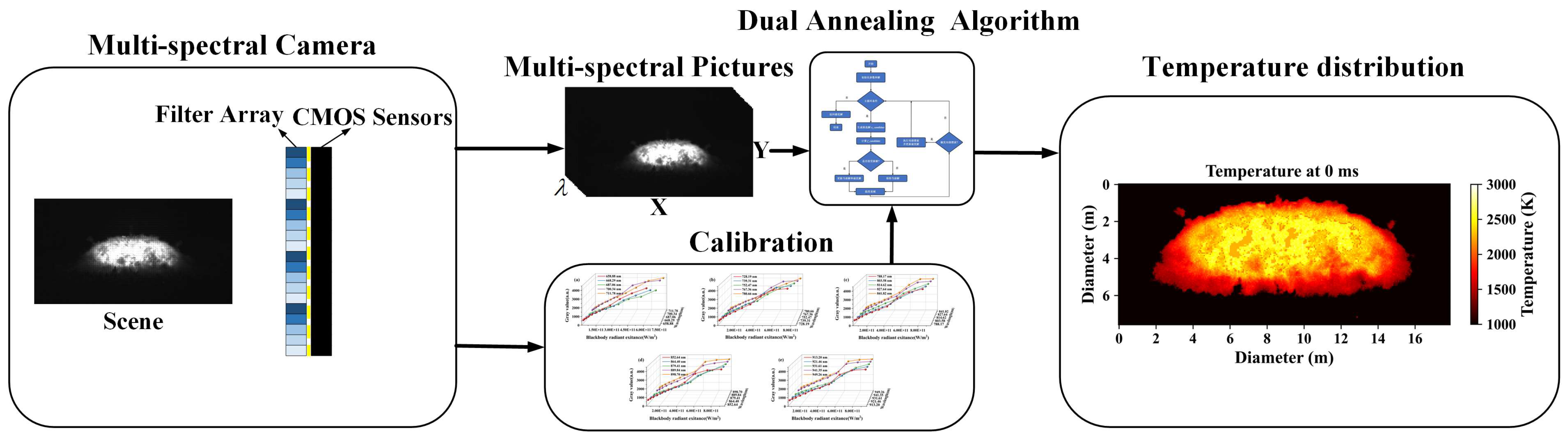
2. Methods
2.1. Multispectral Radiometric Thermometry
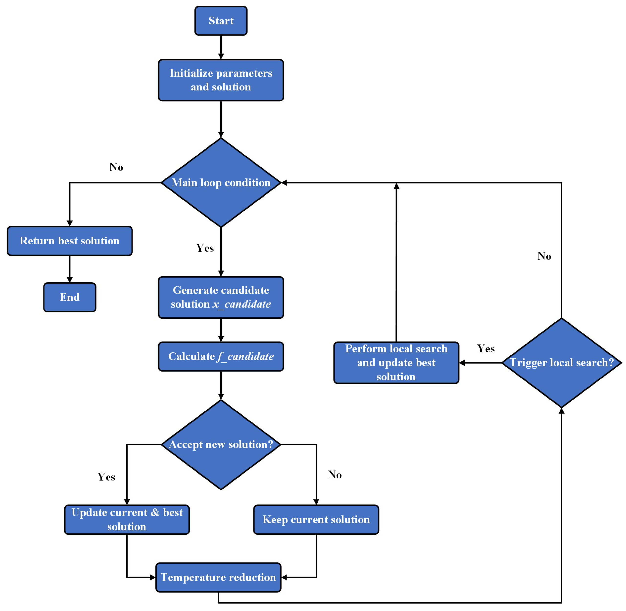
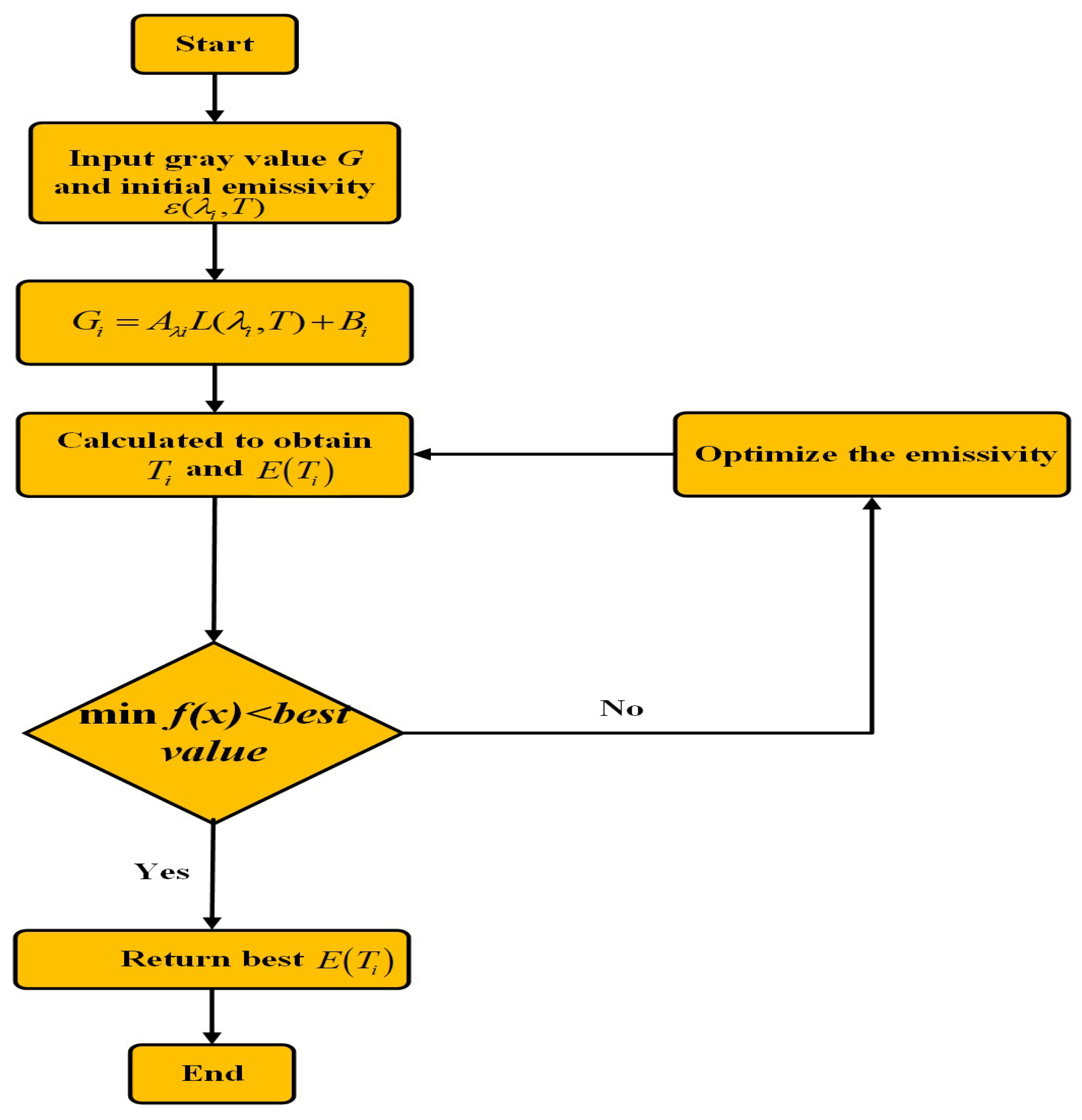
2.2. Dual Annealing Algorithm
| Algorithm 1: Dual Annealing algorithm |
| Input: - Objective function f(x) - Variable bounds [lower, upper] - Max iterations: maxiter - Initial temperature: T0 = 5230.0 - Restart temperature ratio: restart_temp_ratio = 2 × 10⁻⁵ - Visiting parameter: visit = 2.62 (controls perturbation distribution) - Acceptance parameter: accept = −5.0 (controls acceptance probability) - The maximum number of function calls: maxfun = 1 × 10⁷ Output: - Optimal solution x_best - Optimal value f_best Algorithmic flow A. Initialization: a. Parse bounds to generate lower and upper arrays. b. Compute restart temperature threshold: temperature_restart = T0 × restart_temp_ratio c. Generate initial solution: - If x0 is provided: x_current = x0 - Else: Randomly generate x_current ∈ [lower, upper] - Compute initial energy: f_current = f(x_current) d. Initialize best solution: x_best = x_current, f_best = f_current e. Initialize temperature decay parameters: - t1 = 2 visit−1− 1 - Current iteration step: s = 2.0 f. Initialize counters: - Not-improved counter: not_improved_idx = 0 - Function evaluations: nfev = 1 B. Main Loop (until iteration ≥ maxiter or T < temperature_restart): a. Compute current temperature: T = T0 × t1/(svisit−1 − 1) s = s + 1.0 b. Strategy Chain Loop (explore perturbations for each variable): for j = 0 to 2 × dim (dim = number of variables): i. Generate candidate solution x_candidate: - If j < dim: Global perturbation (all variables change) Δx = visit_fn(T) // Perturbation using distorted Cauchy-Lorentz distribution x_candidate = x_current + Δx x_candidate = lower + (x_candidate − lower) mod bound_range // Boundary handling - Else: Single-variable perturbation (only the (j−dim)-th variable changes) Apply perturbation to one variable as above ii. Evaluate candidate energy: f_candidate = f(x_candidate), nfev += 1 iii. Acceptance criterion: if f_candidate < f_current: Accept solution: x_current = x_candidate, f_current = f_candidate if f_current < f_best: Update best: x_best = x_current, f_best = f_current Reset counter: not_improved_idx = 0 else: delta_energy = f_candidate − f_current pqv_temp = 1 − (1 − accept) × delta_energy/T pqv = exp(ln(pqv_temp)/(1 − accept)) if pqv_temp > 0 else 0 if rand() < pqv: Accept solution: x_current = x_candidate, f_current = f_candidate iv. Termination check: If nfev ≥ maxfun, terminate. v. Update counter: not_improved_idx += 1 c. Trigger Local Search (enhance local optimization): - If not_improved_idx ≥ 1000 or exp(K× (f_best − f_current)/T) ≥ rand(): i. Call local optimizer (L-BFGS-B) from x_best to get x_local and f_local ii. If f_local < f_best: Update x_best = x_local, f_best = f_local iii. Reset counter: not_improved_idx = 0 d. Temperature Restart: - If T < temperature_restart: Reinitialize x_current and reset T = T0 C. Return results: - x_best, f_best |
- Perturbation GenerationBased on a modified Cauchy-Lorentz distribution, where the “visit” parameter controls the perturbation magnitude.
- Acceptance ProbabilityThe accept parameter adjusts tolerance for inferior solutions to avoid premature convergence in local optima.
- Local SearchEnhances local optimization capability after global exploration, improving convergence efficiency.
- Temperature RestartPeriodically resets temperature and solutions to prevent premature convergence.
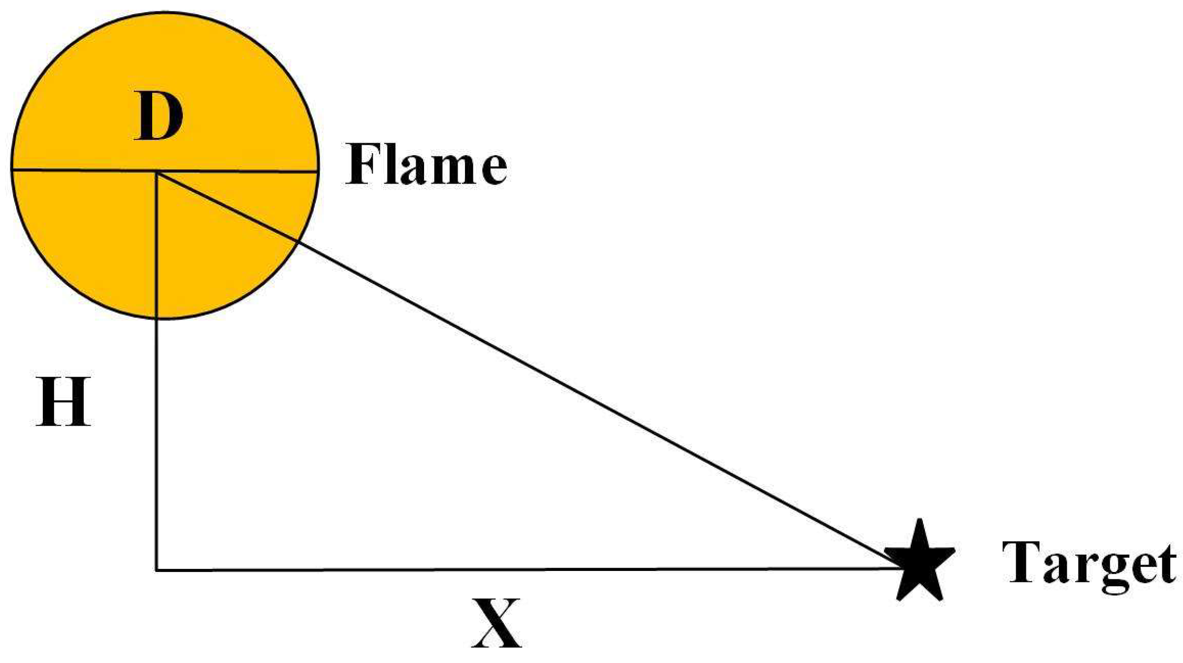
2.3. Dynamic Fire Thermal Damage Assessment Model
3. Results
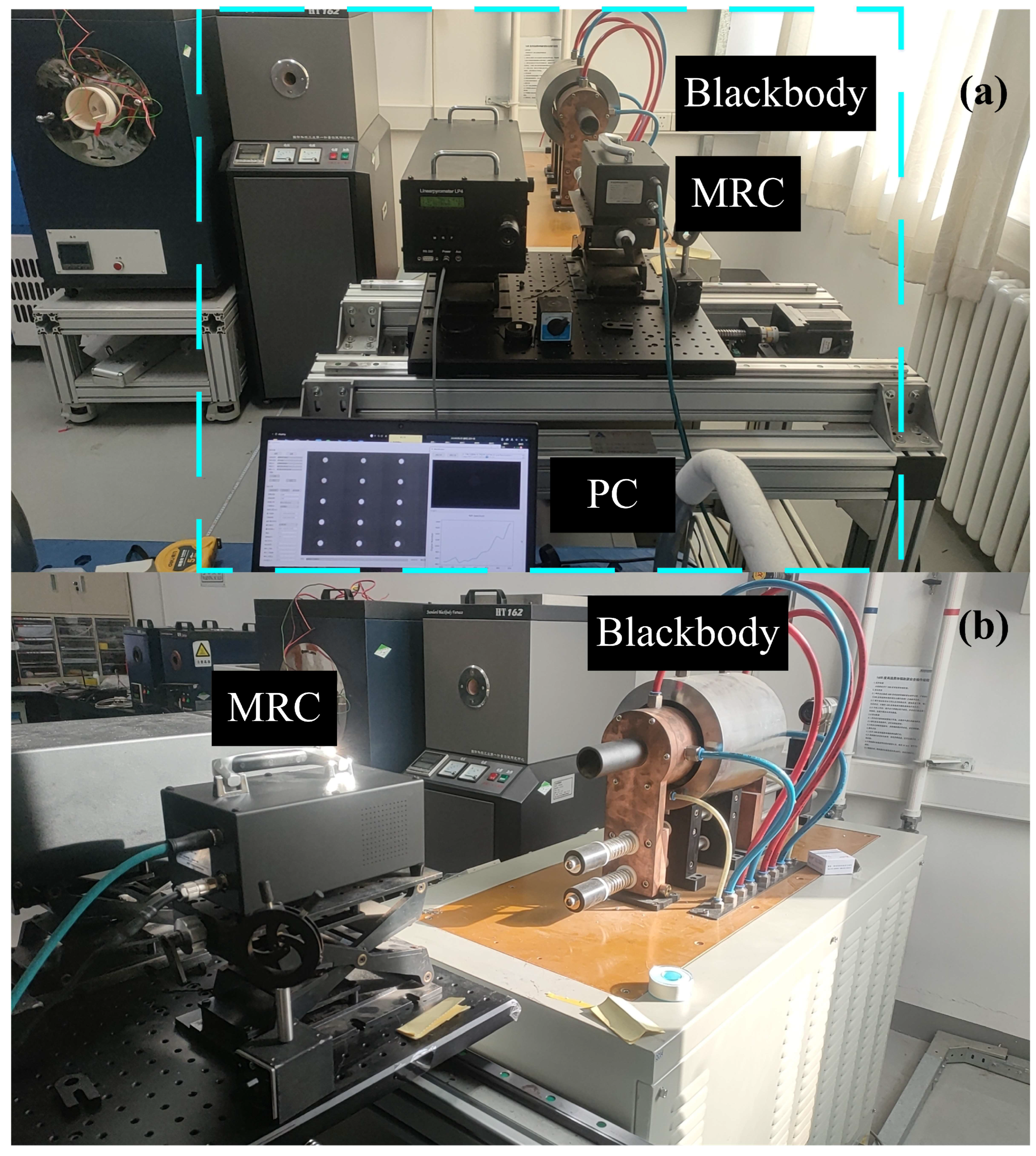
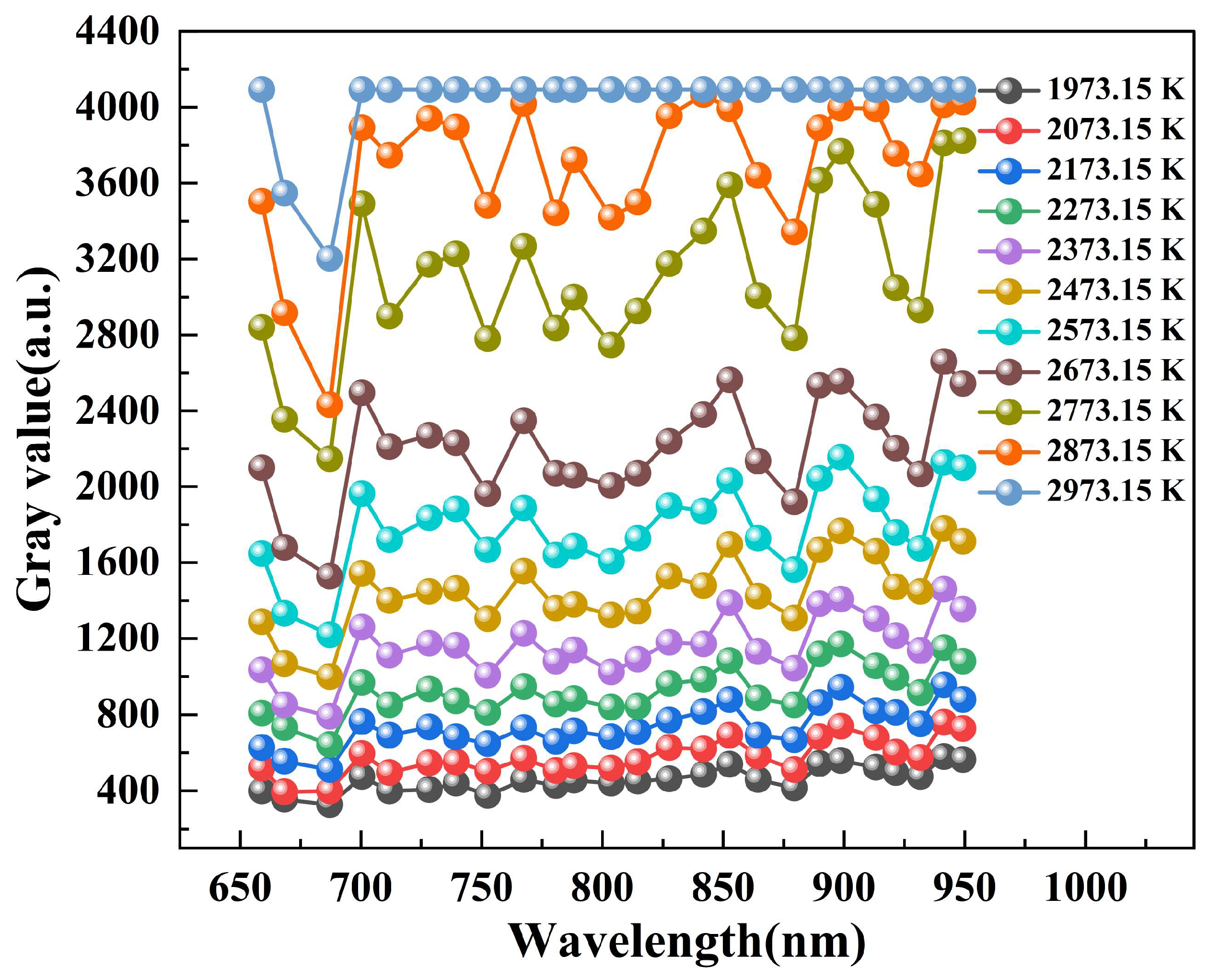
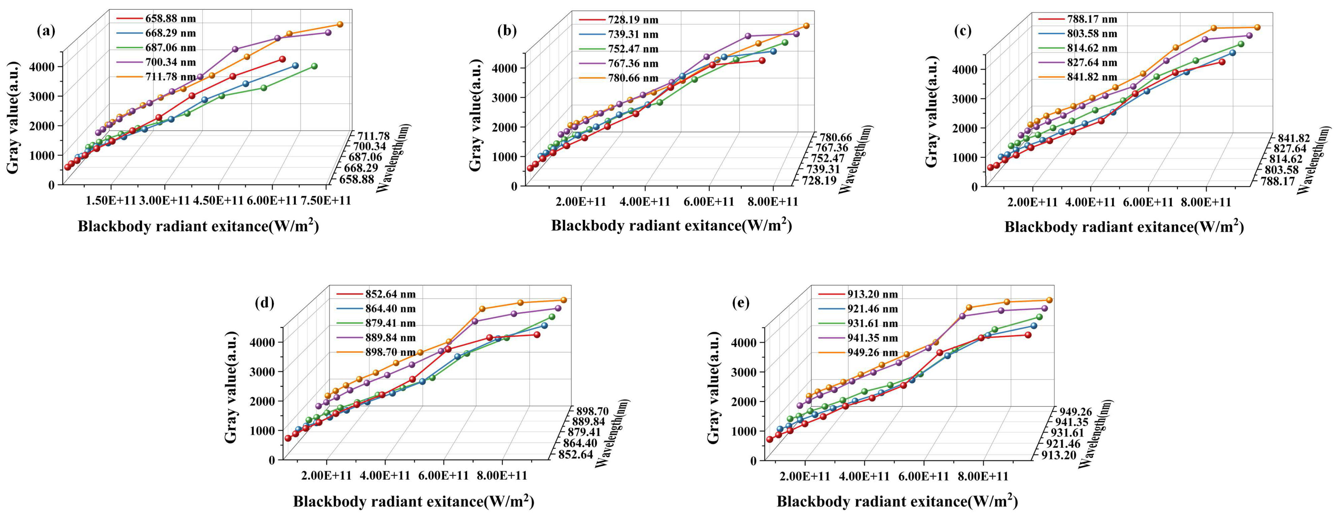
3.1. Blackbody Furnace Temperature Calibration Experiment
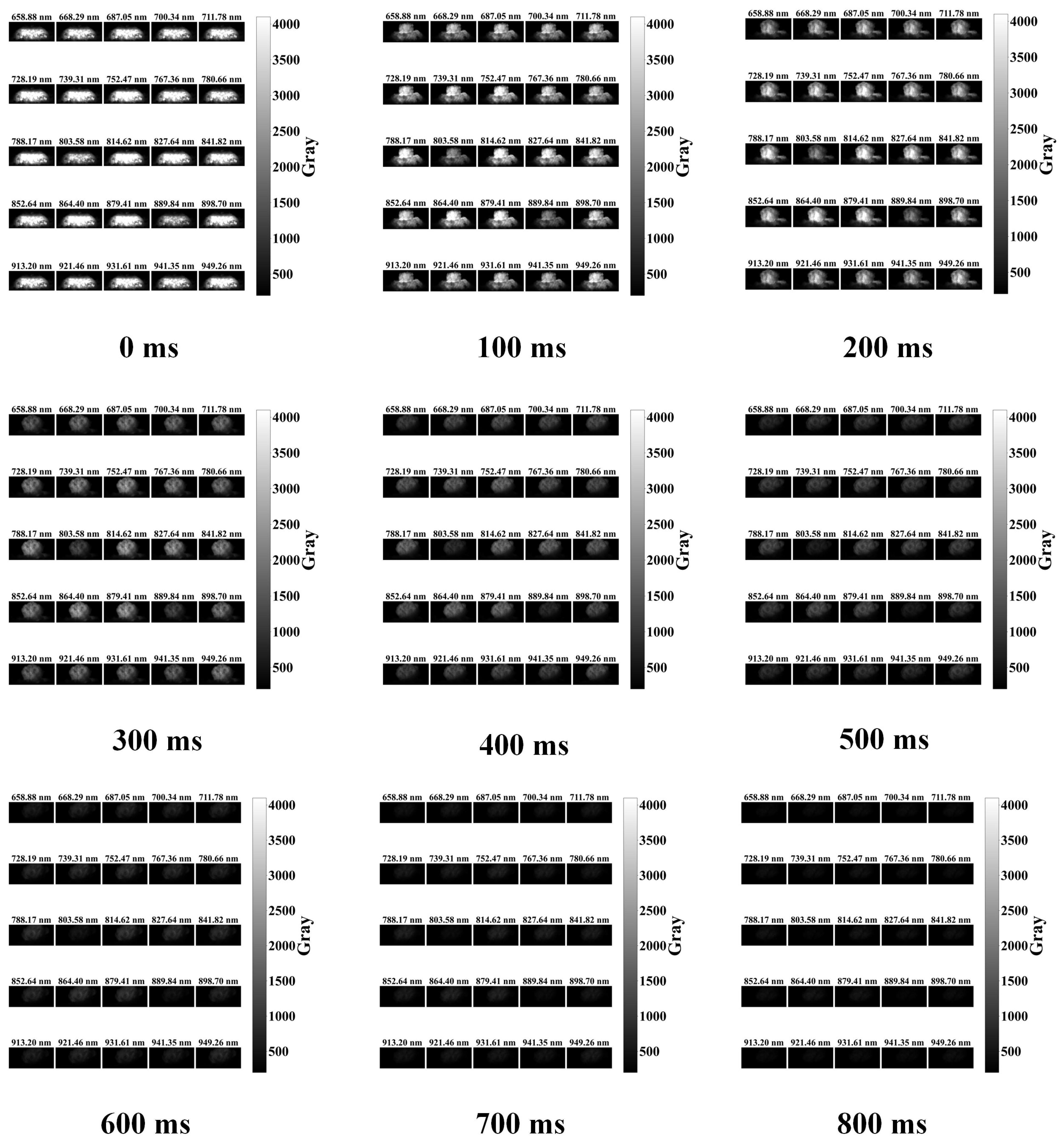
3.2. Simulated Flame Temperature Measurement and Thermal Damage Assessment
4. Discussion
5. Conclusions
Author Contributions
Funding
Institutional Review Board Statement
Informed Consent Statement
Data Availability Statement
Acknowledgments
Conflicts of Interest
References
- Mina, U.; Dimri, A.P.; Farswan, S. Forest Fires and Climate Attributes Interact in Central Himalayas: An Overview and Assessment. Fire Ecol. 2023, 19, 14. [Google Scholar] [CrossRef]
- Li, X.; Liu, L.; Qi, S. Forest Fire Hazard during 2000–2016 in Zhejiang Province of the Typical Subtropical Region, China. Nat. Hazard. 2018, 94, 975–977. [Google Scholar] [CrossRef]
- Kumar, S.; Kumar, A. Hotspot and Trend Analysis of Forest Fires and Its Relation to Climatic Factors in the Western Himalayas. Nat. Hazard. 2022, 114, 3529–3544. [Google Scholar] [CrossRef] [PubMed]
- Guo, X.-B.; Zheng, W.-X.; Zeng, A.-C.; Ma, Y.-F.; Guo, L.-F.; Guo, F.-T. Forest Fire Management in the United States. Ying Yong Sheng Tai Xue Bao = J. Appl. Ecol. 2019, 30, 4361–4368. [Google Scholar] [CrossRef]
- Ren, H.; Zhang, L.; Yan, M.; Chen, B.; Yang, Z.; Ruan, L. Spatiotemporal Assessment of Forest Fire Vulnerability in China Using Automated Machine Learning. Remote Sens. 2022, 14, 5965. [Google Scholar] [CrossRef]
- Lin, J.; Lin, H.; Wang, F. A Semi-Supervised Method for Real-Time Forest Fire Detection Algorithm Based on Adaptively Spatial Feature Fusion. Forests 2023, 14, 361. [Google Scholar] [CrossRef]
- Wang, H.; Zhang, G.; Yang, Z.; Xu, H.; Liu, F.; Xie, S. Satellite Remote Sensing False Forest Fire Hotspot Excavating Based on Time-Series Features. Remote Sens. 2024, 16, 2488. [Google Scholar] [CrossRef]
- Xu, H.; Zhang, G.; Chu, R.; Zhang, J.; Yang, Z.; Wu, X.; Xiao, H. Detecting Forest Fire Omission Error Based on Data Fusion at Subpixel Scale. Int. J. Appl. Earth Obs. Geoinf. 2024, 128, 103737. [Google Scholar] [CrossRef]
- Khan, S.; Khan, A. FFireNet: Deep Learning Based Forest Fire Classification and Detection in Smart Cities. Symmetry 2022, 14, 2155. [Google Scholar] [CrossRef]
- Zheng, S.; Gao, P.; Zhou, Y.; Wu, Z.; Wan, L.; Hu, F.; Wang, W.; Zou, X.; Chen, S. An Accurate Forest Fire Recognition Method Based on Improved BPNN and IoT. Remote Sens. 2023, 15, 2365. [Google Scholar] [CrossRef]
- Niu, K.; Wang, C.; Xu, J.; Yang, C.; Zhou, X.; Yang, X. An Improved YOLOv5s-Seg Detection and Segmentation Model for the Accurate Identification of Forest Fires Based on UAV Infrared Image. Remote Sens. 2023, 15, 4694. [Google Scholar] [CrossRef]
- Gao, K.; Feng, Z.; Wang, S. Using Multilayer Perceptron to Predict Forest Fires in Jiangxi Province, Southeast China. Discret. Dyn. Nat. Soc. 2022, 2022, 6930812. [Google Scholar] [CrossRef]
- Xie, Y.; Peng, M. Forest Fire Forecasting Using Ensemble Learning Approaches. Neural Comput. Appl. 2019, 31, 4541–4550. [Google Scholar] [CrossRef]
- Lim, C.J.; Chae, H. Predicting Forest Fire Danger Using Fuel Characteristics of Forest. J. Korean Soc. Hazard Mitig. 2022, 22, 125–132. [Google Scholar] [CrossRef]
- Gautam, J. Forest Fire Risk Zonation in Madi Khola Watershed, Nepal. J. For. Environ. Sci. 2024, 40, 24–34. [Google Scholar]
- Chen, D.; Zeng, A.; He, Y.; Ouyang, Y.; Li, C.; Tigabu, M.; Wang, W.; Ni, R.; Zhang, J.; Guo, F. Study on Small-Scale Forest Fire Risk Zoning Based on Random Forest and the Fuzzy Analytic Network Process. Forests 2025, 16, 97. [Google Scholar] [CrossRef]
- Tan, C.; Feng, Z. Mapping Forest Fire Risk Zones Using Machine Learning Algorithms in Hunan Province, China. Sustainability 2023, 15, 6292. [Google Scholar] [CrossRef]
- Zhou, X.; Yang, J.; Niu, K.; Zou, B.; Lu, M.; Wang, C.; Wei, J.; Liu, W.; Yang, C.; Huang, H. Assessment of the Forest Fire Risk and Its Indicating Significances in Zhaoqing City Based on Landsat Time-Series Images. Forests 2023, 14, 327. [Google Scholar] [CrossRef]
- Wang, Z.; Dai, J. Multi-Spectral Radiation Thermometry Based on the Reconstructed Spectral Emissivity Model. Measurement 2024, 228, 114346. [Google Scholar] [CrossRef]
- Xin, C.; Du, X.; Guo, F.; Shen, S. Radiation Thermometry Algorithms with Emissivity Constraint. Spectrosc. Spectr. Anal. 2019, 39, 679–681. [Google Scholar] [CrossRef]
- Xiang, Y.; Gubian, S.; Suomela, B.; Hoeng, J. Generalized Simulated Annealing for Global Optimization: The GenSA Package. R J. 2013, 5, 13–28. [Google Scholar] [CrossRef]
- Mullen, K.M. Continuous Global Optimization in R. J. Stat. Softw. 2014, 60, 1–45. [Google Scholar] [CrossRef]
- Yang, M.; Du, H.; Wu, Z.; Xiaojian, H.; Pan, P.; Yang, J.; Niu, T. Analytical Investigation of Fireball Dynamics and Radiative Heat Damage in Energetic Explosions. Instrum. Sci. Technol. 2025, 5, 1–20. [Google Scholar] [CrossRef]
- Pei, P.; Du, H.; Hao, X. Research on the Dynamic Model of Fireball Thermal Dose Based on the Effective Band Integral Method. ACS Omega 2023, 8, 29717–29724. [Google Scholar] [CrossRef]
- Kim, T.; Hwang, S.; Choi, J. Characteristics of Spatiotemporal Changes in the Occurrence of Forest Fires. Remote Sens. 2021, 13, 4940. [Google Scholar] [CrossRef]
- Chang, Y.; Zhu, Z.; Bu, R.; Li, Y.; Hu, Y. Data in Support of Environmental Controls on the Characteristics of Mean Number of Forest Fires and Mean Forest Area Burned (1987–2007) in China. Data Brief 2015, 4, 563–565. [Google Scholar] [CrossRef]
- Pei, P.; Hao, X.; Wu, Z.; Jia, R.; Wang, J.; Feng, S.; Wei, T.; You, W.; Xu, C.; Wang, X.; et al. Multi-spectral imaging techniques for temperature measurement in explosion fields. Opt. Express 2025, 33, 18180–18196. [Google Scholar] [CrossRef]

| Q/kJ·m−2 | Damage Effect |
|---|---|
| 1030 | Ignite wood |
| 592 | Death |
| 392 | Seriously injured |
| 375 | Third-degree burns |
| 250 | Second-degree burns |
| 172 | Flesh wound |
| 125 | First-degree burn |
| Type | Parameters |
|---|---|
| Resolution | 2048 × 1088 |
| Sampling bit depth (bit) | 12 |
| Sensor Type | CMOS |
| Image Size (µm) | 5.5 |
| Lens Focal Length (mm) | 35 |
| Number of Spectral Channels | 25 |
| Spectral wavelength (nm) | 658.88, 668.29, 687.05, 700.34, 711.78 728.19, 739.31, 752.47, 767.36, 780.66 788.17, 803.58, 814.62, 827.64, 841.82 852.64, 864.40, 879.41, 889.84, 898.70 913.20, 921.46, 931.61, 941.35, 949.26 |
| Bands (nm) | R2 | ||
|---|---|---|---|
| 658.88 | 6.25872 × 10⁻⁹ | 394.74 | 0.995 |
| 668.29 | 5.148 × 10⁻⁹ | 302.93 | 0.997 |
| 687.06 | 4.24691 × 10⁻⁹ | 281.43 | 0.996 |
| 700.34 | 5.77038 × 10⁻⁹ | 515.34 | 0.967 |
| 711.78 | 5.48392 × 10⁻⁹ | 355.22 | 0.991 |
| 728.19 | 5.40231 × 10⁻⁹ | 383.56 | 0.981 |
| 739.31 | 5.29267 × 10⁻⁹ | 357.83 | 0.982 |
| 752.47 | 4.90201 × 10⁻⁹ | 245.34 | 0.996 |
| 767.36 | 5.05805 × 10⁻⁹ | 363.50 | 0.979 |
| 780.66 | 4.6428 × 10⁻⁹ | 249.46 | 0.997 |
| 788.17 | 4.72212 × 10⁻⁹ | 261.16 | 0.990 |
| 803.58 | 4.46696 × 10⁻⁹ | 206.80 | 0.996 |
| 814.62 | 4.47431 × 10⁻⁹ | 226.01 | 0.995 |
| 827.64 | 4.6161 × 10⁻⁹ | 282.58 | 0.985 |
| 841.82 | 4.6669 × 10⁻⁹ | 262.48 | 0.978 |
| 852.64 | 4.54831 × 10⁻⁹ | 388.68 | 0.974 |
| 864.4 | 4.3707 × 10⁻⁹ | 173.66 | 0.993 |
| 879.41 | 4.19253 × 10⁻⁹ | 91.32 | 0.990 |
| 889.84 | 4.43261 × 10⁻⁹ | 336.49 | 0.976 |
| 898.7 | 4.44227 × 10⁻⁹ | 380.10 | 0.967 |
| 913.2 | 4.44503 × 10⁻⁹ | 239.21 | 0.977 |
| 921.46 | 4.26659 × 10⁻⁹ | 162.61 | 0.989 |
| 931.61 | 4.23097 × 10⁻⁹ | 94.10 | 0.989 |
| 941.35 | 4.43781 × 10⁻⁹ | 330.24 | 0.967 |
| 949.26 | 4.51331 × 10⁻⁹ | 244.08 | 0.965 |
| Y | Y = at + bt2 + ct3 + dt4 + et5 + ft6 + g | R2 | ||||||
|---|---|---|---|---|---|---|---|---|
| a | b | c | d | e | f | g | ||
| Tave/K | −0.86 | 1.95 × 10⁻⁵ | 0 | 0 | 0 | 0 | 2146.68 | 0.991 |
| D/m | −0.051 | 4.02 × 10⁻⁴ | −1.94 × 10⁻⁶ | 4.51 × 10⁻⁹ | −4.84 × 10⁻¹² | 1.92 × 10⁻¹⁵ | 15.64 | 0.981 |
| H/m | −0.0015 | 1.043 × 10⁻⁴ | −5.60 × 10⁻⁷ | 9.84 × 10⁻¹⁰ | −5.75 × 10⁻¹³ | 0 | 6.9 | 0.999 |
Disclaimer/Publisher’s Note: The statements, opinions and data contained in all publications are solely those of the individual author(s) and contributor(s) and not of MDPI and/or the editor(s). MDPI and/or the editor(s) disclaim responsibility for any injury to people or property resulting from any ideas, methods, instructions or products referred to in the content. |
© 2025 by the authors. Licensee MDPI, Basel, Switzerland. This article is an open access article distributed under the terms and conditions of the Creative Commons Attribution (CC BY) license (https://creativecommons.org/licenses/by/4.0/).
Share and Cite
Pei, P.; Hao, X.; Wu, Z.; Jia, R.; Feng, S.; Wei, T.; You, W.; Xu, C.; Wang, X.; Dong, Y. Evaluation of Thermal Damage Effect of Forest Fire Based on Multispectral Camera Combined with Dual Annealing Algorithm. Appl. Sci. 2025, 15, 5553. https://doi.org/10.3390/app15105553
Pei P, Hao X, Wu Z, Jia R, Feng S, Wei T, You W, Xu C, Wang X, Dong Y. Evaluation of Thermal Damage Effect of Forest Fire Based on Multispectral Camera Combined with Dual Annealing Algorithm. Applied Sciences. 2025; 15(10):5553. https://doi.org/10.3390/app15105553
Chicago/Turabian StylePei, Pan, Xiaojian Hao, Ziqi Wu, Rui Jia, Shenxiang Feng, Tong Wei, Wenxiang You, Chenyang Xu, Xining Wang, and Yuqian Dong. 2025. "Evaluation of Thermal Damage Effect of Forest Fire Based on Multispectral Camera Combined with Dual Annealing Algorithm" Applied Sciences 15, no. 10: 5553. https://doi.org/10.3390/app15105553
APA StylePei, P., Hao, X., Wu, Z., Jia, R., Feng, S., Wei, T., You, W., Xu, C., Wang, X., & Dong, Y. (2025). Evaluation of Thermal Damage Effect of Forest Fire Based on Multispectral Camera Combined with Dual Annealing Algorithm. Applied Sciences, 15(10), 5553. https://doi.org/10.3390/app15105553