Development of a Small CNC Machining Center for Physical Implementation and a Digital Twin

Featured Application

The results of this research can be used to develop low-cost, open-architecture CNC (computer numerical control) systems and digital twins that make them easier to use and continually improve their performance. These CNC systems can be used for applications such as the engraving or milling of soft materials.

Abstract

This work aimed to develop both a real implementation and a digital twin for a small CNC machining center. The X-, Y-, and Z-axes feed systems were realized as closed-loop motion loops with DC servo motors and encoders. Motion control was provided by Arduino boards and Pololu motor drivers. A simulation study of the step response parameters was carried out, and then the positioning regime was studied, followed by the two-axis simultaneous motion regime (circular interpolation). This study, based on a hybrid simulation diagram realized in Simulink–Simscape, allowed a preliminary tuning of the PID (proportional integral derivative) controllers. Next, the CAE (computer-aided engineering) simulation diagram was complemented with the CAM (computer-aided manufacturing) simulation interface, the two together forming an integrated digital twin system. To validate the contouring performance of the proposed CNC system, a circular groove with an outer diameter of 31 mm and an inner diameter of 29 mm was machined using a 1 mm cylindrical end mill. The trajectory followed the simulated 30 mm circular path. Two sets of controller parameters were applied. Dimensional accuracy was verified using a GOM Atos Core 200 optical scanner and evaluated in GOM Inspect Suite 2020. The results demonstrated good agreement between simulation and physical execution, validating the PID tuning and system accuracy.

1. Introduction

CNC equipment allows workpieces to be machined by various processes (e.g., milling) automatically by executing a numerical code (program). This is made possible using high-performance motion control systems in several motion directions (axes). The motion control systems used are called feed drive systems.

Automated part machining and numerical control code generation is currently performed using computer-aided techniques (CAD, CAM). However, the correlation of simultaneous multi-axis movements and the complexity of CNC equipment and machining operations mean that the simple use of CAD/CAM techniques is no longer sufficient when it comes to the most efficient use of CNC equipment.

One of the current approaches involves the development of digital twins of CNC machines, which mirror real systems in the virtual environment and allow, among other things, a more realistic simulation study of the processes taking place on them.

On the other hand, the emergence on the market of increasingly advanced variants of industrial CNC equipment has led to the ever-increasing price of such equipment. There is thus a need to develop CNC equipment solutions with a better price/performance ratio, which can be achieved by using open-architecture CNC equipment.

This work aims to design and build a compact CNC system and develop a simulation-based digital twin for the purpose of validating motion control and testing PID tuning strategies prior to physical implementation.

2. Literature Review

CNC machines use feed drive systems realized in the form of closed-loop motion control systems and use PID (proportional–integral–derivative) controllers as common control strategies.

The majority of control systems in use today, including motion control systems, use the PID controller due to its simple structure, ease of implementation, and the existing knowledge base of PID control over a long time [1,2,3].

A model reference adaptive control (MRAC) based on PID control was proposed in [4], which was also successfully validated experimentally. However, experimental validation was carried out by studying the tracking error on a single axis, without studying the contouring regime (simultaneous displacements on two axes).

The work in [5] presented a new method for tuning a nonlinear PID (NLPID) controller using a particle swarm optimization based on a generalized opposition-based learning (G-PSO) algorithm. The results showed an improvement in the system’s step response (reduced settling time and suppression of overshoot) but did not test the system’s behavior in the fast single-axis positioning regime or in the simultaneous multi-axis motion (contouring) regime.

The work presented in [6] proposed a fuzzy PID controller based on a sparse fuzzy rule base (S-FPID). It was demonstrated by means of simulation and experiments that the proposed controller can effectively control the position of a nonlinear CNC feed drive. Also in this case, the validation of the proposed method was based only on the study of the step response, without taking into account either the one-axis positioning regime or the two-axis simultaneous displacement regime with working feed-forward algorithms (contouring regime).

Open-architecture CNC systems are built modularly, with each module fulfilling specific tasks for CNC equipment [7]. The open nature of these systems gives the user the possibility to intervene on component modules, either hardware or software, which can lead to performance improvements [8,9]. Open-architecture CNC systems are used not only in machine tools but also in industrial robots [10].

The study in [11] presented the development of a three-axis CNC machining center with open architecture. The motion control systems were based on a master–slave combination between Raspberry Pi 3B and Arduino MEGA 2560 boards. The implementation of linear and circular interpolation algorithms was reported, but the concrete implementation of the motion control was not specified, nor were experimental results related to the system performance presented.

In [12], the development of a laser engraving system with open architecture was presented. The motion control was realized based on Arduino MEGA boards (Arduino S.R.L., Monza, Italy). The study and improvement of the system behavior were based on the step response, without taking into account the positioning or contouring work regimes. Another implementation of the open architecture of a CNC system, also a laser engraver, was presented in [13]. Motion control was implemented using Arduino boards, but this time, open loop control with stepper motors was used.

Another approach showing the design and development of a writing machine in the form of a CNC equipment using Arduino boards, stepper motors for the X- and Y-axes, and a servo motor for the Z-axis was presented in [14]. The performance of the machine was demonstrated experimentally, but it should be kept in mind that due to the purpose of the machine, writing and drawing, the technological resisting forces had negligible values.

For machining processes run on CNC equipment, digital twins technology can be used for intelligent monitoring and analysis by mirroring the actual machining process in a virtual environment [15,16,17,18,19]. A study that used digital twins technology to synchronize the load exerted on the main spindle and NC code data and to uniformize the machining load by analyzing the stored data was presented in [20]. Digital twins technology is also used to simulate machining processes on CNC machines. This helps to avoid various abnormal situations that can occur in the process, such as collisions, and to improve machining efficiency and quality [21,22,23,24]. Digital twins can also be used for error compensation and fault diagnosis purposes [25,26,27]. Specific instruments were also used to develop intelligence-driven digital twins of the CNC system [28].

3. Main Contribution

The present approach primarily focused on the development of a compact CNC machine that is both cost-effective and suitable for the designated purpose, namely the machining of soft materials.

Cost-effectiveness was achieved by using established yet efficient solutions, such as closed-loop motion control systems based on DC motors and PID control as tuning strategies. Although starting from the use of known solutions, the proposed approach also had innovative aspects, which will be presented in the conclusion section.

A simulation study was conducted utilizing MATLAB, Simulink, and Simscape, encompassing the dynamics of the system (step response), the rapid single-axis positioning regime, and the contouring regime involving simultaneous two-axis motions.

The use of the Simscape module, together with Simulink, allowed the realization of a hybrid simulation, which emphasized the phenomena taking place in the system, instead of the mathematical relationships, thus favoring a better understanding of the functioning of the system under study.

The control strategy involved the implementation of numerical PID controllers on each motion axis. The physical implementation of the control strategies was intended to demonstrate the efficacy of a low-cost solution based on Arduino development boards for a CNC system, particularly in the context of closed-loop control systems.

Also, the implementation of the control with Arduino development boards was performed using a specialized module from Simulink (Simulink Support Package for Arduino Hardware), which allowed a way of working that did not require the direct realization of a program (code). The Arduino-based control system was realized in the form of functional blocks, and the code was generated automatically. In this way, the focus was on efficiency and functionality and not on the correctness of a program syntax.

The final objective was to realize an integrated digital twin CAE/CAM simulation system by integrating simulation diagrams from Simulink and Simscape (MATLAB v. 2016–v. 2024, The MathWorks Inc, Natick, MA, USA) with a kinematic model of the system realized in a CAM software (ENCY v.1, Limassol, Cyprus) package.

This digital twin integrated the CAD/CAM approach, allowing an advanced simulation of the processes taking place on the CNC equipment with a CAE approach, which allowed the estimation of the technological forces and moments acting on the equipment. A summary of the particularities of the present approach, compared to the results presented in literature, is presented in

Table 1. Comparison between literature references and the present approach.

Open-Architecture CNC Systems	Literature References	Present Approach
Control strategy	- PID (continuous and numerical) [1,2,3] - Advanced PID [2,4,5] - Fuzzy PID [6] - Other advanced control strategies [7]	- Numerical PID
Working regimes studied by means of simulation	- Step response (mostly) [1,4,5,6,12] - Positioning regime (none) - Contouring regime (few to none) [11]	- Step response - Positioning regime - Contouring regime
Working regimes studied by means of experimental tests	- Positioning regime (few to none) [13,14] - Contouring regime (few) [9,10]	- Contouring regime (circular interpolation)
Simulation approach	- MATLAB and Simulink (v. 2016–v. 2024) or other software packages based on numerical integration (CAE approach) [4,6,12]	- MATLAB and Simulink and Simscape (v. 2016–v. 2024) (CAE approach) - CAM approach - integrated CAE + CAM approach (digital twin)
Motion control platform	- Arduino + Raspberry PI (medium cost) [11,12,13,14] - Yaskawa servo driver (medium to high cost) [4,6] - GALIL motion control card (medium to high cost) [5,6]	- Arduino + low cost Pololu DC motor drivers

.

A graphical abstract of the approach proposed in this paper is presented in Figure 1.

4. Materials and Methods

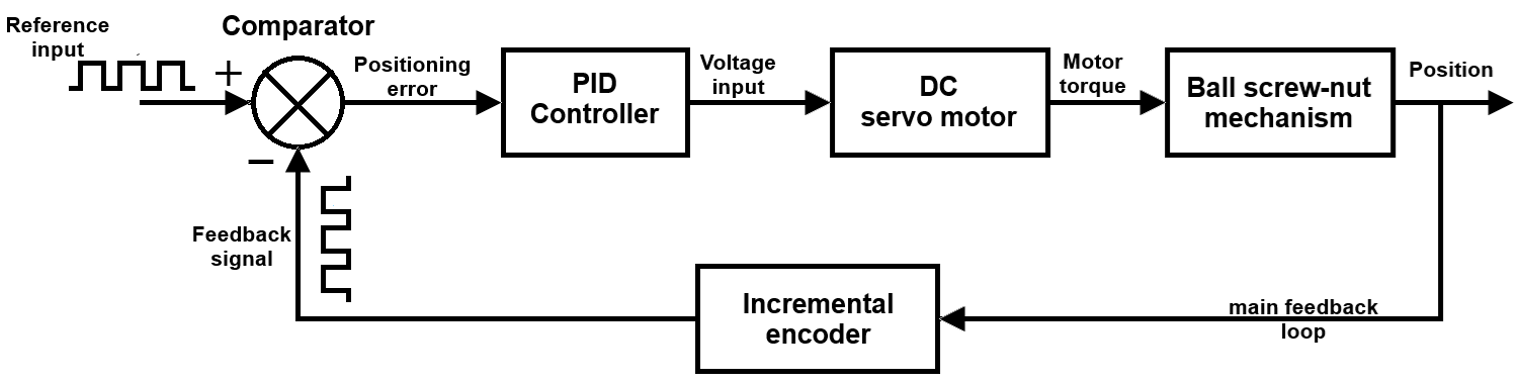
4.1. Modeling the Feed Drive Systems

The feed systems on the three axes of motion (X, Y, and Z) were modeled as closed-loop motion control systems, using the DC servo motor as the actuation device and the incremental encoder as the feedback device. A ball screw−nut mechanism was used as the transmission element. A block diagram of the system is shown in Figure 2.

It should be noted that although all three feed axes (X, Y, and Z) were numerically controlled, at this stage, the machine was a 2.5D machine. This meant that while the X- and Y-axes could perform simultaneous movements (in contouring mode), the Z-axis could only operate in single-axis mode. (It could not operate simultaneously with either the X- or Y-axis.) This was because the Z-axis drive system, including the servo motor and ball screw, was different from the X- and Y-axes systems.

Normally, the mathematical modeling of such a system is based on the transfer function in the relation below, considering the voltage applied on the armature as the input signal and the angular velocity of the motor as the output signal, which can be expressed as:

$${\displaystyle \frac{{\mathsf{\Omega }}_m\left(s\right)}{U\left(s\right)}}={\displaystyle \frac{K_t}{(J_{red}s+B_{red})(Ls+R)+K_t{K}_v}}.$$

(1)

The notations employed in the aforementioned relation were defined as follows:

-

Voltage applied to the armature) u [V] (the term U(s) represents the Laplace transform of the voltage input);

-

Angular speed of the motor shaft ωm [rad/s] (the term Ωm (s) represents the Laplace transform of the angular speed output;

-

Armature moment of inertia J_m [kgm²];

-

Coefficient of viscous friction B_m [Nms/rad];

-

Back electromotive force (emf) voltage constant K_v [V/rad/s];

-

Electromagnetic torque constant K_t [Nm/A];

-

Armature resistance R [Ω];

-

Armature inductance L [H].

In order to take into account all components of the motion control system, not just the motor, it was necessary to modify the above transfer function by relating the inertia and friction of moving parts other than the motor to the motor shaft. This was achieved by substituting J_m and B_m with J_red and B_red, respectively. This substitution signified reductions in the moment of inertia and viscous friction constant at the motor shaft. It is important to note that the ball screw was the sole rotating moving element considered in this system, with the coupling between the motor and the ball screw being negligible.

The values for J_red and B_red were calculated using the following relations:

$$J_{red}=J_m+{\displaystyle \frac{J_s}{i^2}}.$$

(2)

$$B_{red}=B_m+{\displaystyle \frac{B_s}{i^2}}.$$

(3)

The notations employed in Equations (2) and (3) are defined as follows:

-

Reduced moment of inertia at the motor shaft J_m [kgm²];

-

Coefficient of viscous friction reduced at the motor shaft B_red [Nms/rad];

-

Transfer ratio of the transmission between motor and screw i.

Since the motor and the lead screw were coupled directly, i = 1; therefore, Equations (2) and (3) can be rewritten as:

$$J_{red}=J_m+J_s.$$

(4)

$$B_{red}=B_m.$$

(5)

Finally, the transfer function between the voltage applied on the armature as the input signal and the angular velocity of the motor as the output signal can be expressed as:

$${\displaystyle \frac{\mathsf{\Omega }\left(s\right)}{U\left(s\right)}}={\displaystyle \frac{K_t}{(J_{red}s+B_{red})(Ls+R)+K_t{K}_v}}.$$

(6)

where Ω(s) is the Laplace transform of the angular velocity of the motor shaft input.

The simulation study of such systems characterized by transfer functions is usually performed in Simulink using specific blocks. This type of simulation is based on the representation of systems by equations and mathematical relations.

In this study, an alternative approach to simulation studies was adopted, utilizing the Simscape software (MATLAB v. 2016–v. 2024) module. The simulation was based on the physical phenomena occurring in the system, as opposed to the previous approach of using mathematical equations and relationships. The conventional transfer function blocks were substituted by blocks that emulated the behavior of physical systems, such as the “DC motor” block. The diagram for the simulation of an X-axis motion control system realized in Simscape is shown in Figure 3.

The feed drive system for the X- and Y-axes was characterized by the parameters shown in

Table 2. Parameters of the motion control system (X- and Y-axes).

Parameter	Meaning	Values (for X- and Y-Axes)
Mmn	Nominal torque developed by the motor	0.14 Nm
Kt	Electromagnetic torque constant	0.06 Nm/A
Kv	Back electromotive voltage constant	0.06 Vs/rad
Bm	Coefficient of viscous friction of the motor	0 Nms/rad
L	Armature inductance	0.029 H
R	Armature resistance	1.33 Ohm
Jm	Armature moment of inertia	0.00004 kgm2.
ps	Pitch of the lead screw	0.006 m
d	Ball screw diameter	0.01 m
L	Ball screw length	0.15 m
ρ	Screw material density (steel)	7800 kg/m3
Js	Lead screw moment of inertia	1.1486∙10−6 kgm2
Jred	Reduced moment of inertia at the motor shaft	4.1149∙10−5 kgm2
m	Overall mass of the system	m = 20 kg

.

4.2. System Dynamics

The control strategy used for the motion control systems involved the use of PID controllers.

One of the main objectives of the research was to provide users with a practical, cost-effective control solution for an open-architecture CNC equipment.

The classical PID controller was found to fulfill these requirements. As experimental research has shown, acceptable results have been obtained using this type of controller.

Also, industrial practice indicates that even in commercial industrial CNC industrial equipment, the classical PID control algorithm is the most widely used. Even if in the settings of such equipment there is a possibility to activate more advanced control facilities (e.g., feed-forward algorithms), these are often not activated.

The numerical implementation of a more advanced PID algorithm would have required more computational power than what is available on Arduino development boards, which are fitted with only 8-bit microcontrollers.

It should be kept in mind here that the Arduino boards need to run both the PID controller algorithm and handle the input quantities generated by the linear or circular interpolation algorithm.

Since the actual system is controlled numerically, the numerical form of the transfer function, shown in the equation below, was used for the PID controller:

$$H_{PID}\left(z\right)=K_P+K_I{T}_s{\displaystyle \frac{1}{z-1}}+K_D{\displaystyle \frac{N}{1+N{T}_s\frac{1}{z-1}}}.$$

(7)

where:

K_P is the proportional constant;

K_I is the integration constant;

K_D is the derivative constant;

T_s is the sampling time of the system.

The interactive “Tune” facility, available for the “PID Controller” block in Simulink, was used to tune the controller. It is imperative to consider that in the context of automatic position or displacement feedback systems, the overshoot should ideally be zero, or as close to this value as possible. Additionally, the physical limits of variation of the controller parameters for the experimental system must be taken into account. Preliminary experimental tests established that for the proportionality constant K_p, the limit was 200, and for the derivative constant K_D, the limit was 1. No limit was established for the integration constant K_I.

For the preliminary tuning of the controller using the specific tuning interface in MATLAB/Simulink, the control objective pursued a balanced approach between reference tracking (which would result in a better contouring accuracy of the CNC equipment) and input disturbance rejection (which would lead to a high robustness of the system to the action of technological resistive forces due to the machining process).

Figure 4 shows some forms of the step response and the values of the controller parameters for which they were obtained.

A summary of the PID controller parameter values, as well as system characteristics (rise time, settling time, overshoot) for the step responses shown in Figure 4a–d, is presented in

Table 3. Parameters of the controller and system characteristics.

Step Response	Controller Parameters	System Characteristics
Figure 4a	KP = 367.9, KI = 18.73, KD = −20.25, N = 12.12	Rise time = 0.155 s Settling time = 1.03 s Overshoot = 6.24%
Figure 4b	KP = 255.6, KI = 8.604, D = −24.94, N = 8.05	Rise time = 0.334 s Settling time = 1.06 s Overshoot = 4.4%
Figure 4c	KP = 357.3, KI = 17, KD = −30.36, N = 11.58	Rise time = 0.16 s Settling time = 0.768 s Overshoot = 12.2%
Figure 4d	KP = 155.2, KI = 3.294, KD = −17.59, N = 8.717	Rise time = 0.561 s Settling time = 0.966 s Overshoot = 0.938%

.

At this stage of studying the motion control system, the following can be stated:

-

It was determined that acceptable behavior was obtained for values of the proportional constant K_P of approximately 150;

-

The integral constant K_I exerted a relatively minor influence on the behavior of the system; that is to say, the smaller the integration constant, the better the system’s behavior;

-

Furthermore, it was not possible to draw any useful conclusions about the influence of the derivative constant and the filter coefficient N. The practical implementation of the effect of the derivative in the operation of the experimental system differed from the implementation used in the interactive tuning interface in Simulink.

In order to ensure the fidelity of the simulation process, a modified transfer function of the numerical PID controller was employed, thereby ensuring the simulation’s proximity to the behavior of the real system:

$$H_{PID}\left(z\right)=K_P+K_I{\displaystyle \frac{T_s}{z-1}}+K_D{\displaystyle \frac{z-1}{T_{s}z}}$$

(8)

To implement this form of transfer function, the Simulink blocks shown in Figure 5a were used. The “Saturation” block with ±24 V voltage limits from the simulation diagram, just after the PID controller subsystem, was also noticeable (also shown in Figure 3).

4.3. Positioning Regime

For single-axis rapid positioning, the motions of the moving elements of the system were usually along a trapezoidal velocity profile that included an acceleration phase, a constant-velocity phase, and a deceleration phase, as shown in Figure 6.

The notations employed in Figure 6 were defined as follows:

v_max is the maximum speed during the positioning cycle;

t_a is the duration of the acceleration phase;

t_ct is the duration of the constant speed travel phase;

t_d is the duration of the deceleration phase;

T is the total positioning cycle time.

The value of the parameters used to simulate the behavior of the system during the positioning regime are presented in

Table 4. Parameters of the positioning regime.

Parameter	Values
vmax	0.0083 m/s (500 mm/min)
ta	0.0167 s
tct	4.8 s
td	0.0167 s
T	4.8333 s
KP	140
KI	0
KD	0.05
Ts	0.0028 s

.

Figure 7 shows the comparative evolution of the imposed and actual speeds. It can be seen that the actual velocity followed the imposed velocity relatively closely, and most importantly, the maximum imposed value was reached. The shape of the variation of the effective velocity also ensured that jerking was avoided.

Figure 8 shows the comparative evolution of the imposed and actual positions. It can be seen that there was a difference in the time axis between the two positions, but it should be noted that this was only an instantaneous deviation and not a real positioning error. The fact that in the end, the two positions, imposed and actual, coincided shows that the positioning was carried out without error.

Another feature of the motion control system that could be studied by simulation in this case was its behavior in the presence of disturbances. In the simulations presented so far, the value of the disturbance torque was assumed to be zero, with only the resisting torque due to the load drive (the rotating or translating masses driven by the axis drive servo motor) acting in the system.

Figure 9a–c shows the evolution of the effective velocity for three values of the disturbance torque, 1% (0.0014 Nm), 2% (0.0028 Nm), and 5% (0.007 Nm), respectively, of the nominal torque developed by the axis drive servo motor (0.14 Nm).

It can be seen that in all three cases, although the resistant torque disturbance had a significant effect on the way in which the effective velocity varied, the system was eventually able to cancel its effect.

To determine whether the disturbance also affected the positioning accuracy, the evolution of the actual position in the presence of a resistive torque disturbance equal to 5% of the rated motor torque was plotted in Figure 9d.

From Figure 9d, it can be seen that the time evolution of the position signal was apparently insignificantly affected by the occurrence of the disturbance, but the final position value was different from the imposed value, x_imp = 40.1 mm = 0.0401 m, so there was a positioning error in this case. The amount of positioning error in this case was also very large for such a system, but it must also be taken into account that the disturbance torque was very large.

In conclusion, it can be stated that in the positioning regime, the system demonstrated an adequate level of resilience to disturbances that did not exceed 2% of the nominal torque developed by the motor. However, when this threshold was exceeded, the system’s performance was found to be less optimal.

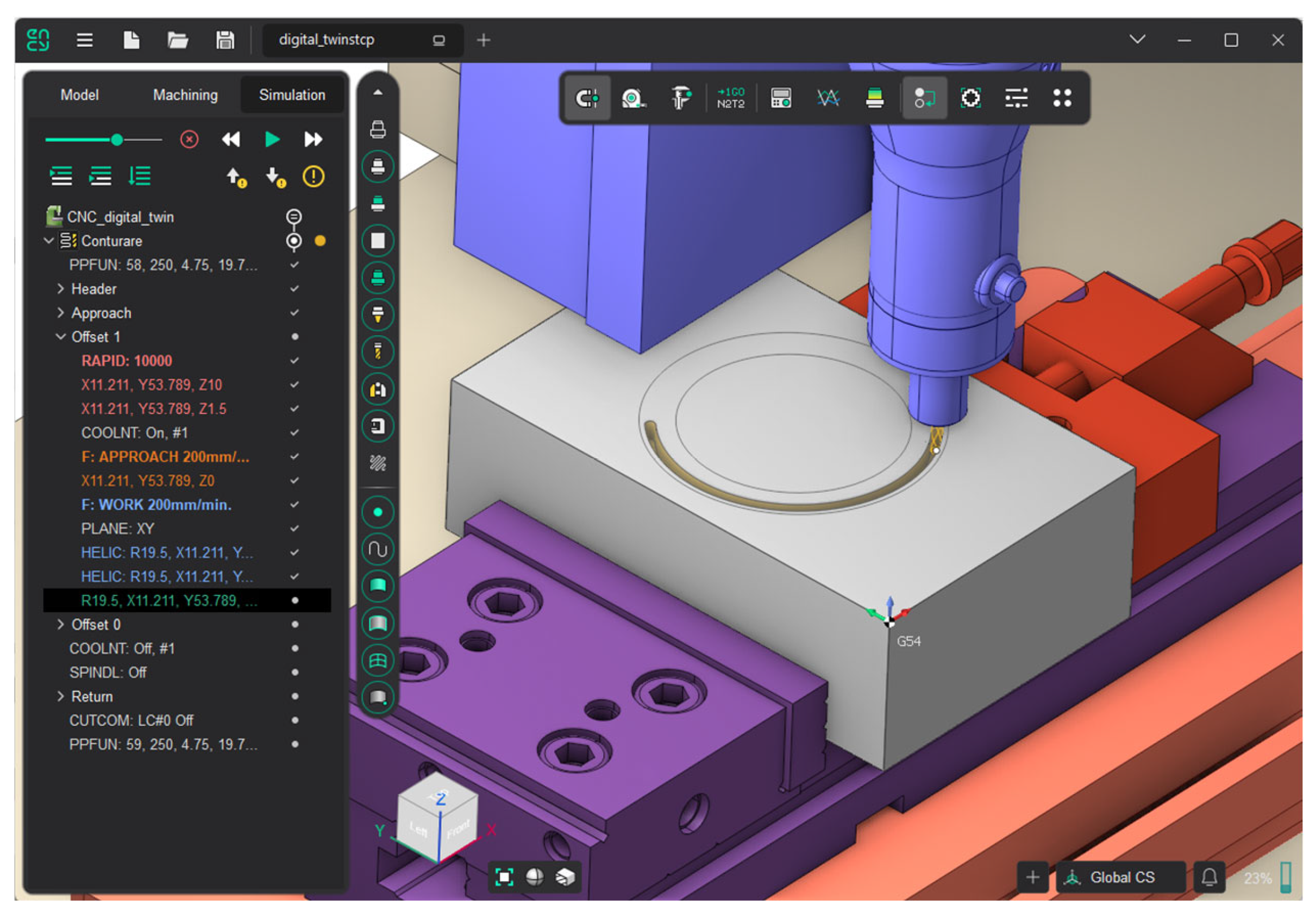
4.4. Contouring Regime and Circular Interpolation

The basic principle of motion control on CNC machines, from the point of view of generating the trajectories along which the tool must move, is as follows: each trajectory, regardless of its complexity, is broken down into straight line segments and circular arcs.

Similarly, in the case of translational movements, regardless of the number of numerical control axes available on the CNC, the trajectories are usually generated by combining the movements of two translational axes, in the XY, XZ, and YZ planes. Although it is theoretically possible, the displacement obtained by combining movements on three axes simultaneously is very rarely used in practice.

The movement mode in which simultaneous movements on several axes take place and machining operations (cutting) are performed during these movements is called the contouring mode. As mentioned above, a contour in a plane (the XY plane for the case study) is generated by decomposing it into entities, such as line segments and circular arcs.

There are two categories of interpolation algorithms, depending on the elementary trajectory generated, line segment or arc, linear interpolation algorithms, and circular interpolation algorithms. Even within these two categories, there are several types of algorithms. In the following, the construction of a simulation diagram will be pursued to allow the study by simulation of the contouring regime in general, with particularization on circular interpolation.

On the basis of the studies presented in [29,30], considering the coordinates x(t) and y(t) of a point on the circular arc, the relations can be written as:

$$\left\{\begin{array}{c}x\left(t\right)=R\left[K_{1}sin\right(f·t+\phi )-K_2\mathit{sin}(f·t)]\\ y\left(t\right)=R\left[K_{1}sin\right(f·t)+K_2\mathit{sin}(f·t+\phi )]\end{array}\right..$$

(9)

where:

R is the radius of the circle [m];

f is the sine function frequency [Hz]

φ is the sine function phase [rad];

K₁ and K₂ are constants to be specified later.

Further relations can be written as:

$$v=\omega ·R={\displaystyle \frac{2\pi }{T}}·R.$$

(10)

where:

v is the feed speed on the circular trajectory (constant) [m/s];

T is the time to generate a full circle (period) [s].

ω is the angular velocity [rad/s].

Also, it can be stated that:

$$T=n·T_s.$$

(11)

where:

Ts is the sampling period [s];

N is the total number of samples.

Combining relations (10) and (11), the total number of samples can be calculated as:

$$n={\displaystyle \frac{2\pi ·R}{v·T_s}}.$$

(12)

The smallest value of the angular displacement on the axis (angular increment) α_incr can be calculated with the following relation:

$${\alpha }_{incr}={\displaystyle \frac{2\pi }{T}}·T_s={\displaystyle \frac{v}{R}}·T_s.$$

(13)

Also, the smallest value of the linear displacement (linear displacement increment) l_incr can be calculated with the following relation:

$$l_{incr}=2R·{\displaystyle \frac{{\alpha }_{incr}}{2\pi }}={\displaystyle \frac{v}{\pi }}{T}_s.$$

(14)

Since the sine function used and the interpolation algorithm, respectively, have a numerical character, the relations can be written further as:

$$f={\displaystyle \frac{2\pi }{N{T}_s}}.$$

(15)

where:

N is the number of samples per period.

For N, the relation can also be written as:

$$N=round\left(n\right).$$

(16)

where round is a MATLAB function that rounds the bracketed value to the nearest integer.

Also, to preserve the numeric character of the sine function, the number of offset samples N_off can be defined as:

$$N_{off}={\displaystyle \frac{\phi N}{2\pi }}.$$

(17)

Since for this algorithm, the phase ρ is equal to π/2, one can rewrite the relation (17) as follows:

$$N_{off}={\displaystyle \frac{-\frac{\pi }{2}round\left(n\right)}{2\pi }}.$$

(18)

The relation (9) can now be rewritten as follows:

$$\left\{\begin{array}{c}x\left(t\right)=R\left[K_{1}sin\right({\displaystyle \frac{2\pi }{round\left(n\right)T_s}}·t-{\displaystyle \frac{\pi }{2}})-K_2\mathit{sin}({\displaystyle \frac{2\pi }{round\left(n\right)T_s}}·t)]\\ y\left(t\right)=R\left[K_{1}sin\right({\displaystyle \frac{2\pi }{round\left(n\right)T_s}}·t)+K_2\mathit{sin}({\displaystyle \frac{2\pi }{round\left(n\right)T_s}}·t-{\displaystyle \frac{\pi }{2}})]\end{array}\right..$$

(19)

For K₁ and K₂, the relations can be written as:

$$K_1=\mathit{cos}{\alpha }_{incr}\mathrm{and} K_2=\mathit{sin}{\alpha }_{incr}.$$

(20)

The smallest value of the angular displacement on the axis (angular increment), α_incr, can be calculated as a function of the total number of pulses emitted by the incremental numerical encoder of the displacement control system at one complete rotation, N_imp:

$${\alpha }_{incr}={\displaystyle \frac{360^0}{N_{imp}}}={\displaystyle \frac{360^0}{2024}}=0.1758^0.$$

(21)

For the smallest value of the linear displacement (linear displacement increment) l_incr, the relation can be written as:

$$l_{incr}={\displaystyle \frac{{\alpha }_{incr}·p_{sb}}{360^0}}={\displaystyle \frac{0.17{58}^0·6·10^{-3}}{360^0}}=2.92·10^{-6}\hspace{0.33em}m=2.92\hspace{0.33em}\mathsf{\mu }\mathrm{m}.$$

(22)

Knowing the value of l_incr and using the relation (14), one can calculate the value of the sampling period Ts for a trajectory forward velocity v = 0.0033 m/s as follows:

$$T_s={\displaystyle \frac{l_{incr}\pi }{v}}={\displaystyle \frac{\mathrm{2,92}·10^{-6}·\pi }{0.0033}}=0.0028\hspace{0.33em}\mathrm{s}.$$

(23)

Figure 10 shows the diagram used to simulate the behavior of the system under the circular interpolation regime.

The simulations aimed to study the behavior of the equipment when generating a full circle in the XY plane. In addition to the data calculated above, the following numerical values were used (

Table 5. Parameters used for circular interpolation simulation.

Parameter	Meaning	Values (for X- and Y-Axes)
R	Circle radius	0.030 m (30 mm)
v	Feed velocity	0.0033 m/s (198 mm/min)
K1	Constant	1
K2	Constant	3.068 · 10−4
C1	Initial position compensation constant	0.03 m (R)
C2	Initial position compensation constant	0
T	Generation period of a full circle	56.5487 s
n	Total number of samples at full-circle generation	20,480
N	Total number of samples during the period of generating a full circle	20,480

).

Figure 11a,b shows the comparative evolution of the imposed and actual position signals on the X- and Y-axes.

Figure 11c shows the full-circle, imposed, and effective trajectories obtained by simulation under zero technological resistant torques (dry-run). It can be seen that at the scale used in the figure, the two trajectories were practically superimposed.

In Figure 11d, which shows a scaled detail of Figure 11c, it can be seen that there were, however, some contouring deviations in the X-axis and Y-axis, which, according to the figure, were less than 0.05 mm, which is an acceptable value for the role and purpose of the proposed system.

Figure 12a shows the full-circle, imposed, and effective trajectories obtained by simulation, under conditions of technological resistant torques equal to 2% of the value of the nominal torques developed by the axis actuating servo motors (0.0028 Nm), acting on each axis.

From Figure 12a, it is relatively easy to notice the occurrence of path deviations, even with the naked eye, especially on the sectors of the circle located in quadrants I and IV. Figure 12b shows a scaled detail of Figure 12a, which highlights the occurrence of deviations between the imposed and actual paths that exceeded 1 mm.

Obviously, for a CNC system, deviations of more than 1 mm are large, but the following aspects should be taken into account

-

The proposed CNC equipment was a development system with open architecture, dedicated to the study of modular control solutions;

-

The size and rigidity of the equipment were relatively small, compared to industrial equipment, which, to some extent, explains the significant influence of the technological resistance moments on the contouring accuracy.

In the experimental program, measures to reduce the number of deviations between the imposed and the actual trajectory were aimed at reducing the number of these technological resistant moments using an appropriate choice of cutting regime parameters.

In practical terms, the aim was not to optimize the behavior of the CNC equipment but to rigorously determine the conditions under which it can be used as technological equipment for machining, its limits in terms of shape accuracy, and methods of reducing errors.

4.5. Physical Implementation of the System

The physical implementation of the open-control architecture CNC equipment (built by the authors) is illustrated in Figure 13a–c.

The notations in Figure 11a–c represent the following:

• The Y-axis incremental encoder;
• Y-axis DC servo motor (Dunkermotoren);
• X-axis DC servo motor (Dunkermotoren);
• X-axis incremental encoder;
• Z-axis DC servo motor (Pololu);
• Main spindle unit;
• Support structure (frame);
• Z-axis ball screw transmission unit;
• Workpiece fixing system;
• Y-axis ball screw transmission unit;
• X-axis ball screw transmission unit;
• Arduino control boards together with DC motor power supply boards.

The system was realized in a modular form and consisted of the following modules:

-

A supporting structure composed of extruded aluminum profiles;

-

Kinematic feed kinematic chains on the X-, Y-, and Z-axes, structured as closed-loop motion control systems. The drive equipment was the DC servo motor, and the feedback device was the incremental encoder. For the X- and Y-axes, Dunkermotoren GR63x25 servo motors (Dunkermotoren GmbH, Bonndorf, Germany)were employed, while a Pololu servo motor (Pololu, Las Vegas, USA) was utilized for the Z-axis. THK LM Guide Actuator (THK Co., Ltd., Tokyo, Japan) KR ball screw–nut type THK LM Guide Actuator KR were used as transmission devices on all three axes.

-

Main kinematic chain (main spindle drive unit) achieved through the integration of a Proxxon mini drilling machine, comprising a drive system powered by a single-phase AC motor with manual speed adjustment capability and a chuck-type tool clamping system for the cutting tool. This system enabled the manual clamping and replacement of cutting tools, including cylindrical mill, center drill, twist drill, and tapping drill types. The working unit provided the primary cutting motion for the CNC system.

-

Command and control module achieved through the implementation of two Arduino MEGA development boards, each equipped with an 8-bit AVR ATMega 2560 microcontroller (Microchip Technology, Chandler, AZ, USA). The Arduino boards were responsible for issuing commands to the drive modules of the three axes (as reference inputs for the automatic motion control systems) and to the main spindle module. The term “control” in this context refers to the implementation of PID-type automatic control algorithms on each motion axis. The utilization of these command-and-control systems guaranteed the system’s open-architecture nature, facilitating the implementation of flexible control algorithms and the straightforward modification of control parameters. The command-and-control module incorporated Pololu Dual VNH5019 boards (drivers, Pololu, Las Vegas, USA), which facilitated the power supply for DC servo motors, with voltages ranging from 5.5–24 V and currents ranging from 12–24 A. Each of these two drivers was capable of powering up to two DC servo motors and was compatible with Arduino MEGA boards (Arduino S.R.L., Monza, Italy).

It is imperative to reiterate that the two Arduino MEGA boards facilitated the coordination and control of all three drive modules, as well as the main spindle module.

5. Developing a Digital Twin of the System

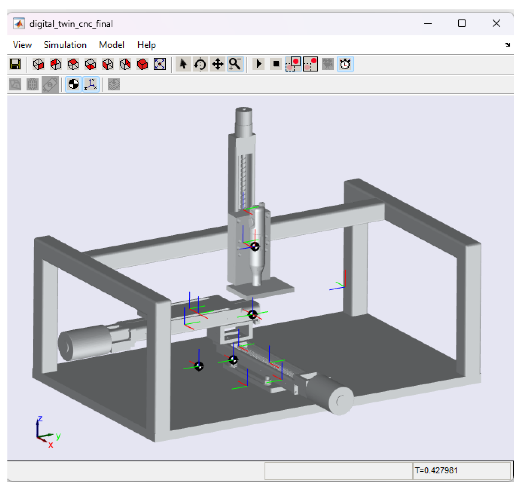
5.1. CAE Simulation

The process of creating a digital twin for CNC equipment entailed the sequence of steps illustrated in Figure 14.

The steps shown in Figure 13 are detailed below.

Realizing the 3D model of the CNC equipment as an assembly in Solidworks

The first step required making a 3D model of the CNC equipment in a CAD program. The Solidworks software (v. 2019) package was chosen for this task.

The use of the Solidworks software package to realize the 3D model as an assembly, later broken down into functional modules, was necessary because it was directly integrated with MATLAB and Simulink, allowing the automatic generation of a kinematic model in the latter by exporting the 3D assembly from Solidworks.

Separating the assembly into functional modules

The separation into subassemblies of the CNC equipment assembly was necessary in order to correctly identify its functional modules in the export process from Solidworks to MATLAB/Simulink. The identification of movable components (feed axes, main spindle unit) and fixed components (frame, fixtures) was performed by defining the corresponding constraints in Solidworks (v. 2019). Figure 15 shows the 3D model of the CNC equipment together with the functional modules.

Exporting the assembly module by module from Solidworks to MATLAB/Simulink

The Solidworks interface includes specific commands for managing the export of assemblies to MATLAB/Simulink.

To export the 3D model from Solidworks, we went to the main menu Tools, submenu Simscape Multibody Link, submenu Export, and command Simscape Multibody.

These commands generated a file with the .xml extension to be imported into the MATLAB workspace with the command:

smimport(‘filename’)

(24)

The import generated a Simulink file (slx file) and a data file (m file).

The slx file included all the necessary information for the kinematic simulation of the modeled CNC equipment using Simulink and its modules Simscape Multibody or Simscape Multibody First Generation (Simmechanics), depending on the MATLAB version used.

Completing the Simulink diagram with kinematic joint actuation systems and reference input generation systems

At this stage the diagram could only simulate the motions executed by the CNC equipment, but only in an uncontrolled way. By supplementing the diagram with kinematic joint actuation systems and reference frame generation systems, the diagram in Figure 15 was obtained, which allowed the simulation of the system behavior both kinematically and dynamically.

Kinematic simulation, in this case, means the possibility to generate the kinematic reference quantities, either in a positioning or in a circular interpolation regime, and to study how they are processed in the system from input to output.

The dynamic simulation allowed the evaluation of how motion control systems influenced the behavior of the CNC equipment and how the technological resisting forces acting at the level of the main spindle influenced the operation of the X- and Y-axes feed systems.

Most of the component subsystems of the diagram in Figure 15 were already presented in the previous figures, as follows:

-

The axis drive system (X, Y, Z) was presented in Figure 2;

-

The PID controller was presented in Figure 5a;

-

The input variable generation system (X, Y) was presented in Figure 2 or Figure 10, depending on the operating mode (fast positioning or contouring).

The diagram in Figure 16 made it possible to simulate the movements of the CNC equipment, but this simulation was complex: on the one hand, the laws of motion describing the displacements of the moving elements (in different working regimes, either rapid positioning or plane contouring) were introduced; on the other hand, the diagram made it possible to study the effects caused by the dynamics of the drive systems for each axis on the movements. The diagram also made it possible to study the effects of changing the parameters of the PID controllers on the behavior of the system for each axis. It also made it possible to study the effects of technological resisting forces and moments, which can be introduced either as quantities that vary according to a certain law of variation with time (at the top level of the diagram, using the technological resistance force signal generation subsystems) or as constant quantities that vary stepwise (using the disturbance torque-type blocks in the axis drive subsystems).

Figure 17 shows a screenshot of the system motion simulation in the Mechanics Explorer interface.

The last step from Figure 14, integrating machining process simulation into the digital twin system, is explained in the next section.

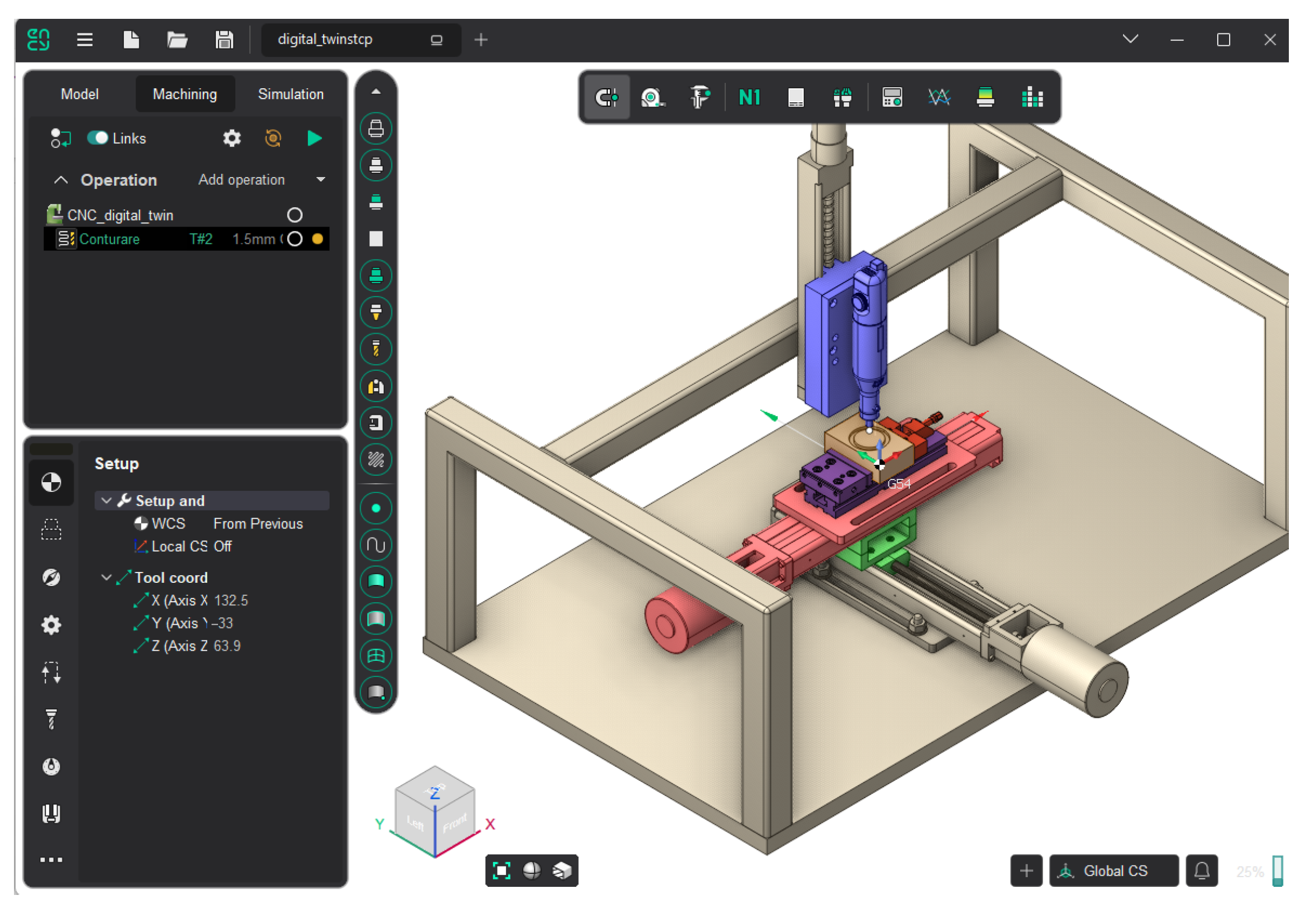
5.2. CAM Simulation

In order for the integrated digital twin simulation system to also allow CAM simulation, a kinematic model of the CNC equipment was created using the MachineMaker module of the CAM ENCY software (v. 1) package.

Figure 18 shows a screenshot of MachineMaker showing how the components of the kinematic model of the CNC equipment were defined.

Once the kinematic model was created, it was used to simulate machining in the CAM ENCY program. Figure 19 and Figure 20 show screenshots from this program showing how the workpiece was clamped on the machine table and the simulation of a milling operation.

It should be noted that the simulation process was a complete one, simulating the movements performed by the tool, those performed by the workpiece, and those performed by the moving elements of the machine. It also simulated how the tools removed material from the workpiece during the milling process.

5.3. Features of the Integrated CAE/CAM Digital Twin Simulation Environment

The previous sections described the steps taken to develop the integrated digital twin simulation system.

Table 6. Facilities offered by the integrated digital twin simulation environment.

Simulation Type	Objective	What Can Be Simulated/Studied	Benefits
CAE simulation	Study of the behavior of motion control systems in the structure of the CNC equipment	- Dynamic behavior of motion control systems in different operating regimes (fast positioning and contouring). - Influence of controller tuning parameters on positioning accuracy and contouring accuracy. - Determination of the required inputs (displacements, velocities, and accelerations). - Values of the quantities occurring in the system during its operation (voltages, currents, forces, moments, displacements, velocities, and accelerations). - Visualization of the movement of the moving parts of the equipment and how static and dynamic loads influence these movements.	Motion control system controllers can be tuned. Positioning accuracy can be improved. Contouring accuracy can be improved. Cutting regime can be designed according to the required machining accuracy. Dynamic overloading of the equipment can be avoided.
CAM simulation	Study of the movement of mobile elements of CNC equipment during the milling of workpieces	- How the blank is clamped to the table of the equipment (including the vise is simulated). - Movement of the cutting tool. - Movement of the workpiece. - Movement of the mobile parts of the equipment. - How the material is removed from the blank.	Collisions between tool and workpiece blanks can be identified and eliminated. Collisions between tool and fixtures (vice and/or flanges) can be identified and eliminated. Collisions between moving parts of the machine can be identified and eliminated. Overtravel on the axes of motion of the equipment can be identified. NC code for part machining can be generated and verified.

describes the capabilities it provided for simulating the behavior of the CNC equipment.

Summarizing the information in Table 6, it can be stated that the realized digital twin system can perform the following functions.

Virtual commissioning tool function

The proposed digital twin system allowed the study of the motions of the moving elements of the CNC equipment in both CAE (Mechanics Explorer interface) and CAM components. In the first case (CAE), dynamic simulations in different regimes were complemented by visual confirmation of whether or not the moving parts were moving (if the loads exceeded the allowed limits). In the second case (CAM), it was verified that the correlation of the simultaneous motions required for machining complex-shaped parts did not lead to collisions between the moving parts of the equipment or between the moving parts and tool/tool holders, workpieces, or fixtures of the workpieces.

Real-time dynamic modeling function

The correlation between the CAE and CAM components of the digital twin made up for the shortcomings of each component individually. Thus, the CAE simulation, while allowing real-time study of the system dynamics, did not allow a realistic visualization by simulation of the milling machining process. On the other hand, the CAM component, which allowed the visualization of the machining process, did not provide information related to the influence of the dynamic stresses occurring in the equipment and the tuning parameters on the machining accuracy.

Simulation-based design aid function

The digital twin system can also be used for the design (or redesign) of CNC equipment, especially if it is realized in the open-architecture version. Any structural design solution (or in the case of re-design, any constructive change) can be tested and validated by CAM simulation, while the CAE component allows testing and validation of changes in actuation and motion control systems in the feed drive kinematic chains.

At present, the interaction between the digital twin system and the CNC equipment is limited by the absence of an advanced sensor system to accurately measure the physical quantities occurring in the real system and to transfer this information to the digital twin for simulation testing.

The CAE and CAM components of the digital twin system are useful both as independent modules (as summarized in Table 6), but they can also exchange data between them, as shown in the following examples:

-

The NC numerical code generated by the CAM component (which describes the trajectories followed for machining a part) can be used to generate kinematic input quantities for the CAE model that are more complex than a simple circular in-plane trajectory;

-

The values of voltages, currents, and moments indicated by the CAE model can be used to design and test in the CAM model cutting regimes that do not lead to overstressing the CNC equipment.

6. Experimental Tests

As mentioned in the previous sections, the command and control of the system were realized using two Arduino MEGA boards, equipped with 8-bit AVR ATMega 2560 (Microchip Technology, Chandler, AZ, USA) (Figure 21a) and AVR ATMega 2560 microcontrollers, together with Pololu Dual VNH5019 (Pololu, Las Vegas, USA) (Figure 21b) boards, which provided the DC servo motors with voltages ranging from 5.5–24 V and currents ranging from 12–24 A.

The Pololu Dual VNH5019 VNH5019 Pololu Dual boards (acting as DC motor control drivers) were connected to both the Arduino development boards and the motors they control. As previously stated, the two Arduino MEGA boards, together with the two Pololu Dual VNH5019 boards, provided command and control for all three axis drive modules, as well as the main spindle module.

Incremental quadrature photoelectric digital transducers (encoders) were used to realize closed-loop control. The proposed resolution of the CNC system determined the number of pulses/rotation required. Thus, the Dunkermotoren encoder (which equips the motors) was used for the X- and Y-axes, with a resolution of 2048 pulses/rotation, and for the Z-axis, which, at this stage of the system development, was used only for positioning. There was the possibility of reading 64 pulses/rotation.

Some of the characteristics of the encoders used are shown below:

-

Resolution: 2048 pulses/rotation (X, Y), 64 pulses per rotation (Z);

-

Input voltage: 5–12 V, DC;

-

Maximum rotational speed: 6000 rpm;

-

Permissible radial load: 5 N;

-

Permissible axial load: 3 N;

-

Cable length: 50 cm;

-

Output shaft diameter: 6 mm.

The MATLAB–Simulink software package, together with the additional module dedicated to Arduino hardware-based systems, Simulink Support Package for Arduino Hardware, was used to control the X- and Y-axes motions of the proposed CNC system.

To ensure the real-time control of the X- and Y-axes movements, the diagram presented in Figure 22 was employed. This ensured the real-time generation and execution of the requisite executable code for the operation of the AVR ATMega 2560 microcontrollers.

The diagram used specific blocks from Simulink, as well as blocks from the Simulink Support Package for Arduino Hardware, which are explained in

Table 7. Main blocks from the Simulink Support Package for Arduino Hardware used in the structure of the simulation diagram in Figure 21.

Block	Block Name	Function
	Encoder	The Encoder block outputs the number of pulses from a quadrature encoder on a rotary motor connected to an Arduino board. Each increase in the number of encoder pulses indicates that the motor is rotating clockwise. Each decrease in the number of encoder pulses indicates that the motor is rotating counterclockwise. The total number of pulses represents the incremental position of the rotating motor.
	Digital Output	Sets the logic value of a digital pin on the Arduino board: - Transmitting value 1 to the block input sets the logic value of the HIGH digital pin to 5 V or 3.3 V, depending on the board voltage. - Transmitting value 0 to the block input sets the logic value of the LOW digital pin to 0 V.
	PWM	The PWM block generates variable duty-cycle rectangular pulses (width modulated) depending on the input value sent to the block on the Arduino board hardware terminal. This block allows a digital output to provide a range of different power levels, similar to that of an analog output.

.

The diagram in Figure 22 also used two “Numerical PID controller” subsystems of the type shown in Figure 3 and two “Reference position generation” subsystems of the type shown in Figure 9. The sampling period used for the real-time control system was T = 0.001 s.

Also used in the diagram in Figure 22 was the user function (introduced via a MATLAB Function block) “Speed”, which had the following syntax:

function [pin1, pin2, pwm] = fcn(speed)
pin1 = 1;
pin2 = 0;
if speed < 0
pin1 = 0;
pin2 = 1;
end
pwm = abs(sped);

(25)

Design of the Experiments

Simulations were carried out under varying working conditions, including feed rates, moving masses, and cutting forces, to adapt the tuning of the PID controllers process to the real behavior of the system. For each configuration, multiple PID sets were tested, either directly from autotuning or refined manually, based on the Ziegler–Nichols logic.

Each simulation output was evaluated using three quantitative indicators:

• Settling time (T_s);
• Steady-state error (E_ss);
• Maximum trajectory deviation (E_max).

Using a weighted objective function, the resulting performance data were aggregated:

$$J={\alpha }_1·T_s+{\alpha }_2·E_{ss}+{\alpha }_3·E_{max}$$

(26)

where α₁ = 0.4, α₂ = 0.4, and α₃ = 0.2, accentuating stability and the positional accuracy.

This concept allowed a balanced comparison between configurations, avoiding subjective or single-criterion selection. The configuration Kp = 140, Ki = 0, Kd = 0.05 achieved the lowest global score (J = 0.245). Excellent performance indicators were registered: settling time = 0.566 s, steady-state error = 0.025 mm, and maximum deviation = 0.183 mm. These values were consistent across both positioning and 2D circular interpolation regimes.

Although not based on a complete factorial design, the procedure reflected a practical applied statistical method. The process enabled not only the identification of the best-performing configuration in absolute terms but also an evaluation of trade-offs under different scenarios. Two final configurations—one PI and one full PID—were selected and implemented on the real CNC system. Subsequently, experimental tests, run under the same conditions as the simulations, were designed to test the predicted behavior.

Due to the limited stiffness of the system, soft materials were chosen for the experimental tests. The chosen material (NECURON 651, NECUMER GmbH, Bohmte, Germany) fell into this category and also had a good machining behavior. (The chips generated were discontinuous and did not affect the surface of the tool and/or the machined part.) This was important because the CNC equipment had no cooling or chip evacuation systems.

The tool clamping system also limited the maximum diameter of tools that could be mounted in the main spindle to 6 mm. It was decided to use a 1 mm diameter tool, both for reasons of low rigidity of the equipment and to limit the amount of chips generated, since, as mentioned above, there was no chip evacuation system.

To experimentally test the contouring accuracy of the proposed CNC system, a circular groove with an outside diameter of 31 mm and an inside diameter of 29 mm was machined, as shown in Figure 23a. A picture of a machined circular groove is shown in Figure 23b. The workpiece material was NECURON 651, a composite polymer and a mild material with a compressive strength of 25 N/mm².

A 1 mm diameter cylindrical end mill was used for machining. The center of the cutter described a circle with a diameter of 30 mm, exactly as in the simulation of the contouring regime. Two sets of controller parameters were used, the measurement of the inner and outer diameters of the flute was performed with the GOM Atos Core 200 optical measuring device, and the GOM Inspect Suite 2020 software package was used for data processing and visualization.

Figure 24 and Figure 25 show the results of measuring the inner and outer diameters of the circular groove for the two sets of controller parameters on the X- and Y-axes.

The first set of controller parameters was as determined from the simulation study, and a zero value of the derivative constant was used for the second set. This was tried in order to reduce the computational effort of the software system in real time and to study the influence of this on the processing accuracy.

It can be observed that the system had a dimensional accuracy that is typical of equipment in this category, which, of course, can still be improved, in particular by intervening on the mechanical structure to increase its rigidity. However, experimental tests showed that the system can work in contouring mode (simultaneous displacements on two axes, X and Y), and the hardware control system (Arduino boards) worked efficiently with the software control system (MATLAB–Simulink) implemented in real time.

An industrial CNC system designed for steel cutting in the machine-building industry typically exhibits deviations from the nominal dimensions of the circular paths in the order of hundredths of a millimeter, practically an order of magnitude smaller than the proposed system. On the other hand, however, the costs of such systems are much higher. (It can be estimated that they exceed the costs of the proposed system by up to 100 times.) Also, such high accuracies are often not necessary in industrial practice.

It can therefore be stated that the proposed system can be used in a wide range of applications for which lower accuracies (in the order of tenths of a millimeter) are acceptable and can be listed here as machining of injection molds for plastic packaging, machining of parts made of soft materials (mainly wood, but also other types of materials), engraving operations, and machining operations of parts for decorative purposes.

7. Conclusions

Within this paper, an experimental open-architecture CNC system was proposed and realized. An integrated digital twin CAE/CAM simulation environment was also developed for this system.

The CAE simulation part was implemented in MATLAB–Simulink–Simscape, where simulation diagrams were developed to study the behavior of the motion control systems in the structure of the CNC equipment under different working regimes (fast positioning and contouring in the XY plane). The CAM simulation part was implemented in the ENCY software package, where a kinematic model of the system was developed, which allowed the study of the motion of the moving elements of the CNC equipment during the milling machining of parts.

Experimental tests were also carried out to verify the efficiency of the multi-axis (X- and Y-axes) motion control systems, realized on the basis of Arduino MEGA development boards using the MATLAB–Simulink package as real-time control software. The experimental tests also validated the accuracy of the simulation studies in terms of tuning the numerical controllers.

Of course, the proposed system had limitations, among which the following can be listed:

-

The rigidity of the proposed equipment was relatively low, mainly also due to the small size of the structural elements;

-

The possibility of adapting control systems based on Arduino control boards to an equipment of increased size and rigidity (scalability) needs to be confirmed by further research;

-

The experimental tests were performed only on soft materials, which somewhat limited practical applications.

-

Future research directions to be addressed include:

-

Development of digital twins that also include software modules for processing information from sensors and transducers mounted on the physical system;

-

Implementation of more advanced control strategies than PID strategies on the developed CNC system (feed-forward controllers, fuzzy controllers, etc.) or even AI-based control strategies;

-

Use of more advanced microcontroller control cards (16 or 32 bit) as command-and-control systems for the developed CNC equipment;

-

Integration of sensor feedback for real-time correction;

-

Considering a wider range of workpiece materials.

References

- Papadopoulos, K.G.; Papastefanaki, E.N.; Margaris, N.I. Explicit analytical PID tuning rules for the design of type-III control loops. IEEE Trans. Ind. Electron. 2012, 60, 4650–4664. [Google Scholar] [CrossRef]
- Borase, R.P.; Maghade, D.K.; Sondkar, S.Y.; Pawar, S.N. A review of PID control, tuning methods and applications. Int. J. Dyn. Control 2021, 9, 818–827. [Google Scholar] [CrossRef]
- Díaz-Rodríguez, I.D.; Sangjin, H.; Bhattacharyya, S.P. Analytical Design of PID Controllers; Springer: Berlin/Heidelberg, Germany, 2019; ISBN 978-3-030-18227-4. [Google Scholar]
- Gai, H.; Li, X.; Jiao, F.; Cheng, X.; Yang, X.; Zheng, G. Application of a New Model Reference Adaptive Control Based on PID Control in CNC Machine Tools. Machines 2021, 9, 274. [Google Scholar] [CrossRef]
- Sun, X.; Liu, N.; Shen, R.; Wang, K.; Zhao, Z.; Sheng, X. Nonlinear PID Controller Parameters Optimization Using Improved Particle Swarm Optimization Algorithm for the CNC System. Appl. Sci. 2022, 12, 10269. [Google Scholar] [CrossRef]
- Yu, Z.; Liu, N.; Wang, K.; Sun, X.; Sheng, X. Design of Fuzzy PID Controller Based on Sparse Fuzzy Rule Base for CNC Machine Tools. Machines 2023, 11, 81. [Google Scholar] [CrossRef]
- Liu, L.; Xu, Z.; Qu, X. A Reconfigurable Architecture for Industrial Control Systems: Overview and Challenges. Machines 2024, 12, 793. [Google Scholar] [CrossRef]
- Latif, K.; Adam, A.; Yusof, Y.; Kadir, A.Z.A. A review of G code, STEP, STEP-NC, and open architecture control technologies based embedded CNC systems. Int. J. Adv. Manuf. Technol. 2021, 114, 2549–2566. [Google Scholar] [CrossRef]
- Zhou, X. An optimized data interaction structure for SERCOS-based open CNC system. Int. J. Adv. Manuf. Technol. 2023, 129, 4643–4661. [Google Scholar] [CrossRef]
- Liu, Q.; Liu, H.; Xiao, J.; Tian, W.; Ma, Y.; Li, B. Open-architecture of CNC system and mirror milling technology for a 5-axis hybrid robot. Robot. Comput.-Integr. Manuf. 2023, 81, 102504. [Google Scholar] [CrossRef]
- Dharmawardhana, M.; Ratnaweera, A.; Oancea, G. STEP-NC Compliant Intelligent CNC Milling Machine with an Open Architecture Controller. Appl. Sci. 2021, 11, 6223. [Google Scholar] [CrossRef]
- Attar, H.; Abu-Jassar, A.T.; Amer, A.; Lyashenko, V.; Yevsieiev, V.; Khosravi, M.R. Control system development and implementation of a CNC laser engraver for environmental use with remote imaging. Comput. Intell. Neurosci. 2022, 1, 9140156. [Google Scholar] [CrossRef]
- Khan, Z.H.; Rahman, T.; Arabi, S.; Mohammad, S.; Khan, M.M.; Dey, R.; Khan, M.M.; Mukherjee, D. Development of a Low-Cost CNC Machine Laser Engraver. In Proceedings of the 2021 IEEE 12th Annual Ubiquitous Computing, Electronics & Mobile Communication Conference (UEMCON), New York, NY, USA, 1–4 December 2021. [Google Scholar] [CrossRef]
- Das, U.C.; Shaik, N.B.; Suanpang, P.; Nath, R.C.; Mantrala, K.M.; Benjapolakul, W.; Gupta, M.; Somthawinpongsai, C.; Nanthaamornphong, A. Development of automatic CNC machine with versatile applications in art, design, and engineering. Array 2024, 24, 100369. [Google Scholar] [CrossRef]
- Cao, X.; Zhao, G.; Xiao, W. Digital Twin–oriented real-time cutting simulation for intelligent computer numerical control machining. Proc. Inst. Mech. Eng. Part B J. Eng. Manuf. 2022, 236, 5–15. [Google Scholar] [CrossRef]
- Yao, K.-C.; Chen, D.-C.; Pan, C.-H.; Lin, C.-L. The Development Trends of Computer Numerical Control (CNC) Machine Tool Technology. Mathematics 2024, 12, 1923. [Google Scholar] [CrossRef]
- Luo, W.; Hu, T.; Zhang, C.; Wei, Y. Digital twin for CNC machine tool: Modeling and using strategy. J. Ambient Intell. Humaniz. Comput. 2019, 10, 1129–1140. [Google Scholar] [CrossRef]
- Luo, W.; Hu, T.; Ye, Y.; Zhang, C.; Wei, Y. A hybrid predictive maintenance approach for CNC machine tool driven by Digital Twin. Robot. Comput.-Integr. Manuf. 2020, 65, 101974. [Google Scholar] [CrossRef]
- Tao, F.; Xiao, B.; Qi, Q.; Cheng, J.; Ji, P. Digital twin modeling. J. Manuf. Syst. 2022, 64, 372–389. [Google Scholar] [CrossRef]
- Heo, E.; Yoo, N. Numerical Control Machine Optimization Technologies through Analysis of Machining History Data Using Digital Twin. Appl. Sci. 2021, 11, 3259. [Google Scholar] [CrossRef]
- Pan, L.; Guo, X.; Luan, Y.; Wang, H. Design and realization of cutting simulation function of digital twin system of CNC machine tool. Procedia Comput. Sci. 2021, 183, 261–266. [Google Scholar] [CrossRef]
- Wei, Y.; Hu, T.; Zhou, T.; Ye, Y.; Luo, W. Consistency retention method for CNC machine tool digital twin model. J. Manuf. Syst. 2021, 58, 313–322. [Google Scholar] [CrossRef]
- Pantelidakis, M.; Mykoniatis, K. Extending the digital twin ecosystem: A real-time digital twin of a LinuxCNC-controlled subtractive manufacturing machine. J. Manuf. Syst. 2024, 74, 1057–1066. [Google Scholar] [CrossRef]
- Vishnu, V.S.; Varghese, K.G.; Gurumoorthy, B.J.P.C. A data-driven digital twin of CNC machining processes for predicting surface roughness. Procedia CIRP 2021, 104, 1065–1070. [Google Scholar] [CrossRef]
- Liu, K.; Song, L.; Han, W.; Cui, Y.; Wang, Y. Time-varying error prediction and compensation for movement axis of CNC machine tool based on digital twin. IEEE Trans. Ind. Inform. 2021, 18, 109–118. [Google Scholar] [CrossRef]
- Xue, R.; Zhang, P.; Huang, Z.; Wang, J. Digital twin-driven fault diagnosis for CNC machine tool. Int. J. Adv. Manuf. Technol. 2024, 131, 5457–5470. [Google Scholar] [CrossRef]
- Yang, X.; Ran, Y.; Zhang, G.; Wang, H.; Mu, Z.; Zhi, S. A digital twin-driven hybrid approach for the prediction of performance degradation in transmission unit of CNC machine tool. Robot. Comput.-Integr. Manuf. 2022, 73, 102230. [Google Scholar] [CrossRef]
- Yu, H.; Yu, D.; Wang, C.; Hu, Y.; Li, Y. Edge intelligence-driven digital twin of CNC system: Architecture and deployment. Robot. Comput.-Integr. Manuf. 2023, 79, 102418. [Google Scholar] [CrossRef]
- Masory, O.; Koren, Y. Reference-Word Circular Interpolators for CNC Systems. J. Eng. Ind. 1981, 104, 400–405. [Google Scholar] [CrossRef]
- Suh, S.-H.; Kang, S.K.; Chung, D.-H.; Stroud, I. Theory and Design of CNC Systems; Springer: London, UK, 2008. [Google Scholar]