


Controlling Product Properties in Forming Processes Using Reinforcement Learning—An Application to V-Die Bending

Abstract
1. Introduction
2. State of the Art
2.1. Die Bending
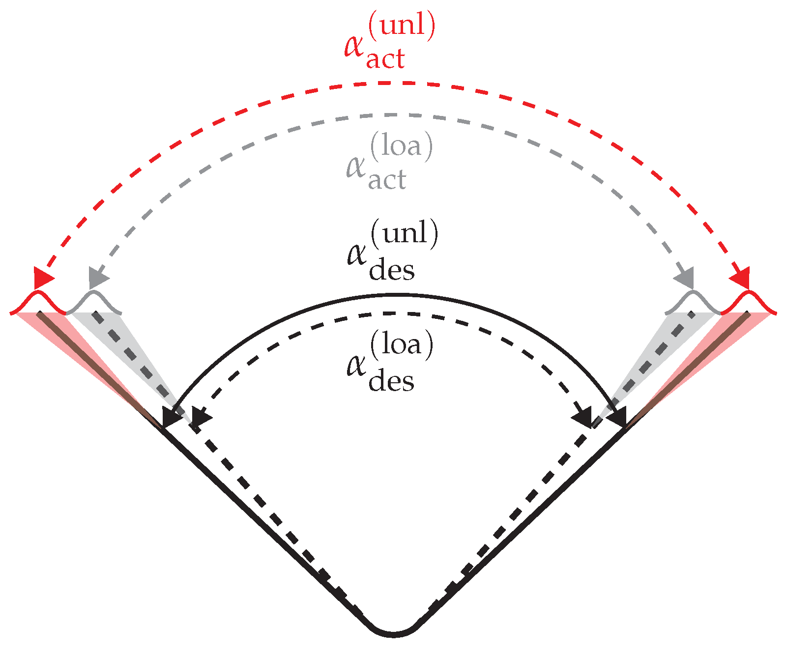
2.1.1. Springback
- : Desired bending angle after unloading the component;
- : Actual bending angle after unloading the component;
- : Desired bending angle with loaded component (in process);
- : Actual bending angle with loaded component (in process).
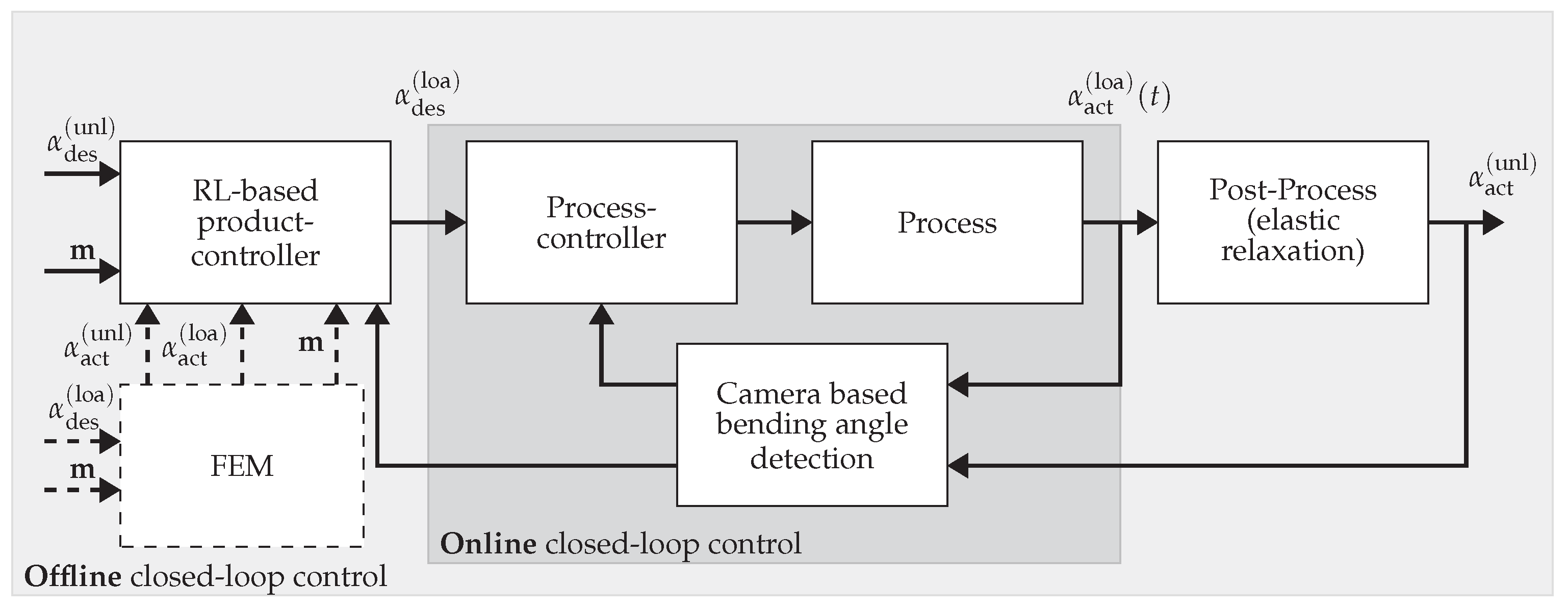
2.1.2. Control Approaches
2.2. Reinforcement Learning
2.2.1. Markov Decision Processes
2.2.2. Optimal Control
2.2.3. Actor-Critic Algorithms
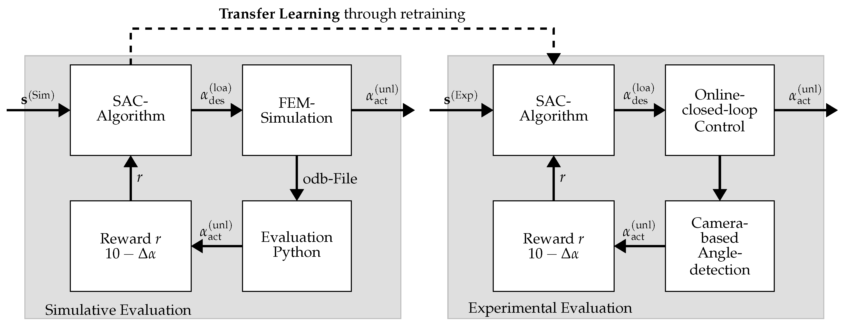
3. Methodology
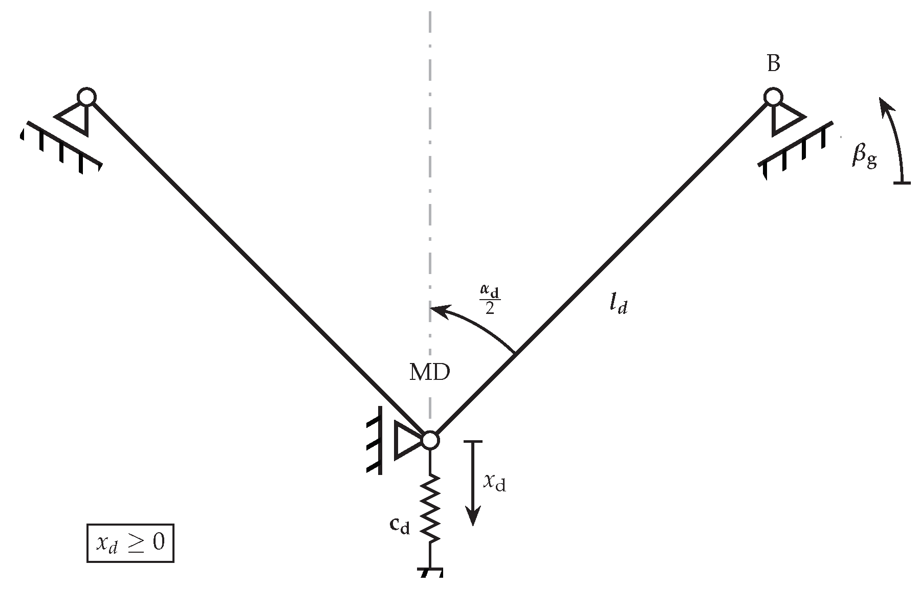
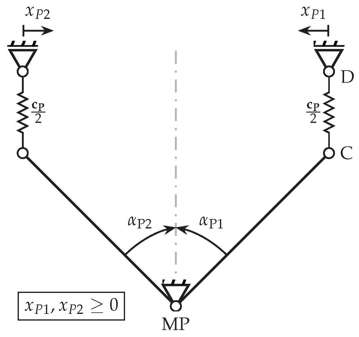
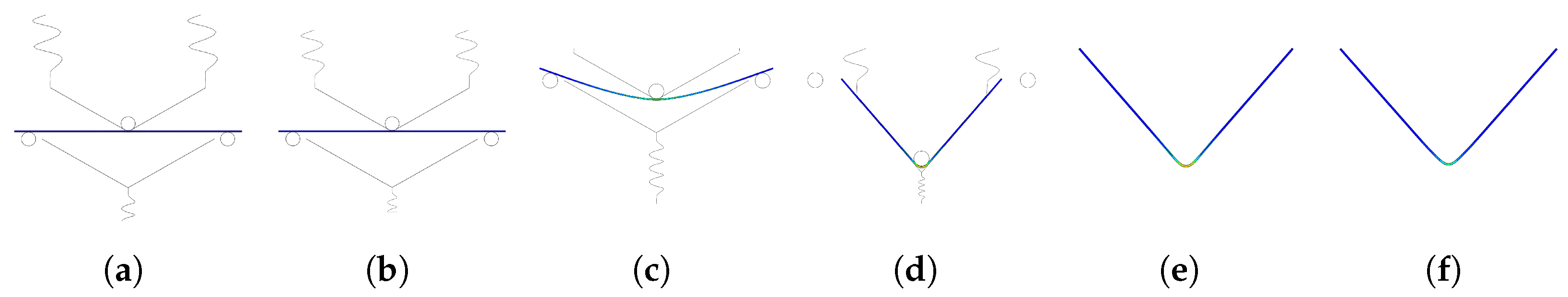
3.1. Design of Variable Die Bending Tool
3.2. Finite Element Simulation
3.3. Experimental Setup
4. Results
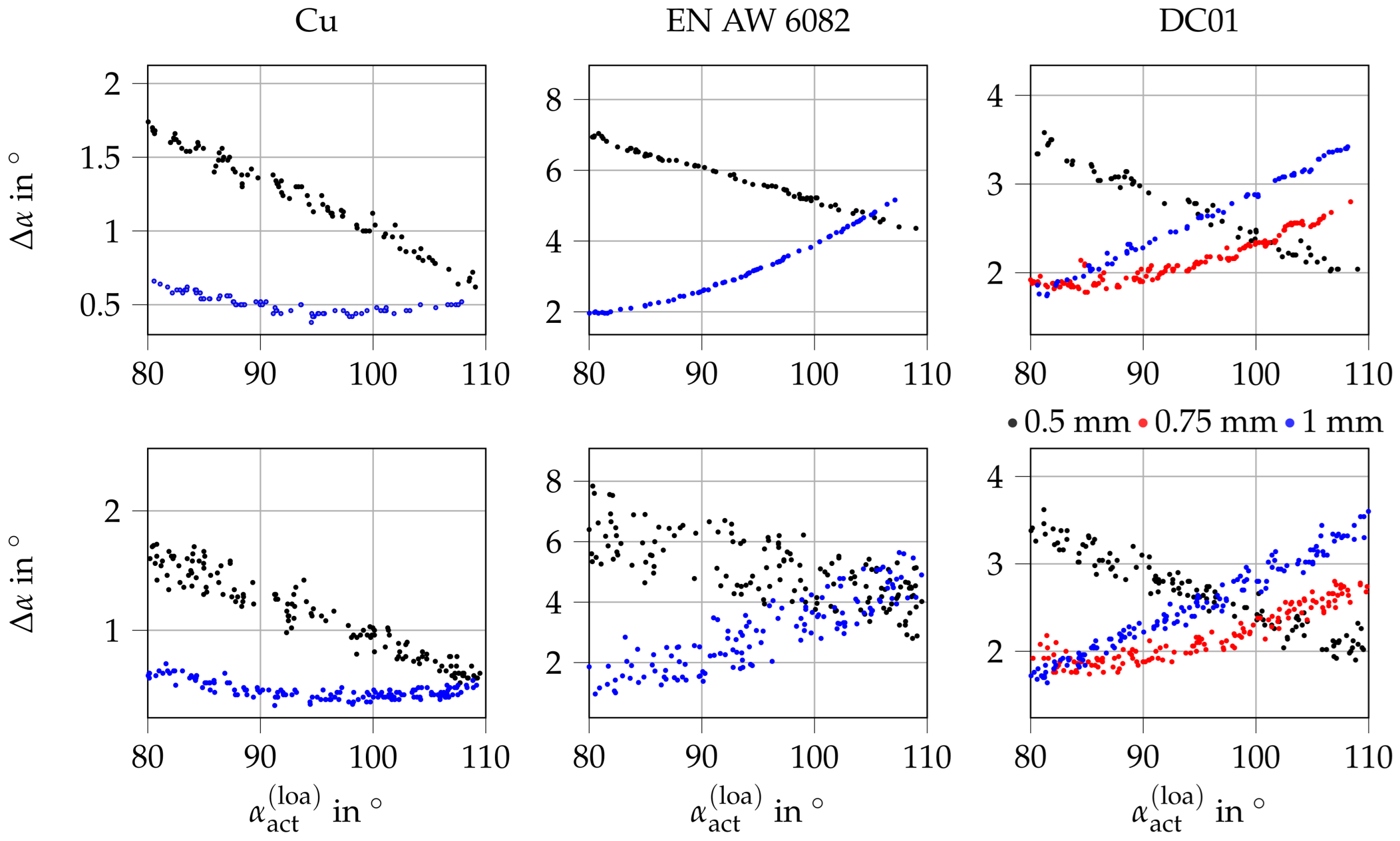
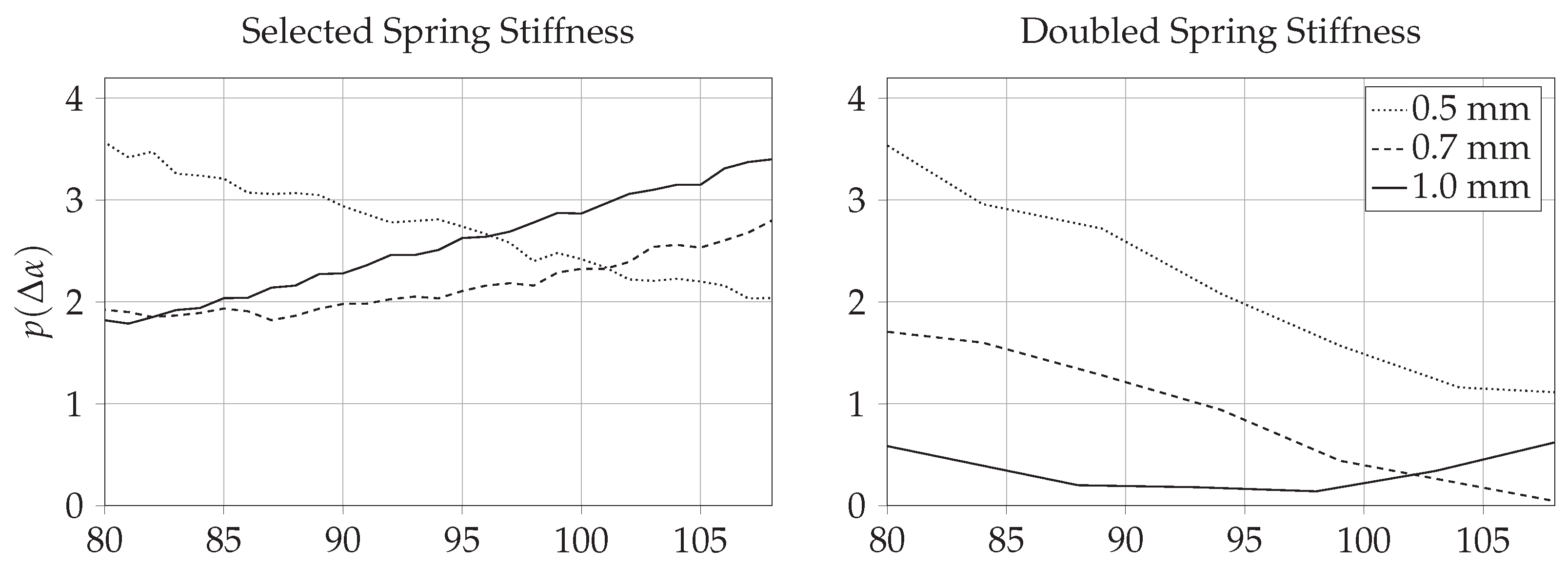
4.1. Simulative Results
4.2. Experimental Results
5. Conclusions
Author Contributions
Funding
Institutional Review Board Statement
Informed Consent Statement
Data Availability Statement
Conflicts of Interest
Abbreviations
| AC | Actor-Critic |
| DOAJ | Directory of Open Access Journals |
| DOF | Degrees Of Freedom |
| FEM | Finite-Element Method |
| LD | Linear Dichroism |
| MDPI | Multidisciplinary Digital Publishing Institute |
| Probability Density Function | |
| RL | Reinforcement Learning |
| SAC | Soft Actor-Critic |
| TLA | Three Letter Acronym |
References
- Möhring, H.; Wiederkehr, P.; Erkorkmaz, K.; Kakinuma, Y. Self-optimizing machining systems. CIRP Ann. 2020, 69, 740–763. [Google Scholar] [CrossRef]
- Allwood, J.; Duncan, S.; Cao, J.; Groche, P.; Hirt, G.; Kinsey, B.; Kuboki, T.; Liewald, M.; Sterzing, A.; Tekkaya, A. Closed-loop control of product properties in metal forming. CIRP Ann. 2016, 65, 573–596. [Google Scholar] [CrossRef]
- Volk, W.; Groche, P.; Brosius, A.; Ghiotti, A.; Kinsey, B.; Liewald, M.; Madej, L.; Min, J.; Yanagimoto, J. Models and modelling for process limits in metal forming. CIRP Ann. 2019, 68, 775–798. [Google Scholar] [CrossRef]
- Dornheim, J.; Link, N.; Gumbsch, P. Model-free adaptive optimal control of episodic fixed-horizon manufacturing processes using reinforcement learning. Int. J. Control Autom. Syst. 2020, 18, 1593–1604. [Google Scholar] [CrossRef]
- Idzik, C.; Krämer, A.; Hirt, G.; Lohmar, J. Coupling of an analytical rolling model and reinforcement learning to design pass schedules: Towards properties controlled hot rolling. J. Intell. Manuf. 2023, 35, 1469–1490. [Google Scholar] [CrossRef]
- Reinisch, N.; Rudolph, F.; Günther, S.; Bailly, D.; Hirt, G. Successful pass schedule design in open-die forging using double deep Q-learning. Processes 2021, 9, 1084. [Google Scholar] [CrossRef]
- Deng, J.; Sierla, S.; Sun, J.; Vyatkin, V. Reinforcement learning for industrial process control: A case study in flatness control in steel industry. Comput. Ind. 2022, 143, 103748. [Google Scholar] [CrossRef]
- Zhao, W.; Queralta, J.; Qingqing, L.; Westerlund, T. Towards Closing the Sim-to-Real Gap in Collaborative Multi-Robot Deep Reinforcement Learning. In Proceedings of the 2020 5th International Conference on Robotics and Automation Engineering (ICRAE), Singapore, 20–22 November 2020; pp. 7–12. [Google Scholar]
- Dulac-Arnold, G.; Levine, N.; Mankowitz, D.; Li, J.; Paduraru, C.; Gowal, S.; Hester, T. An empirical investigation of the challenges of real-world reinforcement learning. arXiv 2020, arXiv:2003.11881. [Google Scholar]
- Zünkler, B. Untersuchung des überelastischen Blechbiegens, von einem Einfachen Ansatz Ausgehend; Hanser Verlag: München, Germany, 1965; Volume 6. [Google Scholar]
- Gan, W.; Wagoner, R. Die design method for sheet springback. Int. J. Mech. Sci. 2004, 46, 1097–1113. [Google Scholar] [CrossRef]
- Zhang, Z.; Wu, J.; Zhang, S.; Wang, M.; Guo, R.; Guo, S. A new iterative method for springback control based on theory analysis and displacement adjustment. Int. J. Mech. Sci. 2016, 105, 330–339. [Google Scholar] [CrossRef]
- Wang, J.; Verma, S.; Alexander, R.; Gau, J. Springback control of sheet metal air bending process. J. Manuf. Process. 2008, 10, 21–27. [Google Scholar] [CrossRef]
- Heller, B.; Chatti, S.; Ridane, N.; Kleiner, M. Online-Process Control of Air Bending for Thin and Thick Sheet Metal. J. Mech. Behav. Mater. 2004, 15, 455–462. [Google Scholar] [CrossRef]
- Havinga, J.; van den Boogaard, T.; Dallinger, F.; Hora, P. Feedforward control of sheet bending based on force measurements. J. Manuf. Process. 2018, 31, 260–272. [Google Scholar] [CrossRef]
- Sharad, G.; Nandedkar, V. Springback in Sheet Metal U Bending-Fea and Neural Network Approach. Procedia Mater. Sci. 2014, 6, 835–839. [Google Scholar] [CrossRef]
- Liu, S.; Shi, Z.; Lin, J.; Yu, H. A generalisable tool path planning strategy for free-form sheet metal stamping through deep reinforcement and supervised learning. J. Intell. Manuf. 2025, 36, 2601–2627. [Google Scholar] [CrossRef]
- Fu, Z.; Mo, J. Springback prediction of high-strength sheet metal under air bending forming and tool design based on GA–BPNN. Int. J. Adv. Manuf. Technol. 2011, 53, 473–483. [Google Scholar] [CrossRef]
- Viswanathan, V.; Kinsey, B.; Cao, J. Experimental Implementation of Neural Network Springback Control for Sheet Metal Forming. J. Eng. Mater. Technol. 2003, 125, 141–147. [Google Scholar] [CrossRef]
- Molitor, D.; Arne, V.; Kubik, C.; Noemark, G.; Groche, P. Inline closed-loop control of bending angles with machine learning supported springback compensation. Int. J. Mater. Form. 2024, 17, 8. [Google Scholar] [CrossRef]
- Konda, V.; Tsitsiklis, J. Actor-Critic Algorithms. Adv. Neural Inf. Process. Syst. 1999, 12, 1–7. [Google Scholar]
- Haarnoja, T.; Zhou, A.; Abbeel, P.; Levine, S. Soft Actor-Critic: Off-Policy Maximum Entropy Deep Reinforcement Learning with a Stochastic Actor. arXiv 2018, arXiv:1801.01290. [Google Scholar]
- Shahzamanian, M.; Lloyd, D.; Partovi, A.; Wu, P. Study of influence of width to thickness ratio in sheet metals on bendability under ambient and superimposed hydrostatic pressure. Appl. Mech. 2021, 2, 542–558. [Google Scholar] [CrossRef]
- Doege, E.; Behrens, B.-A. Handbuch Umformtechnik: Grundlagen, Technologien, Maschinen; Springer: Berlin/Heidelberg, Germany, 2016; pp. 1–948. [Google Scholar]
- Groche, P.; Scheitza, M.; Kraft, M.; Schmitt, S. Increased total flexibility by 3D Servo Presses. CIRP Ann. 2010, 59, 267–270. [Google Scholar] [CrossRef]
- Molitor, D.; Arne, V.; Spies, D.; Hoppe, F.; Groche, P. Task space control of ram poses of multipoint Servo Presses. J. Process Control 2023, 129, 103057. [Google Scholar] [CrossRef]
- Unterberg, M.; Niemietz, P.; Trauth, D.; Wehrle, K.; Bergs, T. In-situ material classification in sheet-metal blanking using deep convolutional neural networks. Prod. Eng. Res. Dev. 2019, 13, 743–749. [Google Scholar] [CrossRef]
- Mulidrán, P.; Spišák, E.; Tomáš, M.; Rohal, V.; Stachowicz, F. The Springback Prediction of Deep-Drawing Quality Steel used in V-Bending Process. Acta Mech. Slovaca 2020, 23, 14–18. [Google Scholar] [CrossRef]
- Tseng, M.M.; Wang, Y.; Jiao, R.J. Mass Customization. In CIRP Encyclopedia of Production Engineering; Laperrière, L., Reinhart, G., Eds.; Springer: Berlin/Heidelberg, Germany, 2017. [Google Scholar] [CrossRef]
- Yang, D.; Bambach, M.; Cao, J.; Duflou, J.; Groche, P.; Kuboki, T.; Sterzing, A.; Tekkaya, A.; Lee, C. Flexibility in metal forming. CIRP Ann. 2018, 67, 743–765. [Google Scholar] [CrossRef]
- Schenek, A.; Görz, M.; Liewald, M.; Riedmüller, K.R. Data-Driven Derivation of Sheet Metal Properties Gained from Punching Forces Using an Artificial Neural Network. Key Eng. Mater. 2022, 926, 2174–2182. [Google Scholar] [CrossRef]


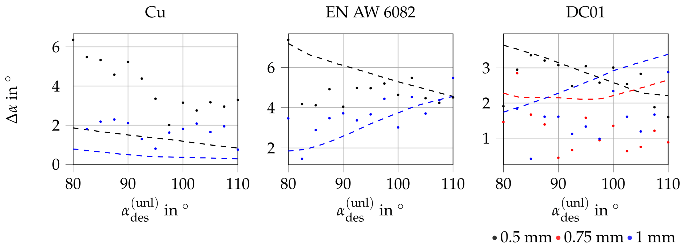
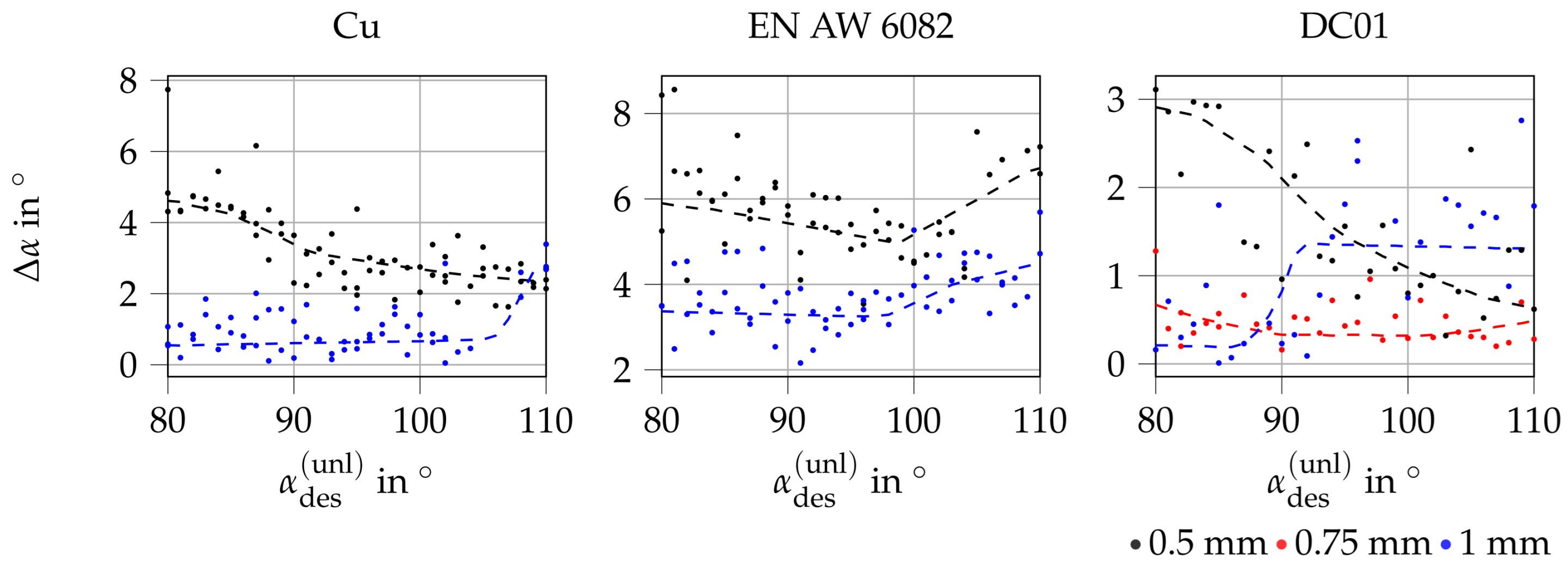
| Sheet Thickness [mm] | 0.5 | 0.75 | 1 |
|---|---|---|---|
| DC01 | x | x | x |
| EN AW 6082T6 | x | - | x |
| Copper | x | - | x |
| Learning Rate | Batchsize | |||
|---|---|---|---|---|
| Selected Hyperparameters | 128 | 0.05 | 0.1 | |
| Search Space | – | 8–256 | 0.01–0.2 | 0.01–0.2 |
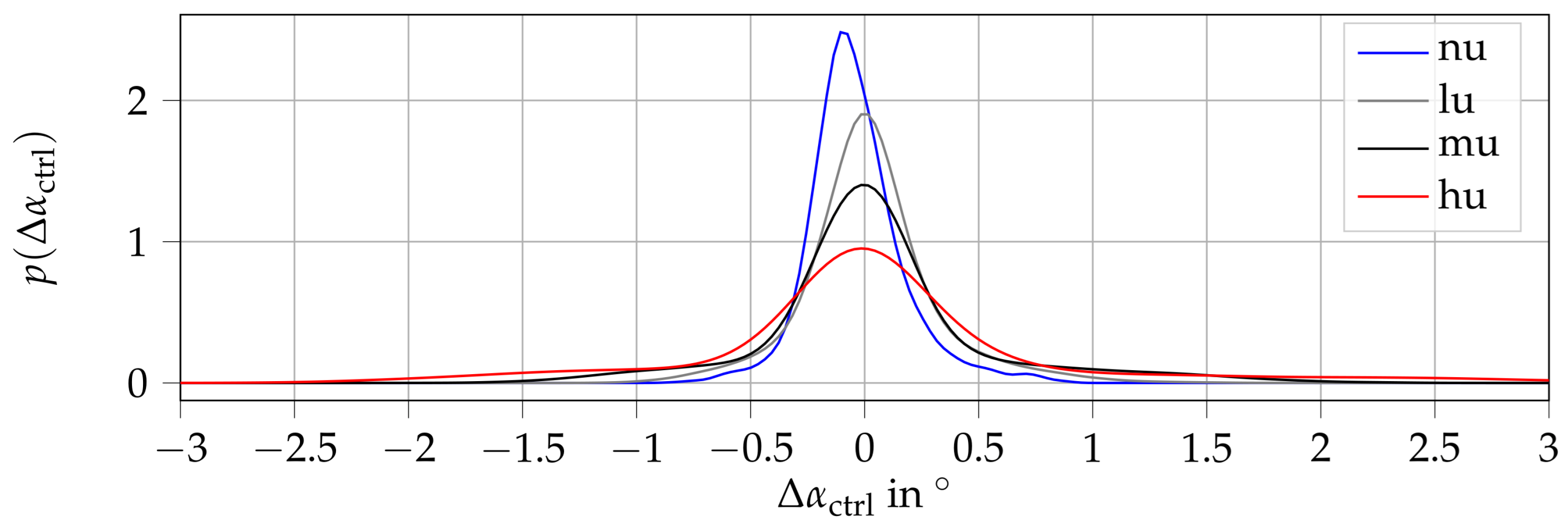
| Uncertainty | nu | lu | mu | hu |
|---|---|---|---|---|
| ±10,000 | ||||
| N | 3094 | 1725 | 3310 | 2069 |
| Metric | nu | lu | mu | hu |
|---|---|---|---|---|
| ° | ||||
| ° | - | |||
| ° | ||||
| ° | - |
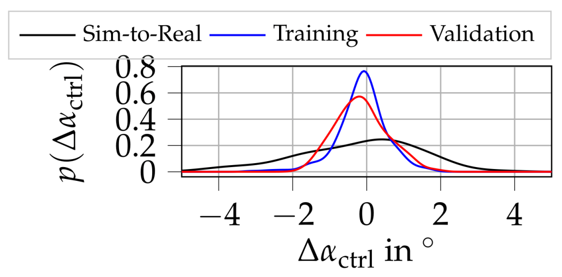
| Dataset | N | Stepsize | ° |
|---|---|---|---|
| Sim-to-Real | 95 | 2.5° | |
| Training | 330 | 1° | |
| Validation | 175 | 2.5° |
| Data Set | |||
|---|---|---|---|
| Sim-to-Real | 1.28 | 4.5 | −0.03 |
| Training | 0.48 | 3.13 | 0.88 |
| Validation | 0.57 | 1.86 | 0.86 |
Disclaimer/Publisher’s Note: The statements, opinions and data contained in all publications are solely those of the individual author(s) and contributor(s) and not of MDPI and/or the editor(s). MDPI and/or the editor(s) disclaim responsibility for any injury to people or property resulting from any ideas, methods, instructions or products referred to in the content. |
© 2025 by the authors. Licensee MDPI, Basel, Switzerland. This article is an open access article distributed under the terms and conditions of the Creative Commons Attribution (CC BY) license (https://creativecommons.org/licenses/by/4.0/).
Share and Cite
Veitenheimer, C.-V.; Molitor, D.A.; Arne, V.; Groche, P. Controlling Product Properties in Forming Processes Using Reinforcement Learning—An Application to V-Die Bending. Appl. Sci. 2025, 15, 5483. https://doi.org/10.3390/app15105483
Veitenheimer C-V, Molitor DA, Arne V, Groche P. Controlling Product Properties in Forming Processes Using Reinforcement Learning—An Application to V-Die Bending. Applied Sciences. 2025; 15(10):5483. https://doi.org/10.3390/app15105483
Chicago/Turabian StyleVeitenheimer, Ciarán-Victor, Dirk Alexander Molitor, Viktor Arne, and Peter Groche. 2025. "Controlling Product Properties in Forming Processes Using Reinforcement Learning—An Application to V-Die Bending" Applied Sciences 15, no. 10: 5483. https://doi.org/10.3390/app15105483
APA StyleVeitenheimer, C.-V., Molitor, D. A., Arne, V., & Groche, P. (2025). Controlling Product Properties in Forming Processes Using Reinforcement Learning—An Application to V-Die Bending. Applied Sciences, 15(10), 5483. https://doi.org/10.3390/app15105483