Abstract
In order to enhance the precision of network traffic prediction for multi-area vehicle networks, this paper proposes a two-tier distributed Software-Defined Vehicular Network (SDVN) architecture equipped with multiple controllers, which is subsequently deployed to manage traffic across regions, thus minimizing communication costs and enabling seamless vehicle movement. We firstly build on control plane placement (CPP) research, focusing on deployment strategies that impact scalability, performance, and fault tolerance. It highlights the importance of hierarchical decision-making with multiple controllers handling varying traffic demands. A comprehensive comparison of various machine learning and deep learning algorithms is then conducted to evaluate their efficacy in forecasting SDVN traffic patterns, which is crucial for system efficiency. Experiments show the proposed architecture’s effectiveness in traffic prediction and management in Shenzhen’s Longhua New District. The study confirms that the SDVN system enhances traffic prediction and management, improving urban mobility and Internet of Vehicles. The paper offers a framework using advanced technologies to address challenges in traffic prediction and management in modern vehicular networks.
1. Introduction
In the Internet of Vehicles (IOV) environment for intelligent transportation systems (ITSs), the usage rate of audio, video, text messages, and other content has increased, which limits the available bandwidth and resources of other applications. In recent years, as cloud computing and edge computing have become important means to assist ITSs in information transmission [1], ITS applications and use cases have become more diversified and specialized. On-Board Unit (OBU) cloud [2,3,4], Road-Side Unit (RSU) cloud [5] and hybrid cloud [6] provide a basic environment for communication protocols, computing infrastructure, services, and applications to improve the efficiency of the IOV. Data center networks and wide area networks are increasingly adopting the Software-Defined Network (SDN) paradigm, which also brings the emergence to use SDN for managing the IOV network. The cloud resource manager is responsible for calculating the network configuration for the change in network requirements from time to time to meet the dynamic characteristics of the network.
As shown in Figure 1 below, the vehicle can communicate with the RSU cloud. The communication in the cloud is managed by the OpenFlow controller, and its basic computing unit is the virtual machine on the Road-Side Unit server. Considering the QoS requirements, it is necessary to combine computer and link load balancing for cloud resource management. By deploying MEC servers near the available base stations connecting vehicles, SDN cloud resource management provides higher-performance operations for data centers and edge servers. It helps edge computing operate in near-optimal conditions. While obtaining continuous services from edge servers, due to mobility and cloud resource management requirements, virtual machines (VMs) need to switch from one Cloudlet to another Cloudlet. In order to achieve smooth operation in a dynamic environment, SDN needs to be used to reshape the network infrastructure to achieve efficient cloud resource management. As for the SDN, the Controller Placement Problem (CPP) of SDN multi-controller needs to be considered in the cooperative communication of medium- and large-scale SDNs [7,8]. CPP is an important part of SDN design, and the controller layout depends on the goal of network design. Without loss of generality, for the placement of SDN controllers, the existing literature has the most research on two representative targets: network delay and number of controllers. Heller et al. [9] first proposed to study the multi-controller placement problem in SDNs. They considered the number of controllers, the location of controllers, and the switches assigned to each controller in CPP. Wang et al. [10] used a k-means-based network partitioning algorithm to solve the CPP problem, which aims to minimize the delay of the switch controller. Zhao et al. [11] Addressed the challenge of controller deployment in software-defined networking via affinity propagation, where an improved clustering approach inspired by exemplar-based techniques and leveraging affinity propagation is introduced. In the study on switch–controller interactions, Zhang et al. [12] highlighted the critical role of inter-controller communication, developing a latency analysis model based on two distinct inter-controller data ownership frameworks. Zeng et al. [13] studied CPP to ensure the flow establishment time. It is assumed that the control load on each switch obeys Poisson distribution, and the service time on each controller obeys exponential distribution.
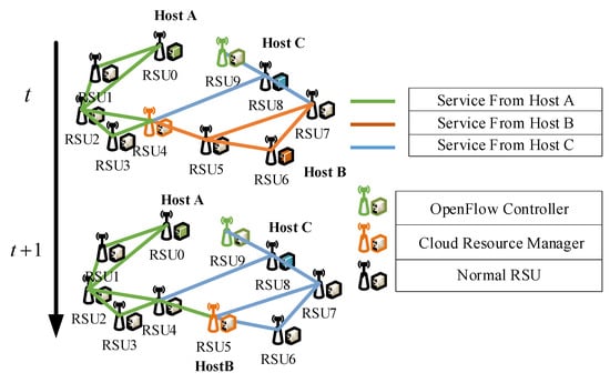
Figure 1.
Energy consumption node relationship network diagram.
1.1. Related Works
Han et al. [14] studied CPP in SDNs based on classical control theory. They defined the control delay as the number of time slots required to drive the network from one state to another, and proposed two complementary heuristic algorithms: a controller-minimization approach optimizing propagation latency under resource constraints, and a delay-constrained optimization strategy achieving minimal controller deployment while satisfying predefined latency thresholds.
Another aspect of CPP has aroused great interest in the industry, that is, the use of graph theory, game theory, queuing theory, and other concepts to model CPP. In general, the location problem exists in many scientific problems, such as virtual machine placement [15] and sensor placement in wireless sensor networks [16]. These exemplify problem configurations that share conceptual similarities with the Controller Placement Problem (CPP) in software-defined networking architectures, because their core is the classic facility location problem [17].
In all, CPP problems based on different optimization objectives cover a wide range of scientific problems. In the existing research, in order to obtain a suitable CPP solution, various methods are studied, including optimal strategy, heuristic strategy, and classical control theory. With the popularity of SDN in an array of sectors, such as data centers, wide-area networks, and mobile networks, CPP has been developed in emerging applications. Several aspects of CPP are worth noting, which can be considered from the perspective of different goals such as network responsiveness, fault tolerance, and load balancing. In previous CPP research, the optimization of a single target was the most important; for the multi-objective CPP problem, it is usually necessary to consider the weight between multiple conflicting targets. For example, in order to optimize the switch controller delay, the controller needs to be evenly distributed over the network, but this will increase the number of controllers in the network.
The Internet of Vehicles is essentially a (VANET) composed of vehicle OBUs and fixed road infrastructure such as RSUs and base stations. In the existing research of vehicle networking, He et al. [18] introduced a converged architecture for vehicle-to-everything (V2X) networks that synergistically integrates edge caching and distributed computing paradigms, employing deep reinforcement learning frameworks to co-optimize multidimensional parameter spaces within the system model. For a multi-area vehicle network with multiple controllers, each controller is responsible for processing most of the information in its area. Therefore, this section first proposes a delay-optimized SDVN system architecture model, which is composed of a two-layer distributed control plane architecture and refers to the HyperFlow distributed controller architecture [19] to reduce the delay caused by system/operation, as shown in Figure 2:
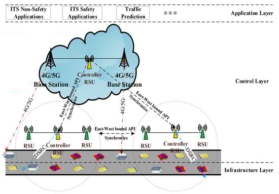
Figure 2.
Software-Defined Vehicular Network paradigm.
As shown in Figure 2, in SDVN, different RSUs are connected through a broadband link, and the controllers synchronize the network state through an east–west interface. The controller is selected from a number of RSUs interconnected by wired links. The controller RSU is actually a combination of ordinary RSUs and SDN controllers. In addition, different regions of SDVN often have different traffic characteristics, and some global information flows may need to be forwarded between multiple regions. As traffic occurs in different areas that may belong to different service providers, it is necessary to use multiple controllers, at least one of which controls a single area. The controller of each region is responsible for its own region, but inter-domain communication should be performed to provide reliable data transmission [20]. The data plane consists of On-Board Units (OBUs) and conventional Road-Side Units (RSUs), with each OBU equipped with both a DSRC interface and a 4G/5G interface. The 4G/5G interface is exclusively activated when the OBU is outside the coverage of RSUs. This design ensures that compared to traditional SDVN systems, communication costs are significantly reduced by leveraging cellular connectivity only when necessary. In general, the OBU can obtain information about the nearby controller through the Basic Safety Message (BSM) broadcast by the RSU. When the vehicle is within the coverage of the RSU, the OBU is connected to the RSU controller through the V2I and V2V links, and the same link will also be used for data communication, which is called in-band control. When the vehicle moves between RSUs under different controllers, a simple switching mechanism based on signal strength is adopted. When a vehicle exits the coverage of an RSU (Road-Side Unit), the OBU (On-Board Unit) aboard leverages a dedicated 4G/5G communication channel to establish a connection with the base station. Since this channel is exclusively allocated for control and data plane communication, this specific mechanism is termed out-of-band communication. SDVN requires additional periodic collection of network information, which serves as the foundation for the control plane to enable precise and intelligent decision-making. Most existing SDVN (Software-Defined Vehicular Network) systems leverage cellular links to acquire such network information, which will generate additional communication overhead and cost. In the proposed SDVN, the communication overhead and cost pressure can be shared by the DSRC communication mode in the RSU. In SDVN, the RSU listens to regular BSM broadcasts to collect network information such as vehicle location and speed. Based on the retrieved information, the estimated distance of the vehicle, and the knowledge of the local road network, a local topology is generated. Initially, the topology information is transmitted to the nearest local controller. Subsequently, all controllers synchronize and integrate all the information received from the Road-Side Unit (RSU) to create an aggregated area network diagram.
For On-Board Units (OBUs) outside the RSU coverage area, they are required to adhere to the existing state update mechanism. They send beacon messages to the nearest controller via the 4G/5G interface. In this scenario, the frequency of network information exchange is set to be consistent with the Basic Safety Message (BSM) frequency, because the network topology changes only when a new BSM arrives.
In SDVN, Vissicchio et al. [21] investigated hybrid SDN architectures that integrate SDN with traditional distributed network models, presenting use cases that demonstrate how these hybrid approaches address the shortcomings of both models and provide compelling reasons for a partial shift to SDN. When the sender wants to send information to the receiver, the process is as follows: (1) When the packet arrives as the first packet of the data stream from the sender to the SDVN switch, for this packet, the SDVN switch checks the flow rules by matching it with the flow table entries in the SDVN cache. (2) If a matching entry is detected in the flow table of the SDVN switch, the instruction associated with a specific flow entry is executed, such as ‘packet/matching field’, ‘update counter’, etc. After that, the data packet is directed to the relevant receiver. If there is no matching item in the flow table of the switch, the data packet is directed to the controller through the secure channel. (3) In the data transmission phase, when the OBU receives a packet from an unknown destination port, the OBU sends a PACKET-IN message to the nearest controller. After that, the RSU controller analyzes the source IP address and the target IP address in the packet according to the request type and the availability of the information, and updates the switch flow table entries in the southbound API, the OpenFlow protocol path, to calculate the path required from the source node to the destination node. All (1), (2), and (3) working processes are shown above in Figure 2.
1.2. Influencing Factors of SDN Controller Deployment
The SDN control plane includes one or more controllers, and the SDNs with multiple controllers can communicate with each other through the east–west protocol. For small-scale regional networks, a single controller is sufficient [9]. However, the scalability and information transmission efficiency of large-scale multi-area networks increase the demand for multiple controllers in SDN [22,23]. The main differences between a single controller and multiple controllers are shown in Figure 3:
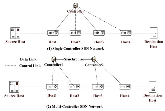
Figure 3.
SDN comparison of single controller and multiple controllers.
As shown in Figure 3(1), the controller is responsible for controlling four routers when there is a single controller, while there are two controllers in Figure 3(2). In this case, the network state replicates and synchronizes between the two controllers. For the control plane deployment with multiple controllers, the following problems will arise: How can we better perform state synchronization? How many controllers should be placed in the SDN, and how should the controllers be deployed? When there are multiple controllers, it is essential to consider how to make it more efficient to determine the placement of the SDN control plane. The above problems further promote the research of SDN control plane placement problem, namely CPP. For the influencing factors of CPP, the following four aspects are analyzed:
- (1)
- Controller location. In the SDN, the expected position of the controller is regarded as a subset of the set of switch positions. This design choice makes SDN migration easy, because traditional switches are gradually replaced by SDN switches and configured SDN controllers, thereby eliminating changes to the existing network layout.
- (2)
- Number of control devices. The key to studying CPP is to find the number of controllers, but the number of controllers is usually regarded as an input. In most of the existing research literature, the number of controllers is obtained by analysis ([24,25]) or experience ([13,26]).
- (3)
- Control command load. The load modeling generated by SDN switch control commands is different for single-area and multi-area networks. For single-area networks, the load from the SDN switch includes the load control packets it generates. However, for multi-area networks, the SDN switch control load is regarded as the sum of the load packets generated by it and the load from adjacent switches belonging to different regions [27]. In the SDVN, it is necessary to analyze and predict the network traffic, and then perform load balancing.
- (4)
- Controller processing delay. Compared with the propagation delay of switches, most studies ignore the processing time of SDN controllers. However, the control delay experienced by SDN switches is a key design consideration for the placement of SDN controllers, which directly affects the information transmission efficiency of SDVNs. In large-scale SDVNs, delay is positively correlated with distance, that is, the farther the distance, the greater the delay.
The organizational structure of this article is as follows. Section 2 focuses on the methodology, that is communication delay parameters between vehicles and RSUs, mathematical model construction of control plane deployment, and the deterministic annealing clustering algorithm. Section 3 explores the SDVN traffic analysis and prediction in detail, and has presented the results of the experiment. Finally, in Section 4, a conclusion is drawn.
2. Methodology
The RSU uses the existing DSRC wireless link as the southbound interface, and the research on the communication contact characteristics between vehicles and intersections [28] also promotes the use of the RSU as the physical carrier of the SDN controller. However, a single controller in the RSU often fails to cover the entire vehicle network; that is, a single controller will not be able to hold enough network view or control area. Therefore, for the entire multi-area vehicle network SDVN, a set of RSU placement controllers need to be selected, and the controllers can communicate with each other, so that they have sufficient control areas in the vehicle network.
2.1. Communication Delay Parameters Between Vehicles and RSUs
In addition, it should be ensured that the time for the vehicle OBU to reach the control plane is within a given threshold range. For the SDN architecture, a northbound interface is also required to connect the application deployment. Since the application deployment is completed in the IP network, to establish a secure channel between controllers, they must be situated on the same IP network. For Software-Defined Vehicular Networks (SDVNs), several crucial factors need to be taken into account. These include the physical positioning of the controllers, the interaction between the control plane and the data plane, and the functional demarcation within the system. This ensures that the SDVN can operate efficiently and securely, leveraging the proper placement and interaction of its components to manage network traffic and services effectively. The controller needs to process requests for network information in specific areas, such as vehicle statistics, road conditions, and network traffic statistics. The communication requests on the road are either redirected by the controller or received directly from the OBU that is not covered by the RSU. After processing the incoming requests, the controller will pass them to the OBU by controlling the ordinary RSU or directly passing them through 4G/5G, depending on the type of request (such as real-time, non-real-time) and the reachability of the OBU (whether they are within the RSU coverage or not).
The delay generated in the SDVN is mainly determined by the location and communication mode of the SDVN controller relative to the SDVN node. Deng et al. [29] carried out a comprehensive comparison and in-depth analysis of the majority of the existing centralized Software-Defined Vehicular Network (SDVN) architectures. These architectures offer the advantage of endowing Vehicular Ad Hoc Networks (VANETs) with flexibility and programmability. However, this benefit is achieved by sacrificing latency. Therefore, in order to make SDVN more promising, it is necessary to consider the quality of service requirements of VANETs applications (such as the delay requirement of intelligent transportation system security applications being less than 100 ms); delay should be given a higher-priority consideration. As a solution to some of the above key issues, in order to reduce the communication delay, the control layer can be reduced to the vehicle and RSU end.
This part discusses in detail the background knowledge related to the controller configuration problem, including the factors that affect the controller configuration, and the theoretical analysis of the time-delay parameters required to describe the problem.
A simple method is to place a controller on each RSU so that the OBU can communicate directly with the SDN controller. Since the controller RSU needs to have both DSRC and LTE interfaces, the general cost is high and complicated. Obviously, placing the controller on all RSUs will increase the cost and complexity of the entire system. On the other hand, a single RSU may not have the minimum network topology state required for accurate routing decisions. At the same time, moving vehicles will only stay in an RSU coverage for a short period of time, which will lead to frequent switching between SDN controllers, which is not desirable. According to the research of [28], the communication contact characteristics between vehicles and intersections in SDVNs have been studied. The complementary cumulative distribution function (CCDF) for the contact duration is presented as follows:
where and . From the above equation, the average contact time is given by Formula (2):
It can be deduced that the average contact time is 2.67 min. The resulting experimental contact time between the vehicle and the RSU in urban areas is a moderate value. In order to avoid frequent switching, it is always desirable to maintain a high contact duration with the SDN controller.
2.2. Mathematical Model Construction of Control Plane Deployment
In terms of the number of controllers, it is hoped that the number of controllers is small, and the number of ordinary RSUs connected to each controller is large. However, if fewer controllers are used, the vehicle OBU far away from the controller RSU may experience considerable delay. In order to ensure that a single RSU controller does not overload, the average distribution of workload between RSU controllers is also a key factor to be considered. The number of ordinary RSUs connected to the RSU controller can be used as a measure of its workload. Because of the higher number of ordinary RSUs, the larger coverage area means a greater number of connected vehicles, and a greater workload. The above situation is particularly important in high-density urban road networks.
Based on the above analysis, considering the network load, the number of RSUs, the location of RSUs, and the delay, the controller deployment model is given as follows: the definition represents the set of all RSU nodes, and and represent the set of candidate RSU nodes that can be used as RSU controllers, . Among them, all controllers in the SDVN can communicate directly with each other; denotes the number of RSUs that a single RSU controller can control, . One or more of these RSU nodes can be specified as controllers, and the optimal number and location of these controllers depend on a variety of factors, such as delay, distance, etc. All controllers can be connected to each other not only with ordinary nodes, but also with controllers. Therefore, there will be a synchronization cost between ‘controller pairs’.
In addition, represents the location of the node in the wireless network; represents the controller deployment strategy. If the node is selected to play the role of controller, then the converse is true. Similarly, we determine the controller allocation strategy, where if the node is allocated to the controller , then , otherwise . denotes the communication delay between nodes and , assuming that the delay is proportional to the square of the Euclidean distance, i.e., [30]. According to the above analysis, the objective function of the optimal allocation of the controller is expressed as Equation (3), and the constraint conditions are shown as Equations (4)–(7):
Subject to
In Equation (3), the first term of the objective function pertains to the communication delay between all nodes and the controller, while the second term denotes the synchronization delay among all controllers. Moreover, the synchronization delay is also contingent upon the number of nodes assigned to the controller. The constraint (4) indicates that each node is assigned to only one controller. Constraint (5) ensures that the node assignment of the controller is only performed on the specified controller node. The parameter represents the relative weight of the communication delay between the controller and the node relative to the synchronization delay between the controllers. Constraint (6) and constraint (7) represent variables, which are binary variables, and their values range from 0 to 1. The above problem is a multi-objective, mixed-integer, non-linear problem (MMINLP), and its complexity is NP-hard. Existing algorithms cannot guarantee finding the global optimal solution, but can approach the optimal solution. Considering the characteristics of various heuristic algorithms, the deterministic annealing clustering (DAC) algorithm is used to solve the above problems.
2.3. Algorithms of Deterministic Annealing Clustering
Under the setting of the deterministic annealing clustering algorithm, the expected distortion is defined as follows:
where is the geospatial coordinate of each RSU node, is the cluster center point that needs to be calculated, that is, the position coordinates of the RSU controller. is the probability of correlation between the point , the cluster center , is the deviation measure, and the square Euclidean distance is usually selected. will be defined as giving the relative importance of the first node, assuming , if there is no other explanation. System entropy can be defined as . In addition, the free energy of the system is defined, where is the temperature of the system. Note that can be regarded as a Lagrangian function with the main goal of minimizing , where is a Lagrangian multiplier. The cluster center iteration of the DAC algorithm can be summarized as sequentially optimizing the self-parameters corresponding to , namely the correlation probability and the cluster center position.
Firstly, the distortion is defined. Specifically, the distortion between an edge Road-Side Unit (RSU) node and a controller is determined not solely by the communication delay between these two nodes. It also hinges on the distance from other controllers. This means that the distortion between the edge RSU node and the controller depends not only on the communication delay between the two nodes, but also on the distance from other controllers . In order to observe the relationship between (3) and (7), the total distortion of the model can be summarized as follows:
We replace the hard assignment with the soft correlation probability . As mentioned above, we define the free energy of the system , and let the partial derivative of the free energy term with respect to the correlation probability be zero:
Therefore, the correlation probability obeys the Boltzmann distribution. Similarly, let the derivative with respect to the cluster center be zero, and the following linear equations can be obtained:
where , and can be calculated by Bayesian rule . This gives us a linear system of variables , where and are the number of cluster centers and the dimension of the data, respectively. For the convergence of the deterministic annealing clustering algorithm, it is essential that the linear equations always have solutions.
Theorem 1.
Given a linear system of Equation (11) as defined above, if , then there is always a unique solution , where the coefficient matrix associated with the system of equations is non-degenerate, its determinant is ; the detailed DAC algorithm pseudo-code is as follows:
As shown in Algorithm 1, a large number of experiments are first needed to determine the tolerance level . For the convergence test, if , then for a predetermined level of tolerance , stop the iteration . In the last line of the DAC algorithm, it specifies the node closest to each cluster center as the controller. The iterative complexity of the algorithm depends on the following four points: (1) Calculate , for , the square of the Euclidean distance; (2) Perform a similarity calculation of the distance between cluster centers; (3) Calculate the correlation probability; (4) Solve the linear equations. The complexity of the above four operations is , , , and , respectively. When is large, is dominant. Therefore, for the maximum number of iterations , the computational complexity of the algorithm is , which is linear with the data size, the maximum number of cluster centers, and the data dimension.
| Algorithm 1: Deterministic Annealing Clustering Algorithm |
| Set the maximum number of cluster centers Kmax and minimum temperature Tmin; |
| Initial: ; |
| while convergence do |
| Update: |
| Solve: |
| Update: ; |
| if then |
| Break; |
| else: |
| Cooling steps: ; |
| Randomly generate small vectors ; |
| use ; |
| End |
| End |
| For , do the last step of iteration; |
| ; |
2.4. SDVN Controller Deployment Results
Mininet simulation software was developed for experiments, and a computational verification environment was established for deterministic annealing clustering algorithms and machine learning. Deep learning Keras was built on a desktop computer with the following hardware and software configurations: an AMD Ryzen 7 1800X Eight-Core Processor with a clock speed of 3.60 GHz as the CPU, a Ubuntu 20.04 operating system, 8 GB of RAM, and an NVIDIA GeForce GTX 1060 6 GB as the GPU, which is shown in Table 1.

Table 1.
Experiment configuration.
As show in Table 1, the experimental simulation case selects the streets of Longhua New District, Shenzhen, and builds a multi-area SDVN composed of 42 RSUs in the Mininet simulation environment. Each RSU is connected by a wired network, and most of them are deployed on the main road and the secondary road, as shown in Figure 4:
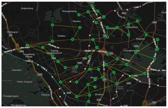
Figure 4.
Urban road environment SDVN topology.
Figure 4 depicts a large-scale SDVN consisting of 46 RSUs. The green dots in the graph represent RSUs. Each RSU is composed of OpenFlow switches and servers, labeled from 0 to 45. The ‘location’ results of the controller solved by the DAC algorithm are shown in Figure 5.
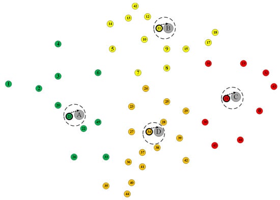
Figure 5.
Result of SDVN controller deployment.
As shown in Figure 5, the four controller RSUs obtained by solving are No. 21, No. 34, No. 11, and No. 31 RSUs, respectively. In Figure 5, the four controller RSUs and the surrounding ordinary RSU areas are distinguished by green, yellow, red, and orange, respectively. The four controller RSUs are highlighted and represented by four gray circles of A, B, C, and D, respectively.
Because it is impossible to collect traffic information for all vehicles in the road network, in order to predict SDVN traffic (mainly to predict the level of network traffic, which can provide a basis for network load balancing research), the traffic information provided by taxis (or ride-hailing) equipped with GPS equipment was used for analysis. Every GPS-equipped taxi (or ride-hailing car) periodically reports traffic information to the surrounding RSU. The sampling period is set as 1 s, that is 1 Hz in the application scenario. Since each RSU is located in different parts of the city, the real-time traffic flow and road conditions are different, which will result in a large difference in the information interaction requirements of different RSUs. Therefore, after obtaining the network traffic collected by taxis (or online car-hailing) in the region, the network traffic level of the SDVN after control plane deployment in the region in the future is predicted; SDVN traffic prediction can provide a basis for judging the network load balancing when all urban road vehicles are connected to the network in the future [31].
3. SDVN Traffic Analysis and Prediction
The collected traffic information is summarized and analyzed. Some data flow information is shown in Table 2:
Table 2.
Data flow.
As shown in Table 2, the table has eight fields, namely ‘number’, ‘number of packets’, ‘packet size’, ‘source address’, ‘target address’, ‘switch number’, ‘traffic size’, and ‘controller’. Taking the 0th datapoint as an example, the number of data packets in the data stream is 1, the size of the data packet is 42 Bytes, the source address is 10.1.1.2, the target address is 10.1.1.6, the switch number used is 1, the traffic size is ‘low’, and the connected controller RSU is A. The number of data streams flowing through the four controllers A, B, C, and D is 240, 166, 213, and 220, respectively; after statistical summary analysis, the flow size and proportion of different controllers are shown in Table 3, where 0 indicates ‘low’ and 1 indicates ‘high’.
Table 3.
The data flow and its proportion of different controller RSUs.
As shown in Table 3, the proportion of high and low flow through A controller is 50.00% and 50.00%, respectively. The proportion of high and low flow through B controller is 45.18% and 54.82%, respectively. The proportion of high and low flow through C controller is 38.03% and 61.97%, respectively. The proportion of high and low flow through the D controller is 31.82% and 68.18%, respectively. The number of ‘high’ and ‘low’ data streams flowing through each controller is shown in the fourth column. The traffic information provided by taxis equipped with GPS equipment (or online ride-hailing) is summarized, and the total number of data streams flowing through the four controller RSUs is 839.
The purpose of placing controllers is to minimize the number of controllers required to cover a given network map while placing them at RSUs with significant locations. On the other hand, it is also necessary to allocate workloads fairly between controllers. The data set is divided into a training set and a test set, with 639 training sets and 200 test sets. The process of creating a training set and a test set is as follows. Corresponding to the four controllers A, B, C, and D, 839 network traffic datapoints of the overall data set are randomly sampled. Each controller obtains 50 instances, making a total of 200 pieces of network traffic information; the remaining 639 pieces of network traffic information form the training set. The ratio of large and small traffic corresponding to the 50 pieces of network traffic information of the four controllers A, B, C and D in the test set after sampling is shown in Table 4:
Table 4.
The data flow ratio of different controller RSUs in the test set.
As shown in Table 4, for the flow size column, the value ‘0’ means ‘low’ and ‘1’ means ‘high’. The flow composition flowing through A controller is ‘high’:‘low’ = 50.00%:50.00%; the flow composition of B controller is ‘high’:‘low’ = 32.00%:68.00%; the flow composition of C controller is ‘high’:‘low’ = 38.00%:62.00%; and the flow composition of D controller is ‘high’:‘low’ = 44.00%:56.00%.
In order to predict the size of network traffic, the data set is divided into a training set and test set, of which the training set contains 639 data and the test set 200. At the same time, the training set is further divided: 511 data are used for training, and 128 data are used for verification. Since the traffic is classified by size, the subsequent traffic prediction problem is a binary classification problem. In solving this problem, the binary cross entropy is used as the loss function. The following formula of binary cross entropy is given:
is a binary label, with a value of 1 or 0, indicating the probability of belonging to the label.
Next, a sequential model neural network is built using the deep learning Keras framework. The optimizer of the sequential model neural network is adaptive moment estimation (Adam), the loss function is binary cross entropy, and the evaluation index is accuracy. Its detailed neural network structure is shown in Figure 6:
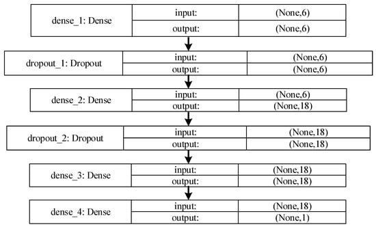
Figure 6.
Sequential neural network model structure.
As shown in Figure 6, the sequential model neural network is a linear stack of multiple network layers. The first layer of the sequential model requires the dimension of the input data. For the first layer, that is, the dense_1 layer, Dense represents the full connection, and ‘input’ represents the input of a tuple type of two-dimensional data (None, 6); if none is filled in, it means that the position value is any positive integer. The output ‘output’ of the first layer is also a two-dimensional data of tuple type (None, 6). For the second layer dropout_1, Dropout represents random deactivation, and in the forward propagation process of the model training stage, the activation value of some neurons stops working with a certain probability, so that the generalization of the neural network is stronger. The back layers refer to the first two layers, and so on. The following network layers can automatically derive the dimension of the intermediate data, and the ‘output’ of the last layer has a two-dimensional data dimension (None, 1). The data of 639 training sets were further divided into 80%—that is, 511 were used as new training sets—and 20%—that is, 128 were used as validation sets. After iteration, the loss function value and accuracy of the sequential model change with the number of iterations as shown in Figure 7, where blue represents the training set and red represents the validation set:
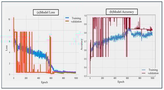
Figure 7.
The sequential model loss function value and accuracy rate change with the number of iterations.
Figure 7a,b represent the loss function value and accuracy of the sequential model neural network with the change in the number of iterations on the training set and the verification set, respectively. In the training process, the loss function value and accuracy of the validation set fluctuate greatly before 600 iterations. After 800 epoch iterations, the loss value and accuracy of the model on the training set and the verification set gradually converge. Finally, at the 1000th epoch iteration, the loss function value of the model on the training set is 0.4131, and the accuracy rate is 0.7769. At this time, the loss function value of the model on the verification set is 0.2803, and the accuracy rate is 0.8281.
In addition, after training the sequential model neural network in the training set and the verification set, the model is further applied on the test set with 200 network traffic. The loss function value is 0.3236 and the accuracy rate is 0.8550. Further, the four commonly used machine learning classifiers XGBoost classifier, Random Forest classifier, Logistic Regression, and Support Vector Machine (SVM) are used to classify the traffic level of the training set data. The training process is shown in Figure 8:
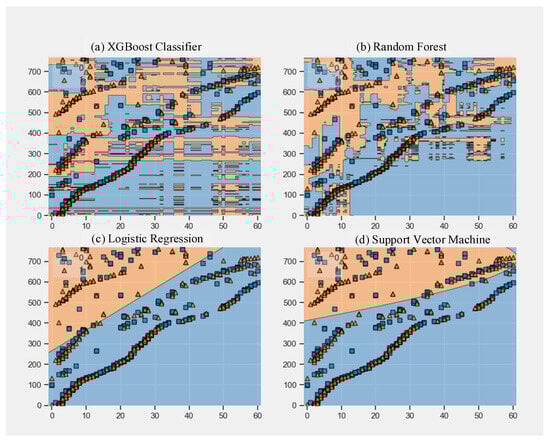
Figure 8.
Iterative process of four machine learning classifiers.
Figure 8a–d correspond to XGBoost classifier algorithm, random forest algorithm, logistic regression algorithm, and support vector machine, in turn. After a lot of parameter adjustment and experimental comparison, one of the best initial parameters is selected for each algorithm. Due to the characteristics of the machine learning algorithm, it is impossible to guarantee that the parameter is the best for each training. But it can be as close to the best as possible. The parameter settings of each machine learning algorithm are as follows. XGboost classifier algorithm parameter settings: the learning rate = 0.3, the minimum leaf node sample weight sum = 1, the maximum depth = 6, the maximum number of leaves on the tree = 6, and the remaining parameter settings are default. Random forest algorithm: the number of decision trees = 200, there is a back sampling, there is no limit on the maximum number of leaf nodes, and the remaining parameters are set to default. Logistic regression algorithm: Solver = quasi-Newton method, the maximum number of iterations = 500, and the remaining parameters are default. Support vector machine algorithm: classification error penalty coefficient = 1, random seed = 20, kernel function = Radial Basis Function (RBF), the rest of the parameters are set as default.
The accuracy and standard deviation of the above four machine learning algorithms and deep learning algorithms (sequential model neural network) are summarized and compared. And the integrated model is further designed, as shown in Figure 9:
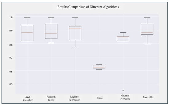
Figure 9.
Accuracy box plot for six algorithms.
As shown in Figure 9, the five algorithms from left to right correspond to XGBoost algorithm, random forest, logistic regression, support vector machine, and sequential model neural network. For the XGBoost algorithm, the average accuracy is 0.89, and the standard deviation is +/−0.07. The average accuracy of the random forest algorithm is 0.89, and the standard deviation is +/−0.07; the average accuracy of logistic regression is 0.89, and the standard deviation is +/−0.08. The average accuracy of the support vector machine algorithm is 0.63, and the standard deviation is +/−0.01; the accuracy of the sequential model neural network algorithm is 0.77, and the standard deviation is +/−0.16. Among them, the classification accuracy of the support vector machine (SVM) algorithm is the worst, and the average accuracy is 0.63. Therefore, combining the accuracy of the above four machine learning algorithms and the sequential model neural network algorithm, it was decided to remove the support vector machine algorithm and design an ensemble learning algorithm model (ensemble model). The ensemble algorithm integrates XGBoost classification algorithm, random forest, logistic regression, and sequential model neural network to implement an ensemble classifier using weighted majority voting technology to improve accuracy. The voting weight of XGBoost algorithm, random forest, logistic regression and sequential model neural network is set as 1:1:1:0.8. The rightmost of Figure 9 is the box plot of the integrated algorithm, with an average accuracy of 0.90 and a standard deviation of +/−0.07. According to the research of [32], they believe that the current traffic prediction method based on deep learning has better performance than the traditional prediction method. However, in this section, the performance of the machine learning algorithm is better than that of the deep learning neural network algorithm.
The following further uses the confusion matrix to compare the classification results of the algorithm with the actual measured values. In the domain of machine learning, the confusion matrix is also referred to as the probability matrix or error matrix. It serves as a fundamental tool to evaluate the accuracy of classification algorithms by systematically summarizing prediction outcomes. Structurally, each column in the matrix represents the predicted class, with the column total indicating the number of data instances classified into that predicted category. Conversely, each row corresponds to the true class of the data, where the row total denotes the actual number of instances belonging to that class. The cell values at the intersection of rows and columns specify how many true class instances were predicted into each respective class [33]. The confusion matrix comprises four key classification outcomes: True positive (TP): Occurs when the sample’s actual class is positive, and the model correctly identifies it as positive. False negative (FN): Happens when the sample belongs to the positive class, but the model misclassifies it as negative. False positive (FP): Arises when the sample’s true class is negative, yet the model incorrectly labels it as positive. True negative (TN): Represents the case where the sample’s real class is negative, and the model accurately predicts it as negative. The real category of the sample is negative, and the model identifies it as negative. Since the classification accuracy of the support vector machine algorithm is the worst, the following further analyzes the confusion matrix of the other five algorithms except the support vector machine, as shown in Figure 10:
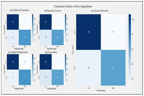
Figure 10.
Confusion Matrix of the Mentioned Algorithms.
Figure 10a–e correspond to the confusion matrix of the XGBoost classification algorithm, random forest algorithm, logistic regression algorithm, integration algorithm, and sequential model neural network algorithm, respectively. From the perspective of method type comparison, the left side of Figure 10 corresponds to a machine learning algorithm. The right side corresponds to a deep learning algorithm. Taking the confusion matrix of the sequential model neural network algorithm as an example, 107 in the first column of the first row indicates that 107 instances of the actual predicted ‘low’ traffic are correctly predicted as ‘low’ traffic. In the second column of the first row, 11 instances that actually belong to ‘low’ traffic are incorrectly predicted as ‘high’ traffic; the 18 in the first column of the second row indicates that the 18 instances that actually belong to the ‘high’ flow are predicted to be ‘low’ flow; and the 64 in the second column of the second row indicates that the 64 instances that actually belong to ‘high’ traffic are correctly predicted as ‘high’ traffic. Similarly, with reference to the above analysis methods, the true positive, false negative, false positive, and true negative indexes of XGBoost classification algorithm, random forest algorithm, logistic regression algorithm, and integrated algorithm can be analyzed from the confusion matrix.
In addition, more advanced classification indicators can be obtained from the confusion matrix: precision and recall. Precision is the most commonly used classification performance index. It can be used to represent the accuracy of the model, that is, the correct number/total number of samples identified by the model. Generally speaking, the higher the accuracy of the model, the better the effect of the model. The specific definition is as shown in Formula (13):
In addition, the definition of recall is as follows:
The recall rate, also known as sensitivity, measures the classifier’s ability to identify positive samples among the actual positive instances. Specifically, it is defined as the ratio of the number of positive samples accurately identified by the model to the total number of positive samples. Precision and recall are two conflicting metrics. Generally, when the precision is high, the recall tends to be low; conversely, when the recall is high, the precision often decreases. The precision and recall of the above five algorithms are shown in Figure 11:
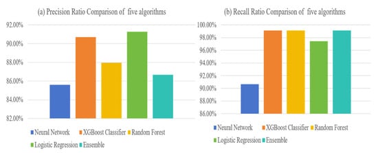
Figure 11.
The Recall Rate and Precision Rate of Five Algorithms.
As shown in Figure 11a,b, the precision rates of the sequential model neural network, XGBoost classification algorithm, random forest, logistic regression, and integrated model are 85.60%, 90.70%, 87.97%, 91.27%, and 86.67%, respectively, and the recall rates are 90.68%, 99.15%, 99.15%, 97.46%, and 99.15%, respectively. Among them, the logistic regression algorithm has the highest precision rate of 91.27%; the recall rate of XGB Classifier, random forest, and integrated model is the highest, which is 99.15%.
Next, the predictive values of the number of traffic occurrence instances on the test set are compared between the sequential model neural network algorithm and the integrated model, as shown in Figure 12:
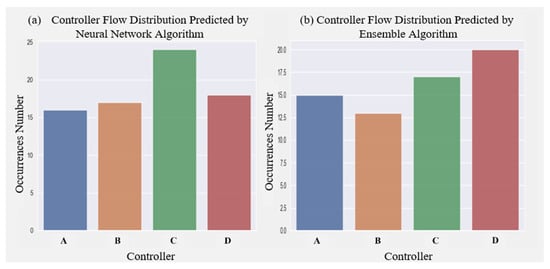
Figure 12.
Traffic Prediction of Sequential Model Neural Network and Ensemble Model on Test Set, Respectively.
Figure 12a,b describe the traffic prediction of the sequential model neural network algorithm and the ensemble algorithm on the test set, respectively. Comparing Figure 12a,b, it can be seen that the flow prediction on the C and D controllers is quite different. The predictive flow of the sequential model neural network for the C controller is 24 instances, and the predictive flow for the D controller is 18 instances. The prediction flow of the integrated algorithm for the C controller is 17 instances, and the prediction flow for the D controller is 20 instances. Network traffic prediction can provide a basis for judging the load balancing of a SDVN, and then provide a reference for the iterative update optimization of SDVN controller dynamic deployment. For the difference in traffic prediction results, we can further judge the prediction advantages and disadvantages of different algorithms when studying the dynamic deployment of SDVN controllers in the future.
4. Conclusions
This paper considers four factors when studying SDVN controller deployment: network traffic (network load), number of RSUs, RSU location, and delay. The deterministic annealing clustering algorithm is used to solve the model. After determining the number of SDVN controllers to be four, namely A, B, C, and D, the network traffic is further analyzed and predicted. In network traffic prediction, the sequential model neural network algorithm, XGBoost classifier algorithm, random forest algorithm, logistic regression algorithm, support vector machine algorithm, and ensemble algorithm are used. The average accuracy, standard deviation of accuracy, precision, and recall of the above algorithms are compared. Finally, the prediction differences between the integrated model and the neural network algorithm for the number of future traffic occurrences of A, B, C, and D controllers are compared. In the traffic prediction after the optimization of SDVN controller deployment, the performance of the machine learning algorithm is better than that of the neural network algorithm, because the judgment of network traffic is based on the binary classification of ‘high’ and ‘low’. In terms of the performance of the binary classification problem, machine learning algorithms are often not weaker than deep learning neural network algorithms.
Author Contributions
Conceptualization, H.L. (Hongming Li) and H.L. (Hao Li); methodology, H.L. (Hao Li) and H.L. (Hongming Li); software, H.L. (Hongming Li); validation, H.L. (Hao Li); formal analysis, H.L. (Hongming Li) and H.L. (Hao Li); investigation, H.L. (Hongming Li) and Y.J.; resources, H.L. (Hongming Li) and Y.J.; data curation, H.L. (Hongming Li), H.L. (Hao Li) and Z.W.; writing—original draft preparation, H.L. (Hao Li); writing—review and editing, H.L. (Hao Li), H.L. (Hongming Li), Y.J. and Z.W.; visualization, H.L. (Hongming Li) and Y.J.; supervision, H.L. (Hao Li) and Z.W.; project administration, H.L. (Hao Li); funding acquisition, H.L. (Hao Li). All authors have read and agreed to the published version of the manuscript.
Funding
This research was funded by the China Postdoctoral Science Foundation, grant number 2024M762090.
Institutional Review Board Statement
Not applicable.
Informed Consent Statement
Not applicable.
Data Availability Statement
The data presented in this study are available on request from the corresponding author. The data are not publicly available due to privacy.
Conflicts of Interest
The authors declare no conflicts of interest.
References
- Li, H.; Ji, Y.; Wang, Z. A New Hybrid Hierarchical Roadside Unit Deployment Scheme Combined with Parking Cars. Appl. Sci. 2024, 14, 7032. [Google Scholar] [CrossRef]
- Lee, E.K.; Gerla, M.; Pau, G.; Lee, U.; Lim, J.H. Internet of Vehicles: From intelligent grid to autonomous cars and vehicular fogs. Int. J. Distrib. Sens. Netw. 2016, 9. [Google Scholar] [CrossRef]
- Hussain, R.; Son, J.; Eun, H.; Kim, S.; Oh, H. Rethinking Vehicular Communications: Merging VANET with cloud computing. In Proceedings of the 4th IEEE International Conference on Cloud Computing Technology and Science Proceedings, Taipei, Taiwan, China, 3–6 December 2012; pp. 606–609. [Google Scholar] [CrossRef]
- Lee, E.; Lee, E.K.; Gerla, M.; Oh, S.Y. Vehicular cloud networking: Architecture and design principles. IEEE Commun. Mag. 2014, 52, 148–155. [Google Scholar] [CrossRef]
- Salahuddin, M.A.; Al-Fuqaha, A.; Guizani, M. Software-defined networking for rsu clouds in support of the internet of vehicles. IEEE Internet Things J. 2015, 2, 133–144. [Google Scholar] [CrossRef]
- Mershad, K.; Artail, H. Finding a STAR in a vehicular cloud. IEEE Intell. Transp. Syst. Mag. 2013, 5, 55–68. [Google Scholar] [CrossRef]
- Ang, L.; Jiayi, Y.; Detian, K.; Meng, M.Q.-H. Localization of Pedicle Screw Placement Plane Based on Reinforcement Learning. Procedia Comput. Sci. 2024, 250, 37–43. [Google Scholar] [CrossRef]
- Khojand, M.; Majidzadeh, K.; Farhang, M.Y. Controller placement in SDN using game theory and a discrete hybrid metaheuristic algorithm. J. Supercomput. 2024, 80, 6552–6600. [Google Scholar] [CrossRef]
- Heller, B.; Sherwood, R.; McKeown, N. The controller placement problem. ACM SIGCOMM Comput. Commun. Rev. 2012, 42, 473–478. [Google Scholar] [CrossRef]
- Wang, G.; Zhao, Y.; Huang, J.; Duan, Q.; Li, J. A K-means-based network partition algorithm for controller placement in software defined network. In Proceedings of the 2016 IEEE International Conference on Communications (ICC), Kuala Lumpur, Malaysia, 22–27 May 2016; pp. 1–6. [Google Scholar] [CrossRef]
- Zhao, J.; Qu, H.; Zhao, J.; Zhirong, L.; Guo, Y. Towards controller placement problem for software-defined network using affinity propagation. Electron. Lett. 2017, 53, 928–929. [Google Scholar] [CrossRef]
- Zhang, T.; Bianco, A.; Giaccone, P. The role of inter-controller traffic in SDN controllers placement. In Proceedings of the 2016 IEEE Conference on Network Function Virtualization and Software Defined Networks (NFV-SDN), Palo Alto, CA, USA, 7–10 November 2016; pp. 87–92. [Google Scholar] [CrossRef]
- Zeng, D.; Teng, C.; Gu, L.; Yao, H.; Liang, Q. Flow setup time aware minimum cost switch-controller association in Software-Defined Networks. In Proceedings of the 2015 11th International Conference on Heterogeneous Networking for QSHINE, Taipei, Taiwan, 19–20 August 2015; pp. 259–264. [Google Scholar] [CrossRef]
- Han, L.; Li, Z.; Liu, W.; Dai, K.; Qu, W. Minimum control latency of SDN controller placement. In Proceedings of the 2016 IEEE Trustcom/BigDataSE/ISPA, Tianjin, China, 23–26 August 2016; pp. 2175–2180. [Google Scholar] [CrossRef]
- Usmani, Z.; Singh, S. A Survey of Virtual Machine Placement Techniques in a Cloud Data Center. Phys. Procedia 2016, 78, 491–498. [Google Scholar] [CrossRef]
- Younis, M.; Akkaya, K. Strategies and techniques for node placement in wireless sensor networks: A survey. Ad. Hoc Netw. 2008, 6, 621–655. [Google Scholar] [CrossRef]
- Melo, M.T.; Nickel, S.; Saldanha-da-Gama, F. Facility location and supply chain management—A review. Eur. J. Oper. Res. 2009, 196, 401–412. [Google Scholar] [CrossRef]
- He, Y.; Zhao, N.; Yin, H. Integrated networking, caching, and computing for connected vehicles. A deep reinforcement learning approach. IEEE Trans. Veh. Technol. 2018, 67, 44–55. [Google Scholar] [CrossRef]
- Tootoonchian, A.; Ganjali, Y. HyperFlow: A distributed control plane for OpenFlow. In Proceedings of the NSDI Internet Network Management Workshop/Workshop on Research on Enterprise Networking (INM/WREN), San Jose, CA, USA, 27 April 2010. [Google Scholar]
- Koponen, T.; Amidon, K.; Balland, P.; Casado, M.; Chanda, A.; Fulton, B.; Ganichev, I.; Gross, J.; Gude, N.; Ingram, P.; et al. Network virtualization in multi-tenant datacenters. In Proceedings of the 11th USENIX Symposium on Networked Systems Design and Implementation (NSDI’14), Seattle, WA, USA, 2–4 April 2014; pp. 203–216. [Google Scholar]
- Vissicchio, S.; Vanbever, L.; Bonaventure, O. Opportunities and research challenges of hybrid software defined networks. Comput. Commun. Rev. 2014, 44, 70–75. [Google Scholar] [CrossRef]
- Hu, T.; Guo, Z.; Yi, P.; Baker, T.; Lan, J. Multi-controller Based Software-Defined Networking: A Survey. IEEE Access 2018, 6, 15980–15996. [Google Scholar] [CrossRef]
- Blial, O.; Ben Mamoun, M.; Benaini, R. An Overview on SDN Architectures with Multiple Controllers. J. Comput. Netw. Commun. 2016, 2016, 9396525. [Google Scholar] [CrossRef]
- Liao, J.; Sun, H.; Wang, J.; Qi, Q.; Li, K.; Li, T. Density cluster based approach for controller placement problem in large-scale software defined networkings. Comput. Netw. 2017, 112, 24–35. [Google Scholar] [CrossRef]
- Perrot, N.; Reynaud, T. Optimal placement of controllers in a resilient SDN architecture. In Proceedings of the 2016 12th International Conference on the Design of Reliable Communication Networks, DRCN 2016, Paris, France, 15–17 March 2016; pp. 145–151. [Google Scholar] [CrossRef]
- Naning, H.S.; Munadi, R.; Effendy, M.Z. SDN controller placement design: For large scale production network. In Proceedings of the 2016 IEEE Asia Pacific Conference on Wireless and Mobile (APWiMob), Bandung, Indonesia, 13–15 September 2016; pp. 74–79. [Google Scholar] [CrossRef]
- Lin, Q.; Zhang, D. Traffic-Aware compatible controller deployment. In Proceedings of the 2015 10th International Conference on Communications and Networking in China (ChinaCom), Shanghai, China, 15–17 August 2015; pp. 847–852. [Google Scholar] [CrossRef]
- Xiao, X.F.; Kui, X. The Characterizes of Communication Contacts Between Vehicles and Intersections for Software-Defined Vehicular Networks. Mob. Netw. Appl. 2015, 20, 98–104. [Google Scholar] [CrossRef]
- Deng, D.J.; Lien, S.Y.; Lin, C.C.; Hung, S.-C.; Chen, W.-B. Latency Control in Software-Defined Mobile-Edge Vehicular Networking. IEEE Commun. Mag. 2017, 55, 87–93. [Google Scholar] [CrossRef]
- Qin, Q.; Poularakis, K.; Iosifidis, G.; Kompella, S.; Tassiulas, L. SDN Controller Placement with Delay-Overhead Balancing in Wireless Edge Networks. IEEE Trans. Netw. Serv. Manag. 2018, 15, 1446–1459. [Google Scholar] [CrossRef]
- Han, M.; Fan, L. A short-term energy consumption forecasting method for attention mechanisms based on spatio-temporal deep learning. Comput. Electr. Eng. 2024, 114, 109063. [Google Scholar] [CrossRef]
- Rao, Z.; Xu, Y.; Pan, S.; Guo, J.; Yan, Y.; Wang, Z. Cellular Traffic Prediction: A Deep Learning Method Considering Dynamic Non-Local Spatial Correlation, Self-Attention, and Correlation of Spatio-Temporal Feature Fusion. IEEE Trans. Netw. Serv. Manag. 2022, 20, 426–440. [Google Scholar] [CrossRef]
- Palanisamy, T.; Sadayan, G.; Pathinetampadiyan, N. Neural network–based leaf classification using machine learning. Concurr. Comput. Pract. Exp. 2022, 34, e5366. [Google Scholar] [CrossRef]
Disclaimer/Publisher’s Note: The statements, opinions and data contained in all publications are solely those of the individual author(s) and contributor(s) and not of MDPI and/or the editor(s). MDPI and/or the editor(s) disclaim responsibility for any injury to people or property resulting from any ideas, methods, instructions or products referred to in the content. |
© 2025 by the authors. Licensee MDPI, Basel, Switzerland. This article is an open access article distributed under the terms and conditions of the Creative Commons Attribution (CC BY) license (https://creativecommons.org/licenses/by/4.0/).