Multi-Scale Feature Fusion and Global Context Modeling for Fine-Grained Remote Sensing Image Segmentation

Abstract

High-precision remote sensing image semantic segmentation plays a crucial role in Earth science analysis and urban management, especially in urban remote sensing scenarios with rich details and complex structures. In such cases, the collaborative modeling of global and local contexts is a key challenge for improving segmentation accuracy. Existing methods that rely on single feature extraction architectures, such as convolutional neural networks (i.e., CNNs) and vision transformers, are prone to semantic fragmentation due to their limited feature representation capabilities. To address this issue, we propose a hybrid architecture model called PLGTransformer, which is based on dual-encoder collaborative enhancement and integrates pyramid pooling and graph convolutional network (i.e., GCN) modules. Our model innovatively constructs a parallel encoding architecture combining Swin transformer and CNN: the CNN branch captures fine-grained features such as road and building edges through multi-scale heterogeneous convolutions, while the Swin transformer branch models global dependencies of large-scale land cover using hierarchical window attention. To further strengthen multi-granularity feature fusion, we design a dual-path pyramid pooling module to perform adaptive multi-scale context aggregation for both feature types and dynamically balance local and global contributions using learnable weights. Specifically, we introduce the GCNs to build a topological graph in the feature space, enabling geometric relationship reasoning for multi-scale feature nodes at high resolution. Experiments on the Potsdam and Vaihingen datasets show that our model outperforms contemporary advanced methods and significantly improves segmentation accuracy for small objects such as vehicles and individual buildings, thereby validating the effectiveness of the multi-feature collaborative enhancement mechanism.

1. Introduction

With revolutionary advancements in aerospace and sensor technologies, remote sensing data acquisition capabilities have achieved transformative breakthroughs. Researchers now have unprecedented access to multidimensional Earth observation systems comprising optical imagery, multispectral/hyperspectral data, synthetic aperture radar (SAR), and light detection and ranging (LiDAR) [1,2,3]. These cutting-edge datasets, featuring sub-meter spatial resolution, nanometer-level spectral resolution, and hourly temporal resolution, not only accurately document spatiotemporal evolution patterns of terrestrial ecosystems but also reveal profound spatial imprints of human activities [1,4,5]. Effectively mining valuable information from massive heterogeneous datasets has emerged as a critical scientific challenge in intelligent remote sensing interpretation.

The synergistic fusion of multisource remote sensing data establishes a new paradigm for Earth system science research. By integrating complementary sensor advantages, researchers can construct multidimensional feature spaces to enhance surface characterization capabilities. This paradigm demonstrates remarkable efficacy in change detection: SAR’s all-weather observation combined with optical spectral information enables precise urban expansion monitoring [1,3,4]; hyperspectral–LiDAR fusion elevates land cover classification accuracy beyond $90\%$ [6,7]; and multi-temporal multi-angle image integration effectively resolves camouflage recognition challenges in military applications [8,9]. These breakthroughs propel the paradigm shift from visual to intelligent interpretation in remote sensing [10,11,12,13].

As the core technology for deep image understanding, semantic segmentation has gained significant attention in remote sensing. Through pixel-level classification generating semantic thematic maps, it supports decision making in digital twin cities, flood assessment, and precision agriculture. However, unique remote sensing characteristics—sub-pixel features (e.g., small-scale structures), inter-class similarity (e.g., vegetation types), and target occlusion—pose formidable challenges to conventional segmentation algorithms [14,15,16,17]. Particularly in high-density urban areas, traditional CNNs (i.e., convolutional neural networks) struggle to distinguish occluded boundaries due to limited receptive fields, leading to significant accuracy degradation. These challenges drive research on novel segmentation frameworks tailored for remote sensing characteristics.

While CNN-based models excel in feature extraction, their hierarchical downsampling mechanisms progressively discard small-scale features. For instance, 3- to 5-pixel-wide road markings in high-resolution urban imagery degrade to sub-pixel levels after four downsampling operations, complicating network recognition. Furthermore, weakened inter-class heterogeneity (e.g., vegetation spectral confusion, similar reflectance between buildings and pavements) undermines the CNN’s reliance on local textures for establishing discriminative boundaries [15,18,19,20]. Combined with vertical occlusion effects, these limitations exacerbate pixel-level semantic ambiguity, highlighting the inadequacy of single-scale feature extraction.

To tackle these challenges, we focus on developing multi-granularity feature fusion systems that combine local details with global context. The Swin transformer [21] introduces hierarchical window attention mechanisms alongside CNN-style feature learning. It features: (1) progressive feature pyramids achieved through patch merging, (2) window-based multi-head self-attention (W-MSA) that reduces computational complexity, and (3) shifted window (SW-MSA) mechanisms that address limitations in the visual field. However, the limitations of transformers in weak boundaries (such as water–wetland transitions) and high-frequency textures (like farmland furrows) highlight the need for the local inductive bias of CNNs, which has prompted research into hybrid architectures [22]. Dual-branch networks that combine CNN and transformer pathways, along with channel-spatial attention mechanisms, show superior multimodal fusion capabilities. Building on these foundations, this paper proposes PLGTransformer—a dual-encoder-enhanced hybrid architecture that innovatively integrates local perception, global modeling, and graph-structured reasoning. Compared with existing hybrid CNN–transformer architectures such as Swin UNet and FTUNetFormer, PLGTransformer introduces several technical and structural innovations. Specifically, it employs a triple-branch heterogeneous CNN design to capture fine-grained and diverse local features, a dual-path pyramid self-learning fusion module (PSFM) with learnable weights for adaptive multi-scale fusion, and a novel graph fusion module (GFM) based on GCNs to model spatial topological relationships in high-dimensional feature space. These modules collaboratively improve semantic continuity, small object recognition, and long-range contextual understanding, addressing core limitations such as boundary fragmentation and semantic inconsistency in complex remote sensing scenes. To summarize, our main contributions include:

1.

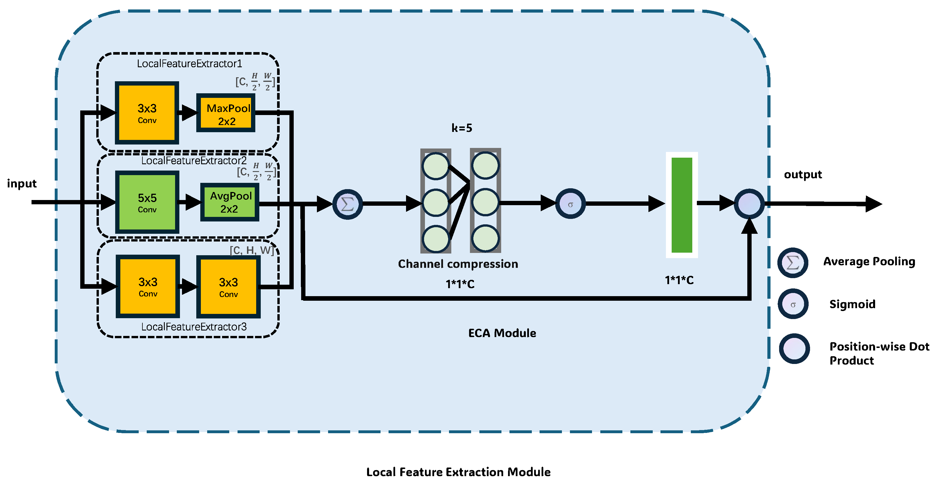
Heterogeneous Multi-Branch Local Feature Extraction: The proposed model establishes a multi-scale local feature extraction network through three parallel convolutional branches. Specifically, the feature extractors perform diverse processing operations within different architectures to better capture comprehensive representations such as high-frequency textures, mesoscale structures, and detail representations for the remote sensing images. By doing this, the aligned and concatenated composite features preserve both sub-pixel edge responses and regional semantic correlations, effectively addressing the feature representation limitations of single convolutional kernels.

2.

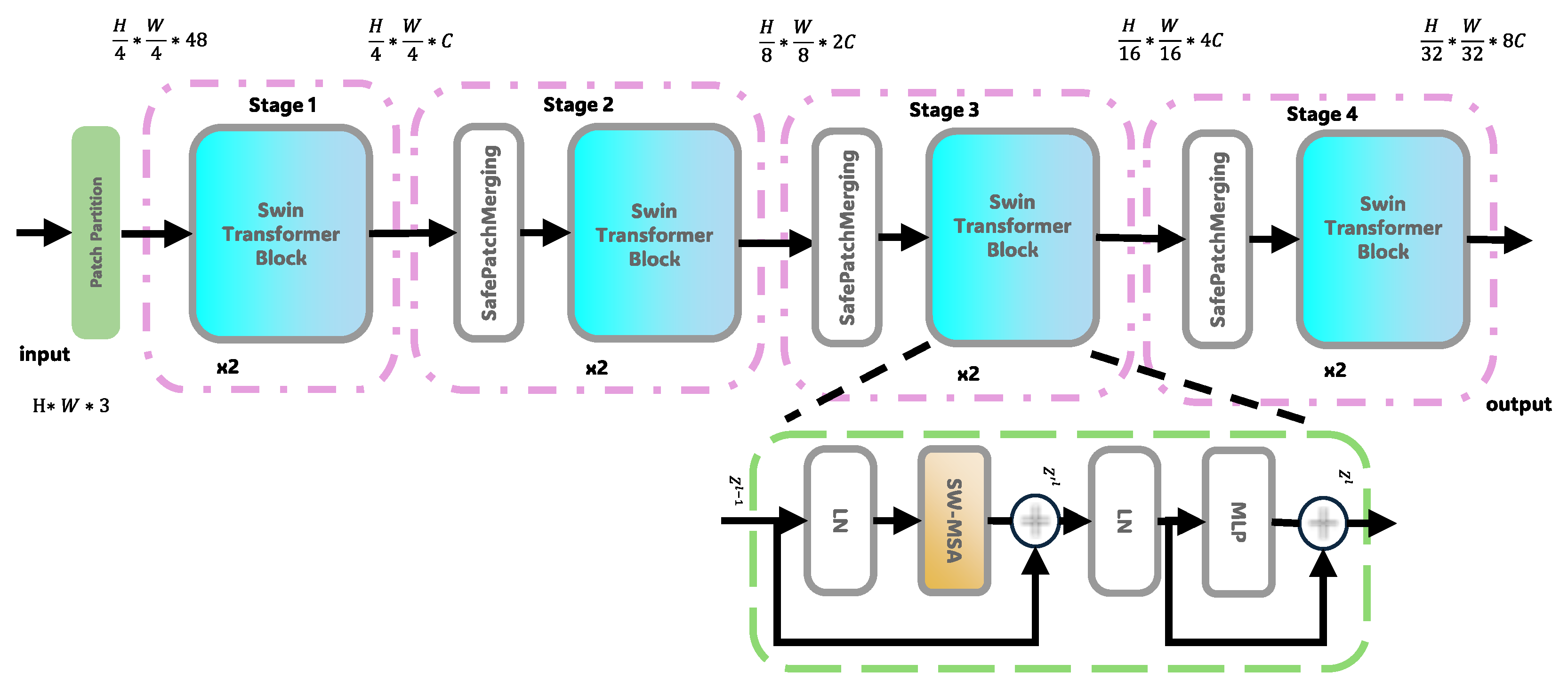
Hierarchical Window Attention with Pyramid Pooling: To mitigate the transformer’s local detail loss, we propose an enhanced customized architecture, termed the pyramid self-learning fusion module, by constructing four-level feature pyramids via patch merging. The dynamic shifted window mechanism enables cross-scale context modeling. Innovatively, dual pyramid pooling modules perform multi-granular spatial pooling on local and global features. After bilinear upsampling and convolution-based channel control, this strategy significantly improves vegetation classification by fusing local details with global semantics.

3.

Spatial Graph Convolution-Guided Feature Propagation: The proposed graph fusion module maps local, global, and fused features into high-dimensional graph nodes, constructing spatial topology using four-neighbor adjacency matrices. Three GCN pathways facilitate feature propagation, with learnable weights dynamically aggregating improved node features. This design goes beyond traditional grid limitations, establishing long-range dependencies in the reconstruction space to address semantic discontinuities caused by high-rise occlusions.

In the next section, we discuss some related works in remote sensing image segmentation. Subsequently, the proposed framework is detailed in Section 3, followed by a presentation of all experimental results in Section 4. Finally, in Section 5, we discuss future research directions and summarize this work.

2. Related Works

In recent years, deep-learning-based image segmentation techniques have made remarkable progress, with a core focus on effectively extracting and fusing multi-scale and multi-modal features. Representative technologies such as CNNs and transformers have propelled this field from the perspectives of local perception and global dependency modeling, respectively. Research trends are gradually shifting from single-model dominance toward hybrid approaches that integrate multiple techniques to overcome individual limitations and achieve performance breakthroughs.

2.1. CNN-Based Remote Sensing Image Segmentation

CNNs have achieved significant success in the field of remote sensing semantic segmentation due to their powerful capabilities in local feature extraction and spatial relationship modeling. Early CNN architectures like AlexNet [18] and VGGNet [23] achieved hierarchical abstraction of image features through stacked convolutional layers, laying the groundwork for subsequent remote sensing image analysis. The fully convolutional network (FCN) [24] replaced fully connected layers with convolutional layers to enable end-to-end pixel-level predictions, marking a milestone in remote sensing segmentation.

Building on the FCN framework, U-Net [25] introduced an encoder-decoder architecture with skip connections, effectively addressing the challenge of detail recovery in remote sensing images. This design enables the network to fuse low-level edge information with high-level semantic features during decoding, making it especially suited for accurately delineating complex object boundaries in remote sensing scenarios. The DeepLab series [26] further expanded the receptive field by introducing atrous convolution while preserving spatial resolution—crucial for capturing multi-scale features in remote sensing images. Notably, the atrous spatial pyramid pooling (ASPP) module in DeepLabV3+ effectively captures multi-scale contextual information, enhancing segmentation accuracy for objects of varying sizes. To address the unique characteristics of remote sensing imagery, Chen et al. [27] proposed a CNN model based on attention mechanisms that learns to weigh important features, thereby improving recognition of complex land covers. Wang et al. [28] introduced a multi-scale feature fusion strategy to effectively handle large variations in object scale within remote sensing data. However, traditional CNNs have limitations in modeling long-range dependencies, making it challenging to capture broad contextual and non-local features in remote sensing images. This has prompted researchers to explore more advanced model architectures.

2.2. Transformer-Based Remote Sensing Semantic Segmentation

Originally successful in natural language processing [29], transformers have since been adopted in computer vision. The vision transformer (ViT) [30] processes images as sequences of fixed-size patches to model global context but suffers from quadratic computational complexity relative to input image size, limiting its applicability to high-resolution remote sensing images. The Swin transformer alleviates this limitation by introducing a shifted window mechanism. Its hierarchical structure and localized self-attention computation allow for global dependency modeling while maintaining linear computational complexity, making it especially suitable for large-scale remote sensing images. The Swin transformer’s ability to represent multi-scale features enables outstanding performance in remote sensing segmentation tasks, particularly in modeling extensive regions and intricate textures. He et al. [31] proposed Swin-UNet, which integrates the Swin transformer into a U-Net framework, combining transformer-based global modeling with U-Net’s detailed feature recovery. Xu et al. [32] developed a hierarchical feature extraction network based on the Swin transformer to address multi-scale semantic segmentation in remote sensing images. Bazi et al. [33] designed the RS-ST model specifically for high-resolution remote sensing imagery, incorporating improved window partitioning and feature fusion strategies to enhance sensitivity to complex boundaries. Liu et al. [34] further incorporated a spatial attention module into the Swin transformer, improving the model’s perception of spatial distribution patterns in remote sensing data. Despite their strength in modeling long-range dependencies, transformers still face challenges in capturing fine-grained local details, motivating research into hybrid architectures that combine CNNs and transformers to leverage their complementary strengths.

2.3. GCN-Based and Other Related Deep Learning Methods

GCNs [35] perform convolutions in non-Euclidean space, offering a new paradigm for processing data with complex topological structures. In remote sensing segmentation, GCNs can effectively model spatial relationships and contextual dependencies between objects, addressing the limitations of CNNs’ local receptive fields. Remote sensing imagery often exhibits complex spatial dependencies. Liang et al. [36] applied GCNs to remote sensing segmentation by constructing pixel-level relational graphs, enhancing spatial correlation modeling—which is particularly beneficial for segmenting irregularly shaped objects. Chen et al. [37] proposed a dynamically constructed GCN model that adaptively connects nodes based on feature similarity, improving segmentation accuracy in complex scenes. Sun et al. [38] innovatively combined GCNs with attention mechanisms to design a spatial-relationship-enhanced network, learning long-range dependencies between objects to significantly improve segmentation performance. Zhang et al. [39] further explored multi-scale graph convolution operations, constructing graphs at different scales to improve recognition of objects of varying sizes. In recent years, the integration of CNNs, transformers, and GCNs has become a research hotspot. Wang et al. [40] proposed a hybrid architecture where CNNs extract local features, transformers model global dependencies, and GCNs enhance spatial relationship modeling—together significantly improving remote sensing segmentation accuracy. Li et al. [41] designed a hierarchical feature fusion framework that applies CNNs, transformers, and GCNs at different levels, achieving more accurate boundary delineation through multi-level feature complementarity. Our proposed PLGTransformer model follows this trend by integrating the strengths of CNNs (local feature extraction), Swin transformers (global context modeling), and GCNs (spatial relationship enhancement) into a unified remote sensing segmentation framework. This model effectively handles multi-scale features and complex textures in remote sensing images while modeling spatial dependencies through graph structures, thus achieving more accurate and robust semantic segmentation results.

With the growth of deep learning technologies, research is increasingly focused on improving feature extraction and modeling in remote sensing image segmentation. The Mamba model [42], an emerging deep learning architecture, has shown promise in this area. It combines convolutional neural networks (CNN) with attention mechanisms, enabling effective local feature extraction and global dependency modeling. This allows the Mamba model to distinguish objects in complex images and handle multi-scale features, making it particularly effective for high-resolution remote sensing images with varying object sizes [43]. Additionally, the Mamba model enhances segmentation performance through multimodal information fusion, utilizing data from different sensors such as optical and radar images. This capability improves object recognition and segmentation accuracy in complex environments [44]. Overall, the Mamba model excels in remote sensing image segmentation, leveraging CNNs and attention mechanisms to provide effective solutions across various applications.

The YOLO (you only look once) model [45] is a deep-learning-based object detection method recognized for its efficient real-time processing capabilities. Initially designed for object detection, YOLO has gained attention in remote sensing image segmentation due to its end-to-end training, which allows it to learn effective image features automatically. YOLO divides images into grids, with each grid predicting the location and category of objects, enabling the detection and segmentation of multiple targets in a single pass. This approach is more efficient than traditional sliding window techniques, especially for large-area remote sensing images. Its rapid detection makes YOLO suitable for real-time applications, such as disaster monitoring and urban planning, where it can quickly identify land cover changes. For instance, Gao et al. [46] applied YOLO in flood monitoring to swiftly pinpoint affected areas. However, while YOLO excels in object detection, it may lack precision in complex segmentation tasks requiring high detail, prompting researchers to enhance it by integrating other deep learning techniques for better accuracy.

Long short-term memory (LSTM) [47] networks are a type of recurrent neural network (RNN) designed for handling long-term dependencies in sequential data. Originally developed for language models and time series, LSTMs have proven effective in remote sensing image segmentation due to their ability to capture time- or space-varying patterns. They are particularly useful for processing multi-temporal remote sensing data, allowing models to learn relationships between images from different time points and detect land cover changes. For example, Chen et al. [48] applied LSTM to monitor urban development and crop growth, accurately identifying land cover changes. However, LSTMs require substantial training data and computational resources, which can limit their practical application, especially for high-resolution images. Nevertheless, advancements in technology are enhancing the feasibility of LSTM models in remote sensing image segmentation, particularly for tasks needing high spatiotemporal resolution.

3. Methodology

This section details the overall design of our proposed PLGTransformer model, including its parallel encoding architecture and graph convolutional fusion module. The model integrates multi-scale feature representation with local spatial cues, global contextual information, and graph-structured awareness, significantly improving semantic segmentation performance.

3.1. Overall Architecture

The overall architecture of PLGTransformer is illustrated in Figure 1. The model combines the strengths of CNNs for local structural perception, the Swin transformer for global dependency modeling, and GCNs for structured spatial representation. This synergy enables accurate segmentation of multi-scale and diverse land cover types in remote sensing imagery. The PLGTransformer comprises three main functional modules.

First, three heterogeneous local feature extractors are employed in parallel to extract multi-scale local representations, enhancing the model’s ability to capture texture and boundary information. Second, a hierarchical Swin transformer backbone is used to model global context through shifted window-based multi-head self-attention, efficiently capturing long-range dependencies. Third, pyramid pooling modules are embedded into both local and global branches to broaden semantic perception and enhance contextual awareness via multi-scale pooling. After local and global features are extracted, a learnable weighted fusion mechanism is designed to explicitly integrate these complementary sources, optimizing the combination of heterogeneous features. Furthermore, a graph-based fusion module is introduced to enhance spatial structure awareness. This module leverages GCNs to model topological relationships within the fused features, strengthening spatial adjacency and boundary continuity.

Finally, a convolutional prediction head and an upsampling module map the refined feature maps back to the original input resolution, yielding pixel-wise semantic segmentation outputs. In summary, PLGTransformer adopts a three-level synergy of local–global–structural design, forming an end-to-end segmentation framework with both multi-scale understanding and spatial modeling capabilities for remote sensing applications.

3.2. Parallel Encoding Architecture

We achieve efficient local feature extraction and multi-scale contextual fusion through the collaborative design of a heterogeneous convolutional architecture and pyramid pooling. Specifically, as shown in Figure 2, three independent local feature extractors—LocalFeatureExtractor1, LocalFeatureExtractor2, and LocalFeatureExtractor3—each use convolutional kernels of different sizes for feature extraction and optimize the features through pooling strategies. This can be expressed as follows:

(1) LocalFeatureExtractor1:

$${feat}_1=MaxPool2d\left({Conv2d}_{3\times 3}\left(x\right)\right).$$

(1)

Here, a $3\times 3$ convolutional kernel (i.e., ${Conv2d}_{3\times 3}$) is used to extract high-frequency texture features from the input x, and the max pooling (i.e., $MaxPool2d$) operation retains prominent features.

(2) LocalFeatureExtractor2:

$${feat}_2=AvgPool2d\left({Conv2d}_{5\times 5}\left(x\right)\right).$$

(2)

A 5 × 5 convolutional kernel is used to extract mid-scale semantic features, and the average pooling (i.e., $AvgPool2d$) operation suppresses noise.

(3) LocalFeatureExtractor3:

$${feat}_3={Conv2d}_{3\times 3}\left(x\right)·{Conv2d}_{3\times 3}\left(x\right).$$

(3)

The cascading of two $3\times 3$ convolutional kernels is used to extract fine-grained detail features. After feature extraction through the three branches, the features are upsampled to a $64\times 64$ resolution using bilinear interpolation and concatenated along the channels to obtain a unified local feature map:

$$local\_features=Concat({feat}_1,{feat}_2,{feat}_3).$$

(4)

Figure 2. The architecture of the local feature extractor in the parallel feature encoder.

Figure 2. The architecture of the local feature extractor in the parallel feature encoder.

To achieve efficient long-range dependency modeling and global feature extraction, we use an improved hierarchical Swin transformer and enhance global feature modeling through dynamic window attention mechanisms. As shown in Figure 3, the input image is first divided into non-overlapping image patches using a $4\times 4$ convolution kernel in the patch embedding layer, generating a 96-channel feature map of size $H/4\times W/4$. The image is then input into the four-stage transformer architecture. In the first stage, it contains two Swin blocks, using a fixed window size of $8\times 8$ for multi-head attention calculation (four heads). This stage enhances the low-level semantic representation through the interaction of local and global features:

$$stage1\_out={SwinBlock}_1\left({SwinBlock}_2\left(patches\right)\right)$$

(5)

Then, from the second to fourth stages, a hierarchical downsampling strategy is adopted, where the SafePatchMerging module merges adjacent $2\times 2$ feature blocks before each stage, achieving $2\times$ downsampling of spatial resolution ($H/8\to H/16\to H/32$) and a stepwise expansion of channel numbers. The mathematical expressions are:

$$stage2\_out=SafePatchMerging\left(stage1\_out\right).$$

(6)

$$stage3\_out=SafePatchMerging\left(stage2\_out\right).$$

(7)

$$stage4\_out=SafePatchMerging\left(stage3\_out\right).$$

(8)

Each Swin block uses an alternating structure of window multi-head attention and shifted window attention, which is represented as:

$$Attention(Q,K,V)=Softmax\left({\displaystyle \frac{Q{K}^T}{\sqrt{d_k}}}+B\right)V,$$

(9)

where B is a learnable relative positional bias and $d_k$ is the dimension of each attention head. To obtain the attention matrices, we perform linear projections on the input features $X\in {\mathbb{R}}^{B\times N\times C}$, where B is the batch size, N is the number of tokens, and C is the channel dimension. These subspaces represent queries (Q), keys (K), and values (V) through learned projection matrices:

$$Q=X{W}^Q,K=X{W}^K,V=X{W}^V,$$

(10)

where $W^Q$, $W^K$, and $W^V\in {\mathbb{R}}^{C\times d_k}$ are learnable projection matrices. The dot-product between Q and K determines the attention weights, and these weights are applied to V to perform a weighted aggregation of features within each window. This enables the model to selectively attend to semantically relevant regions.

During the merging, features from $2\times 2$ neighboring regions are concatenated and projected through a linear layer for downsampling and channel expansion. The final global feature output is normalized and upsampled via bilinear interpolation to align with the local feature resolution.

3.3. Pyramid Self-Learning Fusion Module

To effectively capture multi-scale contextual information in images and enhance the segmentation ability for complex objects, we propose an adaptive pyramid pooling fusion module, as shown in Figure 4. This module optimizes feature fusion through multi-scale context aggregation and dynamic weight learning. The specific design is as follows:

(1) Pyramid Pooling Operation: The module first applies the pyramid pooling operation to both local and global feature channels to extract contextual information at different scales. Specifically, for the input feature map $x_k$, we perform pooling at different scales:

$${pyramid\_feat}_k=AvgPool\left(x_k\right)w.r.tk\in \{1,2,3,\dots \},$$

(11)

where $x_k$ denotes the feature maps at different pooling scales.

(2) Feature Dimension Matching: To reduce the number of channels and match the feature dimensions, the multi-scale features obtained from pooling are processed through a $1\times 1$ convolution:

$${pool\_feat}_k=Conv2d({pyramid\_feat}_k,{channels}_{out}),$$

(12)

where ${channels}_{out}$ is the output number of channels after the convolution.

(3) Feature Concatenation and Weighted Fusion: The pooled multi-scale features are fused through concatenation:

$$fused\_feat=Concat({pool\_feat}_1,{pool\_feat}_2,\dots ).$$

(13)

Subsequently, we design a weighted fusion mechanism, which explicitly fuses local and global features through a 1 × 1 convolution and learnable normalized weights:

$$fused\_output=Conv2d\left(fused\_feat\right)·Softmax\left(weights\right),$$

(14)

where $weights$ are the normalized weights learned to dynamically adjust the contribution ratios from different feature sources. This mechanism can dynamically adjust the contribution of different feature sources based on the task requirements, thus improving the expression ability of fused features, enhancing the network’s perception of features at different scales, and ultimately improving the accuracy and robustness of semantic segmentation for remote sensing images.

Figure 4. The main structure of the pyramid self-learning fusion module.

Figure 4. The main structure of the pyramid self-learning fusion module.

3.4. Graph Fusion Module

While CNNs and transformers effectively extract local and global features, they face challenges in capturing structured spatial relationships—particularly in complex remote sensing scenes. Pixels in remote sensing images exhibit not only local attributes but also long-range, structured dependencies tied to object boundaries, textures, shapes, and inter-object interactions. To better model such spatial structures, we introduce a Graph Fusion Module based on GCNs. This module enhances the semantic coherence and boundary accuracy of the segmentation results by learning topological relations across multi-source features. As shown in Figure 5, the multi-source graph convolution fusion network constructs dynamic graphs and learns adaptive weights to model the topological relationships between local and global features. The specific design process is as follows:

(1) Graph Construction: The module constructs a multi-adjacency graph structure, converting local features, global features, and fused features into graph nodes, and performs graph convolution operations to enhance the expression of target boundaries, structural relationships, and spatial consistency. First, the local, global, and fused features are uniformly upsampled to generate feature maps:

$$\text{feature\_map}=\text{UpSample}(\text{local\_features},\text{global\_features},\text{fused\_features}).$$

(15)

These feature maps are flattened to form the node feature matrix H and the adjacency matrix A.

(2) Graph Convolution Operation: The graph convolution operation updates the node features H as follows:

$$H^{\prime }=\sigma \left(D^{-1/2}A{D}^{-1/2}HW\right),$$

(16)

where D is the degree matrix, A is the adjacency matrix, W is the learnable weight matrix, and $\sigma$ is the activation function. Here, the adjacency matrix $A\in {\mathbb{R}}^{N\times N}$ is constructed using dot-product attention between each pair of nodes to capture the semantic similarity among spatial regions. The degree matrix D is a diagonal matrix where each element $D_{ii}$ represents the sum of the i-th row of A, i.e., $D_{ii}={\sum }_j{A}_{ij}$. The graph convolution operation is performed separately on local features, global features, and fused features. This formulation allows information to propagate across semantically related but spatially distant regions, which is especially beneficial in high-resolution remote sensing imagery.

(3) Weighted Fusion: A learnable vector $\gamma =[{\gamma }_1,{\gamma }_2,{\gamma }_3]$ is used to perform weighted fusion on the graph convolution outputs of local, global, and fused features:

$$\text{fused\_output}={\gamma }_1{H}_{\mathrm{local}}^{\prime }+{\gamma }_2{H}_{\mathrm{global}}^{\prime }+{\gamma }_3{H}_{\mathrm{fused}}^{\prime }.$$

(17)

The weights ${\gamma }_1$, ${\gamma }_2$, and ${\gamma }_3$ are initialized equally and normalized using a softmax function during training to ensure numerical stability and interpretability. This adaptive fusion mechanism enables the model to dynamically emphasize the most informative source according to different scene contexts or object categories.

(4) Category Mapping and Feature Recovery: Finally, the network maps the fused output to the category space using a $1\times 1$ convolution and recovers the features to the input size using bilinear interpolation, thus obtaining the final semantic prediction map:

$$\text{pred\_map}=\mathrm{BilinearInterpolation}\left({\mathrm{Conv}}_{1\times 1}\left(\text{fused\_output}\right)\right).$$

(18)

This process is simple and efficient, supports end-to-end training, and is particularly suitable for segmentation tasks in remote sensing images with complex structures and diverse scales.

Figure 5. The main structure of the graph fusion module.

Figure 5. The main structure of the graph fusion module.

3.5. Loss Function

In remote sensing image semantic segmentation, precise object recognition requires high accuracy in both region classification and boundary localization. This is crucial for high-resolution images, where complex object shapes can lead to blurred boundaries and concentrated errors. This study presents a composite loss function, the Multi-scale Boundary Focal Loss Function, to optimize both region recognition and boundary delineation. This loss function consists of two components: the first component is the Multi-class Region Focal Loss, which is used to optimize pixel-wise classification within regions; the second component is the multi-scale boundary loss, which strengthens the model’s sensitivity to boundary pixels. The final combined loss function is expressed as follows:

$$L_{total}=(1-\beta )·L_{region}+\beta ·L_{boundary}$$

(19)

where $L_{region}$ denotes the multi-class region focal loss for the region, $L_{boundary}$ represents the multi-scale boundary loss, and $\beta$ is the balancing coefficient controlling the relative importance of the two components. Among them, the two loss terms are defined as:

$$L_{region}={\alpha }_{\mathrm{region}}·{(1-p_{true})}^{\gamma }·log\left(p_{true}\right)$$

(20)

$$L_{boundary}={\displaystyle \frac{1}{N_{scales}}}\sum _{s=1}^{N_{scales}}\mathrm{BCEWithLogitsLoss}(p_{foreground}^s,{\text{boundary\_mask}}^s)$$

(21)

The number of classes is set to six, addressing the requirements of multi-class segmentation tasks in remote sensing images. For the multi-class region focal loss, the focusing parameter $\gamma$ is set to 2.0 to emphasize hard examples, and the class balancing factor ${\alpha }_{\mathrm{region}}$ is set to 1.0 to ensure equal treatment across all categories. The multi-scale boundary loss introduces a separate coefficient ${\alpha }_{\mathrm{boundary}}$, which is set to 0.3 to increase the model’s sensitivity to boundary pixels. To enhance boundary awareness across spatial resolutions, this loss is computed over three different scales: $0.5\times$, $1.0\times$, and $2.0\times$ of the original size. Finally, the coefficient $\beta$ is empirically set to 0.3, balancing the influence of regional classification and boundary localization in the final loss.

4. Experiments and Discussion

The primary objective of the experiments is to quantitatively and qualitatively verify the performance of the proposed model in remote sensing image segmentation. By comparing with traditional methods and the latest deep learning models, we aim to demonstrate the advantages of the proposed model in improving segmentation accuracy, handling boundaries, and detecting small objects.

4.1. Dataset Descriptions

In this study, we used the ISPRS Vaihingen and Potsdam datasets to evaluate the PLGTransformer model. Both datasets contain high-resolution remote sensing images and digital surface models (DSM), providing detailed label information for semantic segmentation tasks.

• Vaihingen Dataset: The Vaihingen dataset consists of 16 high-resolution orthophotos, each measuring $2500\times 2000$ pixels. Each image includes three spectral channels: near-infrared (NIR), red (R), and green (G), along with a DSM at 9 cm ground sampling distance (GSD). The dataset includes five foreground classes (buildings, trees, low vegetation, cars, and impervious surfaces) and one background class (clutter). In our experiments, 12 images were used for training and 4 for testing, following a commonly used protocol. Additionally, 20% of the training samples were randomly selected as a validation set. All images were divided into non-overlapping $256\times 256$ patches for training and evaluation.
• Potsdam Dataset: The Potsdam dataset contains 24 orthophotos with a resolution of $6000\times 6000$ pixels, and four spectral channels: red (R), green (G), blue (B), and infrared (IR), at 5 cm GSD. It shares the same class definitions as the Vaihingen dataset. We adopted the same patch generation and training/validation strategy as used in Vaihingen, with an 80/20% split for training and testing, and 20% of training samples used for validation.

4.2. Experimental Setup

All experiments were implemented on an GeForce RTX 4090 GPU, NVIDIA, Macao SAR, China, using the PyTorch framework with 24 GB RAM. The specific setup is as follows: We used the AdamW optimizer with an initial learning rate of 0.0001, momentum of 0.9, a decay factor of 0.0005, and a sliding window size of 256 × 256 for training. During testing, the sliding window size was 32. Data augmentation methods like random rotation, horizontal flipping, and vertical flipping were employed. The training duration was set to 100 epochs.

The AdamW optimizer performed excellently in image segmentation tasks, particularly during deep network training. To avoid overfitting, L2 regularization (weight decay) was added during training with a weight decay coefficient of 1 $\times {10}^{-4}$. The learning rate was dynamically adjusted using the CosineAnnealingLR scheduler to help the model converge more effectively. The batch size was set to four, and we also implemented dropout and early stopping mechanisms to prevent overfitting. Validation metrics like IoU and F1-Score were monitored, and training was stopped early when no improvement was observed.

We utilized custom loss functions such as multi-scale boundary loss and adaptive focal loss. The multi-scale boundary loss helped the model better handle boundary regions, while the adaptive focal loss addressed class imbalance by adjusting the weight of each class dynamically.

4.3. Evaluation Metrics

In this experiment, we used multiple evaluation metrics to measure the model’s segmentation performance. Common evaluation metrics for remote sensing image segmentation include intersection over union (IoU) and F1 score.

• IoU (Intersection over Union): IoU is a standard metric for evaluating image segmentation model performance, calculated as the intersection area of the predicted and ground truth regions divided by their union area. A higher IoU indicates better segmentation accuracy. In the experiments, we computed the IoU for each class and averaged them to obtain the overall IoU. A high IoU value indicates that the model performs well in handling complex boundaries and small objects.
• F1 Score: F1 score is the harmonic mean of precision and recall and is typically used to evaluate models with class imbalance. In remote sensing image segmentation tasks, some classes may have significantly fewer samples than others. The F1 score provides a more comprehensive evaluation of the model’s performance across different object types. A higher F1 score indicates better balance between precision and recall.

To evaluate the segmentation results from multimodal remote sensing data, we used the mean F1 score (mF1) and mean IoU (mIoU) as the key statistical indicators. These metrics were used to compare the performance of the proposed PLGTransformer with other state-of-the-art methods. Specifically, we computed mF1 and mIoU for the four foreground classes and averaged them to get the final results.

4.4. Comparative Experiments

We compare the PLGTransformer with several state-of-the-art remote sensing image segmentation methods on two different datasets. The selected models for comparison include SwinT [21], Swin UNet [49], BANet [50], FTUNetFormer [51], and CTFuse [52]. As shown in

Table 1. Comparison results of different modules on the Vaihingen dataset.

Model	Imp. Surf. (%)		Building (%)		Car (%)		Low Veg. (%)		Tree (%)		mIoU (%)	mF1 (%)
	IoU	F1	IoU	F1	IoU	F1	IoU	F1	IoU	F1
SwinT	72.74	82.27	81.90	88.83	26.24	44.02	66.31	79.93	68.41	79.46	63.12	74.90
Swin UNet	65.75	77.08	71.51	81.24	28.05	46.36	55.10	69.61	61.01	73.89	56.28	69.64
BANet	72.14	81.87	81.47	88.44	32.96	52.26	65.70	79.38	68.94	79.84	64.24	76.36
FTUNetFormer	75.91	84.60	84.49	90.38	43.71	63.99	69.06	82.33	70.28	80.88	68.69	80.44
CTFuse	77.19	85.37	78.51	87.96	56.06	71.84	73.20	84.53	72.03	83.74	71.40	82.69
PLGTransformer	81.46	88.45	77.64	87.41	59.05	74.26	73.38	84.65	72.74	84.22	72.85	83.80

, on the Vaihingen dataset, the PLGTransformer achieves performance scores of $72.85\%$ for mean intersection over union (mIoU) and $83.80\%$ for mean F1 score (mF1). Compared to the baseline model CTFuse, PLGTransformer improves by $1.45\%$ in mIoU and $1.11\%$ in mF1. The table highlights that our model excels in the categories of impermeable surfaces, buildings, low vegetation, and trees. Figure 6 presents the visual results obtained by all six methods on the Vaihingen dataset.

On the Potsdam dataset, as shown in

Table 2. Comparison results of different models on the Potsdam dataset.

Model	Imp. Surf. (%)		Building (%)		Car (%)		Low Veg. (%)		Tree (%)		mIoU (%)	mF1 (%)
	IoU	F1	IoU	F1	IoU	F1	IoU	F1	IoU	F1
SwinT	65.17	74.50	58.06	63.03	51.71	58.41	67.84	79.01	58.74	68.76	60.30	68.74
Swin UNet	59.52	69.56	54.59	60.22	56.77	62.52	63.38	75.12	52.06	62.35	57.26	65.95
BANet	63.25	72.82	55.99	61.28	53.51	59.82	66.77	78.09	54.65	64.62	58.83	67.33
FTUNetFormer	66.87	75.78	59.23	63.96	57.66	63.24	70.16	81.14	60.25	70.30	62.83	70.88
CTFuse	67.98	76.55	68.81	81.52	59.56	74.66	77.46	87.30	61.37	76.06	67.04	79.22
PLGTransformer	58.90	74.14	85.21	92.01	70.44	82.66	61.11	70.40	75.14	85.81	70.16	81.00

, the PLGTransformer achieves performance scores of $70.16\%$ for mean intersection over union (mIoU) and $81.00\%$ for mean F1 score (mF1). Compared to the baseline model CTFuse, PLGTransformer improves by $3.12\%$ in mIoU and $1.78\%$ in mF1. Figure 7 presents the visual results obtained by all six methods on the Potsdam dataset. Similar to the results on the Vaihingen dataset, our PLGTransformer performs better than other state-of-the-art models in handling fine details.

It is evident that, compared to other state-of-the-art models, our PLGTransformer performs better in recognizing fine details and handling edges. Specifically, the CNN + Swin transformer parallel encoding structure effectively combines local texture information with global semantic context, providing a stronger receptive field and region discrimination ability. As observed in Figure 6, the dual-branch encoding structure allows the model to maintain clear boundary expressions when processing complex scenes, such as “building-road” and “building-low vegetation” adjacent areas. Moreover, the pyramid self-learning fusion module (PSFM) in the decoding stage adapts and guides the fusion of multi-scale features, allowing the model to flexibly focus on important regions at different scales. The model effectively captures the subtle semantic transitions between buildings and surrounding low vegetation, achieving continuous edges and complete form segmentation of building objects, significantly outperforming other comparison methods. The integrated GFM models structural relationships between objects in the high-level semantic space, enhancing semantic consistency and reducing errors like object fragmentation. In conclusion, the proposed model excels in segmentation accuracy and shows superior generalization in structural continuity, boundary completeness, and small object recognition.

To further validate the training process and convergence behavior of the proposed model, we continuously monitored the loss values on both the training and validation sets throughout the optimization process. Figure 8 illustrates the training-validation loss curves on the Vaihingen and Potsdam datasets. The blue curve represents the training loss, while the orange curve corresponds to the validation loss. As shown in the figure, both losses exhibit a consistent downward trend and tend to stabilize after approximately the 60th epoch, indicating that the model successfully converges without showing signs of severe overfitting. Moreover, the validation loss closely follows the trend of the training loss, further demonstrating the strong generalization capability of the proposed PLGTransformer on two distinct remote sensing datasets.

In our study, all experiments were conducted using an GeForce RTX 4090 GPU, NVIDIA, Macao SAR, China, with 24GB of memory, implemented under the PyTorch 1.12.0 framework. For a standard input size of $256\times 256$, the batch size was set to 4, and the model achieved an average inference time of approximately 0.018 s per image, with an average memory usage of around 484 MB. During the testing phase, we employed a $32\times 32$ sliding window strategy to perform tiled inference on large-scale images, effectively controlling memory consumption while preserving spatial continuity.

4.5. Ablation Experiments

4.5.1. Performance Analysis from Different Modules

To validate the effectiveness of each component in the PLGTransformer, we conducted a series of ablation experiments. By retaining the dual-branch framework, we removed specific components to assess their contributions. We used the basic CNN + Swin transformer as the baseline and performed ablation experiments on both datasets for comparison. We separately removed the pyramid self-learning fusion module (PSFM) and the graph neural network fusion module (GFM) on the two datasets. Compared with the baseline dual-encoder model, the full PLGTransformer demonstrated consistent accuracy gains after integrating the PSFM and GFM modules. When the pyramid self-learning fusion module (PSFM) was removed, the model’s performance significantly dropped, especially in tasks involving the segmentation of small objects and fine details. For instance, in the Vaihingen dataset, the IoU for the “car” category increased from 18.05% in the baseline model to 59.05% in the full model, clearly illustrating PSFM’s strong ability in enhancing fine-grained representations and local spatial cues. This demonstrates that shallow feature fusion is crucial for preserving local details such as object shapes and boundaries.When the graph neural network fusion module (GFM) was removed, the model’s ability to model global contextual information significantly decreased. Deep feature fusion plays a key role in handling long-range dependencies and spatial continuity in high-resolution RGB imagery. Specifically, the “tree” category in the Potsdam dataset showed a marked IoU improvement from 41.01% to 75.14% in the full model, indicating the GFM’s effectiveness in modeling spatial relationships and semantic coherence within single-modality RGB features. Figure 9 presents the performance of different modules in the ablation experiments.

The Vaihingen dataset contains images with high texture complexity and a significant presence of small objects, such as vehicles, and densely distributed targets, such as buildings. The experimental results, as shown in

Table 3. Ablation results from different modules on the Vaihingen dataset.

Model	Imp. Surf. (%)		Building (%)		Car (%)		Low Veg. (%)		Tree (%)		mIoU (%)	mF1 (%)
	IoU	F1	IoU	F1	IoU	F1	IoU	F1	IoU	F1
Base	65.75	77.08	71.51	81.24	18.05	26.36	45.10	59.61	61.01	73.89	52.29	63.64
Base+PSFM	67.28	78.41	78.70	86.81	6.90	11.24	50.68	64.70	61.90	74.27	53.09	63.09
Base+GFM	70.57	80.66	79.66	87.19	29.19	39.27	53.71	67.62	67.07	78.35	60.04	70.62
Base+PSFM+GFM	81.46	88.45	77.64	87.41	59.05	74.26	73.38	84.65	72.74	84.22	72.85	83.80

, are as follows. After removing the PSFM module, the overall accuracy of the model significantly decreased, with mIoU dropping from $72.85\%$ to $60.04\%$ and mF1 decreasing from $83.80\%$ to $70.62\%$. This performance drop was particularly noticeable in the recognition of “small object” categories. Notably, the car IoU dropped by $29.86\%$, emphasizing the PSFM’s contribution to small-object localization and edge preservation. The introduction of the PSFM played a key role in multi-scale feature fusion and boundary recovery, especially improving performance in the “building” and “low vegetation” categories. When the GFM module was removed, the model’s performance in handling large-scale scenes declined, with both mIoU and mF1 values dropping. The mIoU decreased from $72.85\%$ to $53.09\%$, and there was a noticeable blurring of boundaries in large-scale scenes, highlighting the crucial role of GFM in modeling global contextual information. In remote sensing images, land cover objects often exhibit spatial dependencies over long distances. The GFM effectively captures such relationships through topological reasoning over the fused RGB features, without relying on cross-modal fusion. This is particularly evident in categories such as “tree”, where boundary continuity and spatial consistency are vital for accurate classification. The complete model (base + PSFM + GFM) achieved the best performance on this dataset, with significant improvements over the baseline. After integrating the PSFM and GFM, the model’s accuracy was balanced in both small object and large area segmentation, demonstrating the model’s ability to optimize both global and local features in a collaborative manner.

The Potsdam dataset, known for its high resolution and diverse categories, is ideal for model performance evaluation. The experimental results in

Table 4. Ablation results from different modules on the Potsdam dataset.

Model	Imp. Surf. (%)		Building (%)		Car (%)		Low Veg. (%)		Tree (%)		mIoU (%)	mF1 (%)
	IoU	F1	IoU	F1	IoU	F1	IoU	F1	IoU	F1
Base	59.52	69.56	59.72	64.58	40.61	45.91	52.27	63.12	41.01	51.08	50.63	58.85
Base+PSFM	61.18	71.40	76.76	82.10	42.35	50.52	61.87	73.26	61.00	70.97	60.63	69.65
Base+GFM	62.26	72.06	75.00	80.57	56.55	62.58	58.73	70.19	65.70	76.22	63.65	72.32
Base+PSFM+GFM	58.90	74.14	85.21	92.01	70.44	82.66	61.11	70.40	75.14	85.81	70.16	81.00

indicate that removing the PSFM reduces mIoU from $70.16\%$ to $63.65\%$, significantly impairing small object segmentation, notably for “car” categories, where IoU drops by $13.89\%$. This again demonstrates that the PSFM is particularly beneficial for enhancing fine-scale structure and small object boundaries in RGB-based segmentation. Removing the GFM further decreases mIoU to $60.63\%$, highlighting its importance for large-scale semantic classification and maintaining global structural consistency. The “tree” and “building” categories, for instance, exhibit more fragmented and spatially incoherent predictions when the GFM is removed. The combined removal of both modules results in a $9.53\%$ IoU decrease and an $11.35\%$ F1 drop. Using both PSFM and GFM together markedly improves the handling of complex structures, enhancing feature fusion and spatial consistency in challenging RGB scenes.

The visual results presented in Figure 10 further validate the quantitative findings discussed above. PSFM exhibits outstanding performance in small object detection and multi-scale scenarios, effectively preserving object shapes and contours even in cases with blurred boundaries. GFM plays a critical role in global semantic modeling, enhancing semantic consistency and capturing long-range dependencies, although its impact is slightly less pronounced compared to PSFM. The complete PLGTransformer model integrates both local and global information streams, resulting in improved segmentation accuracy and better generalization across datasets. Together, the quantitative and visual results demonstrate that both modules are essential for remote sensing image segmentation and exhibit strong functional complementarity.

4.5.2. Performance Variations on Diverse Losses

To evaluate the contribution of each component within the loss function, we conducted a series of ablation experiments on the Vaihingen dataset using our proposed PLGTransformer model. To better understand the role of each component, we designed the following experimental settings: (1) baseline—both multi-class region focal loss (i.e., $L_{region}$) and multi-scale boundary loss (i.e., $L_{boundary}$) are applied; (2) multi-class region focal loss only—only the multi-class region focal loss is used; (3) multi-scale boundary loss only—only the multi-scale boundary loss is used. The experimental results are summarized in

Table 5. Ablation results on the Vaihingen dataset with different loss settings. ✔ indicates the specific loss is added.

Setting	${\mathit{L}}_{\mathbf{region}}$	${\mathit{L}}_{\mathbf{boundary}}$	mIoU (%)	mF1 (%)
Baseline	✔	✔	72.85	83.80
Multi-Class Region Focal Loss Only	✔		61.62	70.09
Multi-Scale Boundary Loss Only		✔	63.43	74.06

. The experimental results show that the complete loss combination, which jointly optimizes both the region focal and boundary losses, results in the best overall performance. Removing either branch leads to a significant decrease in both mIoU and mF1 scores, demonstrating the complementary nature of region classification and boundary modeling.

4.5.3. Parameter Sensitivity Study on Compound Loss

In the ablation experiments, we confirmed the complementary nature of the region classification loss and the boundary modeling loss. To further examine the impact of their relative weighting within the combined loss function, we conducted a parameter sensitivity analysis on the Vaihingen dataset. This analysis aims to evaluate how different configurations influence the model’s segmentation performance and to identify the optimal balance between regional and boundary supervision. We examined four key parameters: (1) ${\alpha }_{\mathrm{region}}$, which is the weight for the region focal loss; (2) $\beta$, the balance coefficient between region and boundary losses; (3) $\gamma$, the focusing parameter in the focal loss; and (4) ${\alpha }_{\mathrm{boundary}}$, the weight for the boundary-specific loss term.

In each experiment, one parameter was varied across five representative values while fixing the others to their default configuration (${\alpha }_{\mathrm{region}}=1.0$, $\beta =0.3$, $\gamma =2.0$, ${\alpha }_{\mathrm{boundary}}=0.3$). The evaluation metrics include mean intersection over union (mIoU) and mean F1 score (mF1) on the validation set. As shown in

Table 6. Parameter sensitivity analysis of the compound loss on the Vaihingen dataset.

Parameter Varied	Value	Fixed Parameters	mIoU (%)	mF1 (%)
${\alpha }_{\mathrm{region}}$	0.25	$\beta =0.3$, $\gamma =2.0$, ${\alpha }_{\mathrm{boundary}}=0.3$	71.63	82.57
	0.5	$\beta =0.3$, $\gamma =2.0$, ${\alpha }_{\mathrm{boundary}}=0.3$	72.80	84.02
	1.0	$\beta =0.3$, $\gamma =2.0$, ${\alpha }_{\mathrm{boundary}}=0.3$	72.85	83.80
	2.0	$\beta =0.3$, $\gamma =2.0$, ${\alpha }_{\mathrm{boundary}}=0.3$	72.62	83.66
	5.0	$\beta =0.3$, $\gamma =2.0$, ${\alpha }_{\mathrm{boundary}}=0.3$	71.54	81.44
$\beta$	0.1	${\alpha }_{\mathrm{region}}=1.0$, $\gamma =2.0$, ${\alpha }_{\mathrm{boundary}}=0.3$	67.25	77.05
	0.3	${\alpha }_{\mathrm{region}}=1.0$, $\gamma =2.0$, ${\alpha }_{\mathrm{boundary}}=0.3$	72.85	83.80
	0.5	${\alpha }_{\mathrm{region}}=1.0$, $\gamma =2.0$, ${\alpha }_{\mathrm{boundary}}=0.3$	71.98	82.79
	0.7	${\alpha }_{\mathrm{region}}=1.0$, $\gamma =2.0$, ${\alpha }_{\mathrm{boundary}}=0.3$	68.64	76.55
	0.9	${\alpha }_{\mathrm{region}}=1.0$, $\gamma =2.0$, ${\alpha }_{\mathrm{boundary}}=0.3$	64.26	75.96
$\gamma$	0.0	${\alpha }_{\mathrm{region}}=1.0$, $\beta =0.3$, ${\alpha }_{\mathrm{boundary}}=0.3$	71.64	82.57
	1.0	${\alpha }_{\mathrm{region}}=1.0$, $\beta =0.3$, ${\alpha }_{\mathrm{boundary}}=0.3$	72.45	83.68
	2.0	${\alpha }_{\mathrm{region}}=1.0$, $\beta =0.3$, ${\alpha }_{\mathrm{boundary}}=0.3$	72.85	83.80
	3.0	${\alpha }_{\mathrm{region}}=1.0$, $\beta =0.3$, ${\alpha }_{\mathrm{boundary}}=0.3$	72.51	83.69
	5.0	${\alpha }_{\mathrm{region}}=1.0$, $\beta =0.3$, ${\alpha }_{\mathrm{boundary}}=0.3$	71.76	82.61
${\alpha }_{\mathrm{boundary}}$	0.1	${\alpha }_{\mathrm{region}}=1.0$, $\beta =0.3$, $\gamma =2.0$	71.12	81.92
	0.2	${\alpha }_{\mathrm{region}}=1.0$, $\beta =0.3$, $\gamma =2.0$	72.20	82.88
	0.3	${\alpha }_{\mathrm{region}}=1.0$, $\beta =0.3$, $\gamma =2.0$	72.85	83.80
	0.5	${\alpha }_{\mathrm{region}}=1.0$, $\beta =0.3$, $\gamma =2.0$	71.78	82.41
	1.0	${\alpha }_{\mathrm{region}}=1.0$, $\beta =0.3$, $\gamma =2.0$	70.50	80.75

, the model is relatively insensitive to ${\alpha }_{\mathrm{region}}$ and $\gamma$, maintaining stable performance across a wide range of values. In contrast, it is mildly sensitive to $\beta$, with noticeable performance degradation when deviating from the balanced setting of $\beta =0.3$. For ${\alpha }_{\mathrm{boundary}}$, the best performance is observed when it is set to 0.3. Increasing its value disrupts region classification, while reducing it weakens boundary clarity. This configuration achieves the best performance, consistent with the configuration used in the main experiments.

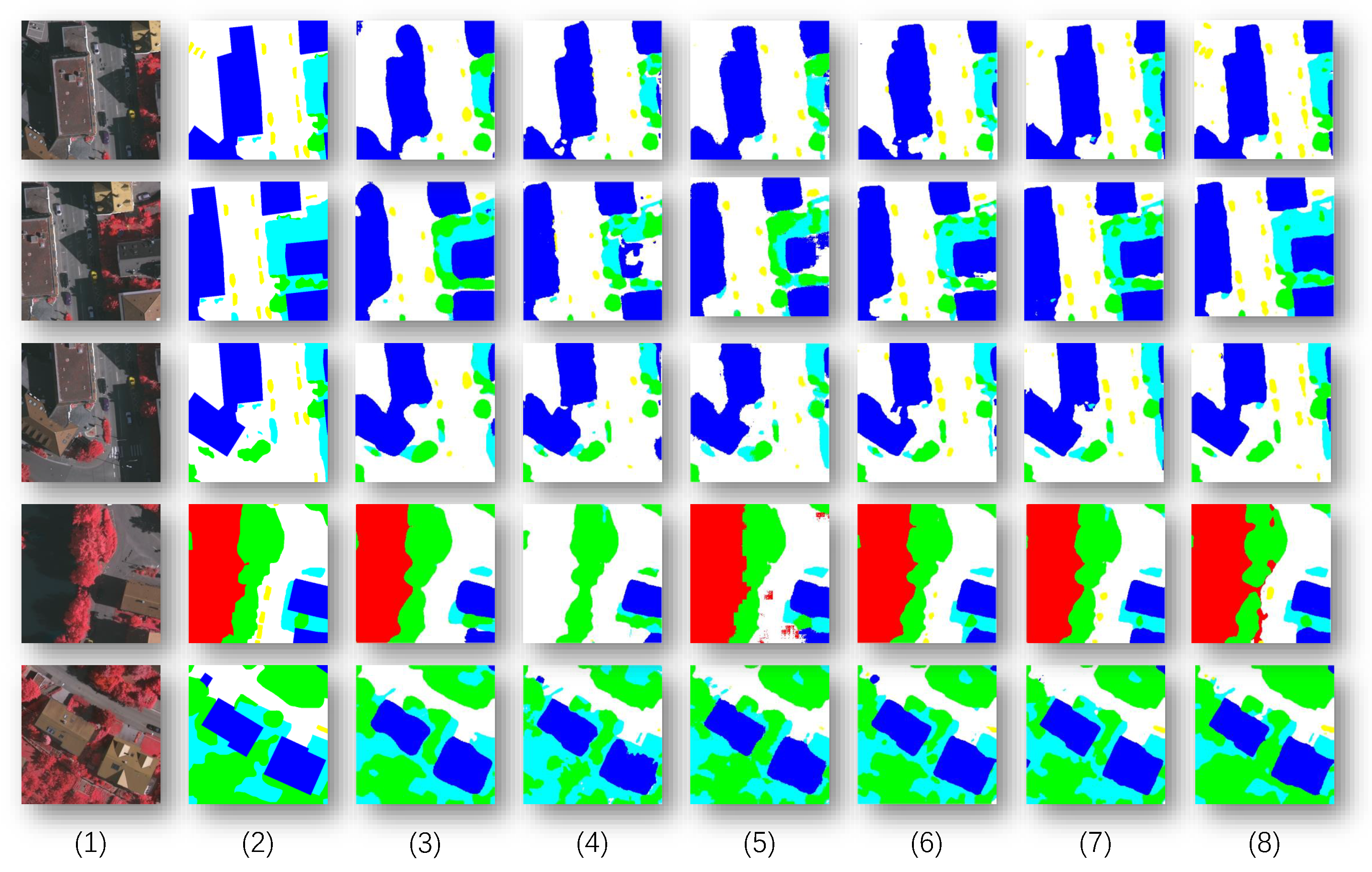
4.5.4. Visualization Analysis

To further validate the feature information that the PLGTransformer model focuses on in a specific convolutional layer, the Grad-CAM [53] method can be applied. Grad-CAM utilizes the gradients with respect to the target class to generate a heatmap by computing the weighted sum of the feature maps from the last convolutional layer. This method creates a weighted combination of the feature maps, where the weights correspond to the importance of each feature map for the classification decision. This heatmap highlights the regions of the image that contribute the most to the predicted class.

As shown in Figure 11, in the building class, the model mainly focuses on the locations of buildings in the image. In the low vegetation class, the model focuses on sparse vegetation areas. In the impervious surface class, the model focuses on the hard-covered ground areas. This demonstrates that Grad-CAM can effectively visualize the key regions of interest, helping to explain the model’s classification decisions.

4.6. Discussion

PLGTransformer integrates the advantages of convolutional neural networks (CNNs) and vision transformers, achieving outstanding performance in remote sensing image segmentation tasks. Specifically, the CNN backbone is responsible for capturing local fine-grained features, while the transformer module models global contextual dependencies and long-range interactions. This multi-level feature fusion mechanism enables PLGTransformer to effectively handle complex scenes and objects with rich structural details.

Although PLGTransformer demonstrates excellent accuracy in remote sensing segmentation, it still faces challenges in distinguishing certain categories, particularly trees and low vegetation. These classes often exhibit high similarity in color, texture, and shape, with blurred boundaries, posing difficulties for fine-grained discrimination. Currently, the model mainly relies on adaptive graph fusion and boundary-aware loss for edge modeling, without explicitly incorporating traditional edge detection algorithms like Canny, Sobel, or post-processing methods like conditional random fields (CRFs). In future work, we plan to investigate integrating classical edge detection results as auxiliary supervision signals, or incorporating lightweight post-processing modules as plugins to enhance boundary discrimination.

Moreover, despite its superior segmentation accuracy, PLGTransformer has relatively high computational complexity, particularly when processing high-resolution images. Memory consumption and inference time are considerably longer. Thus, optimizing the architecture to reduce computational and memory costs remains an important direction. Future research may delve into model compression for real-time applications, quantization techniques, or more efficient attention mechanisms, as well as lightweight models tailored for large-scale data processing.

Multimodal data fusion remains a vital area of research in remote sensing semantic segmentation. Although existing studies that combine multiple data types, such as optical imagery and DSM, have demonstrated improved separability for certain land cover categories, they also highlight challenges, including modality heterogeneity, spatial misalignment, and inconsistent feature representations [54,55,56,57]. In future work, we aim to incorporate diverse remote sensing modalities into the PLGTransformer framework, and design more adaptive cross-modal fusion mechanisms to mitigate the aforementioned issues and enhance model generalizability and robustness in complex scenarios involving SAR or LiDAR.

Finally, the design philosophy of PLGTransformer also holds potential for applications in fields such as medical image analysis and autonomous driving, where segmentation tasks often involve complex boundaries and multi-scale structures. However, the characteristics of data and task requirements differ significantly across domains, and thus model structure and training strategies need to be specifically adapted. Future studies will explore these directions to achieve effective cross-domain deployment and generalization.

5. Conclusions

This study proposes a novel semantic segmentation method for remote sensing images, named PLGTransformer, which integrates the strengths of convolutional neural networks (CNNs) and transformer architectures. It is designed to address the challenges of segmenting remote sensing imagery characterized by structural complexity and land-cover diversity. By constructing a multi-level and multi-scale feature fusion mechanism, the model effectively combines local detail extraction with global contextual understanding, thereby enhancing semantic expressiveness while maintaining boundary clarity. In the experimental section, we conducted a comprehensive evaluation on two public remote sensing datasets, ISPRS Vaihingen and Potsdam, using only RGB optical imagery. Experimental results demonstrate that PLGTransformer outperforms state-of-the-art methods across multiple mainstream evaluation metrics, exhibiting notable robustness and accuracy, particularly in complex classes such as buildings, trees, and impervious surfaces. The main contribution of this study lies in the introduction of a multi-resolution feature integration strategy that fuses shallow and deep semantics, along with the hierarchical window-based attention mechanism of the Swin transformer, which effectively models long-range dependencies. This design significantly enhances the model’s ability to perceive complex spatial patterns in remote sensing imagery.

PLGTransformer holds considerable potential for future extension. First, at the data level, modalities such as DSM, SAR, or LiDAR can be incorporated to design more sophisticated cross-modal feature fusion mechanisms, thereby improving performance in areas with complex terrain or occlusions. Second, considering similar segmentation demands in fields like medical imaging and autonomous driving, PLGTransformer demonstrates promising transferability. Future work could focus on adapting the model in terms of input modalities, architecture modifications, and inference efficiency for specific tasks. Lastly, to meet the high-resolution, large-scale, and real-time processing requirements in real-world remote sensing applications, lightweight model design, accelerated inference methods, and efficient sliding window segmentation strategies will be essential directions for further research.

References

1. Fu, K.; Lu, W.X.; Liu, X.Y.; Deng, C.B.; Yu, H.F.; Sun, X. A comprehensive survey and assumption of remote sensing foundation modal. Natl. Remote Sens. Bull. 2024, 28, 1667–1680. [Google Scholar] [CrossRef]
2. Yuan, T.; Hu, B. REU-Net: A Remote Sensing Image Building Segmentation Network Based on Residual Structure and the Edge Enhancement Attention Module. Appl. Sci. 2025, 15, 3206. [Google Scholar] [CrossRef]
3. He, Y.; Seng, K.P.; Ang, L.M.; Peng, B.; Zhao, X. Hyper-CycleGAN: A New Adversarial Neural Network Architecture for Cross-Domain Hyperspectral Data Generation. Appl. Sci. 2025, 15, 4188. [Google Scholar] [CrossRef]
4. Zhang, L.P.; Zhang, L.F.; Du, B. Deep Learning for Remote Sensing Data: A Technical Tutorial on the State of the Art. IEEE Geosci. Remote Sens. Mag. 2016, 4, 22–40. [Google Scholar] [CrossRef]
5. Kazerouni, A.; Karimijafarbigloo, S.; Azad, R.; Velichko, Y.; Bagci, U.; Merhof, D. FuseNet: Self-Supervised Dual-Path Network For Medical Image Segmentation. In Proceedings of the 2024 IEEE International Symposium on Biomedical Imaging (ISBI), Athens, Greece, 27–30 May 2024; pp. 1–5. [Google Scholar]
6. Radford, A.; Kim, J.W.; Hallacy, C.; Ramesh, A.; Goh, G.; Agarwal, S.; Sastry, G.; Askell, A.; Mishkin, P.; Clark, J.; et al. Learning Transferable Visual Models from Natural Language Supervision. In Proceedings of the International Conference on Machine Learning, Salt Lake City, UT, USA, 18–24 July 2021. [Google Scholar]
7. Yuan, L.; Chen, D.; Chen, Y.L.; Codella, N.C.F.; Dai, X.; Gao, J.; Hu, H.; Huang, X.; Li, B.; Li, C.; et al. Florence: A New Foundation Model for Computer Vision. arXiv 2021, arXiv:2111.11432. [Google Scholar]
8. Bao, H.; Dong, L.; Piao, S.; Wei, F. BEiT: BERT PreTraining of Image Transformers. In Proceedings of the The Tenth International Conference on Learning Representations, Vienna, Austria, 25–29 April 2022. [Google Scholar]
9. Sherrah, J. Fully convolutional networks for dense semantic labelling of high-resolution aerial imagery. arXiv 2016, arXiv:1606.02585. [Google Scholar]
10. Guo, Y.; Jia, X.; Paull, D. Effective sequential classifier training for SVM-based multitemporal remote sensing image classification. IEEE Trans. Image Process. 2018, 27, 3036–3048. [Google Scholar] [CrossRef]
11. Pal, M. Random forest classifier for remote sensing classification. Int. J. Remote Sens. 2007, 26, 217–222. [Google Scholar] [CrossRef]
12. Li, Y.; Zhang, Y. A New Paradigm of Remote Sensing Image Interpretation by Coupling Knowledge Graph and Deep Learning. Geomat. Inf. Sci. Wuhan Univ. 2022, 47, 1176–1190. [Google Scholar] [CrossRef]
13. Zhang, S.; Wu, G.; Gu, J.; Han, J. Pruning convolutional neural networks with an attention mechanism for remote sensing image classification. Electronics 2020, 9, 1209. [Google Scholar] [CrossRef]
14. Dong, R.; Pan, X.; Li, F. DenseU-net-based semantic segmentation of small objects in urban remote sensing images. IEEE Access 2019, 7, 65347–65356. [Google Scholar] [CrossRef]
15. Zhou, X.; Wu, G.; Sun, X.; Hu, P.; Liu, Y. Attention-Based Multi-Kernelized and Boundary-Aware Network for image semantic segmentation. Neurocomputing 2024, 597, 127988. [Google Scholar] [CrossRef]
16. Sun, X.; Chen, C.; Wang, X.; Dong, J.; Zhou, H.; Chen, S. Gaussian dynamic convolution for efficient single-image segmentation. IEEE Trans. Circuits Syst. Video Technol. 2021, 32, 2937–2948. [Google Scholar] [CrossRef]
17. Li, Z.; Wu, G.; Liu, Y. Prototype Enhancement for Few-Shot Point Cloud Semantic Segmentation. In Proceedings of the International Conference on Algorithms and Architectures for Parallel Processing, Macau, China, 29–31 October 2024; Springer: Berlin/Heidelberg, Germany, 2024; pp. 270–285. [Google Scholar]
18. Krizhevsky, A.; Sutskever, I.; Hinton, G.E. ImageNet classification with deep convolutional neural networks. In Proceedings of the NIPS, Red Hook, NY, USA, 3–6 December 2012; pp. 1097–1105. [Google Scholar]
19. An, W.; Wu, G. Hybrid spatial-channel attention mechanism for cross-age face recognition. Electronics 2024, 13, 1257. [Google Scholar] [CrossRef]
20. Lv, Q.; Sun, X.; Chen, C.; Dong, J.; Zhou, H. Parallel complement network for real-time semantic segmentation of road scenes. IEEE Trans. Intell. Transp. Syst. 2021, 23, 4432–4444. [Google Scholar] [CrossRef]
21. Liu, Z.; Lin, Y.; Cao, Y.; Hu, H.; Wei, Y.; Zhang, Z.; Lin, S.; Guo, B. Swin Transformer: Hierarchical vision transformer using shifted windows. In Proceedings of the ICCV, Montreal, QC, Canada, 10–17 October 2021; pp. 10012–10022. [Google Scholar]
22. Wan, Y.; Zhou, D.; Wang, C.; Liu, Y.; Bai, C. Multi-scale medical image segmentation based on pixel encoding and spatial attention mechanism. Sheng Wu Yi Xue Gong Cheng Xue Za Zhi 2024, 41, 511–519. [Google Scholar] [CrossRef]
23. Simonyan, K.; Zisserman, A. Very deep convolutional networks for large-scale image recognition. In Proceedings of the ICLR, San Diego, CA, USA, 7–9 May 2015. [Google Scholar]
24. Long, J.; Shelhamer, E.; Darrell, T. Fully convolutional networks for semantic segmentation. In Proceedings of the CVPR, Boston, MA, USA, 7–12 June 2015; pp. 3431–3440. [Google Scholar]
25. Ronneberger, O.; Fischer, P.; Brox, T. U-Net: Convolutional networks for biomedical image segmentation. In Proceedings of the MICCAI, Munich, Germany, 5–9 October 2015; pp. 234–241. [Google Scholar]
26. Chen, L.C.; Zhu, Y.; Papandreou, G.; Schroff, F.; Adam, H. Encoder-decoder with atrous separable convolution for semantic image segmentation. In Proceedings of the ECCV, Munich, Germany, 8–14 September 2018; pp. 801–818. [Google Scholar]
27. Chen, Y.; Wang, Y.; Jiao, P.; Feng, M. A self-attention CNN for remote sensing image semantic segmentation. IEEE Trans. Geosci. Remote Sens. 2021, 59, 3155–3169. [Google Scholar] [CrossRef]
28. Wang, Q.; Liu, S.; Chanussot, J.; Li, X. Scene classification with recurrent attention of VHR remote sensing images. IEEE Trans. Geosci. Remote Sens. 2019, 57, 1155–1167. [Google Scholar] [CrossRef]
29. Vaswani, A.; Shazeer, N.; Parmar, N.; Uszkoreit, J.; Jones, L.; Gomez, A.N.; Kaiser, Ł.; Polosukhin, I. Attention is all you need. In Proceedings of the NIPS, Long Beach, CA, USA, 4–9 December 2017; pp. 5998–6008. [Google Scholar]
30. Dosovitskiy, A.; Beyer, L.; Kolesnikov, A.; Weissenborn, D.; Zhai, X.; Unterthiner, T.; Dehghani, M.; Minderer, M.; Heigold, G.; Gelly, S.; et al. An image is worth 16x16 words: Transformers for image recognition at scale. In Proceedings of the Proc. ICLR, Vienna, Austria, 4 May 2021. [Google Scholar]
31. He, X.; Zhou, Y.; Zhao, J.; Zhang, D.; Yao, R.; Xue, Y. Swin transformer embedding UNet for remote sensing image semantic segmentation. IEEE Trans. Geosci. Remote Sens. 2022, 60, 1–15. [Google Scholar] [CrossRef]
32. Xu, Y.; Du, B.; Zhang, L. Multi-scale spatial context-aware transformer for remote sensing image segmentation. IEEE Trans. Geosci. Remote Sens. 2022, 60, 1–12. [Google Scholar]
33. Bazi, Y.; Bashmal, L.; Al Rahhal, M.M.; Dayil, R.A.; Ajami, N. Vision transformers for remote sensing image classification. Remote Sens. 2021, 13, 516. [Google Scholar] [CrossRef]
34. Liu, C.; Wu, H.; Li, Y.; Li, X. SwinFCN: A spatial attention Swin transformer backbone for semantic segmentation of high-resolution aerial images. Remote Sens. 2022, 14, 1075. [Google Scholar] [CrossRef]
35. Kipf, T.N.; Welling, M. Semi-supervised classification with graph convolutional networks. In Proceedings of the 5th International Conference on Learning Representations (ICLR 2017), Toulon, France, 24–26 April 2017. [Google Scholar]
36. Liang, J.; Deng, Y.; Zeng, D. A deep neural network combined CNN and GCN for remote sensing scene classification. IEEE J. Sel. Top. Appl. Earth Obs. Remote Sens. 2020, 13, 4325–4338. [Google Scholar] [CrossRef]
37. Chen, Z.; Badrinarayanan, V.; Lee, C.Y.; Rabinovich, A. GradNet: Gradient-guided network for visual object tracking. In Proceedings of the ICCV, Seoul, Republic of Korea, 27 October–2 November 2019; pp. 6162–6171. [Google Scholar]
38. Sun, F.; Li, W.; Guan, X.; Liu, H.; Wu, J.; Gao, Y. Dual attention graph convolutional network for semantic segmentation of very high resolution remote sensing imagery. IEEE Trans. Geosci. Remote Sens. 2022, 60, 1–14. [Google Scholar]
39. Zhang, Z.; Wang, L.; Zhang, Y. Multi-scale graph convolutional network for remote sensing image segmentation. IEEE Geosci. Remote Sens. Lett. 2022, 19, 1–5. [Google Scholar]
40. Wang, X.; Girshick, R.; Gupta, A.; He, K. Non-local neural networks. In Proceedings of the CVPR, Salt Lake City, UT, USA, 18–22 June 2018; pp. 7794–7803. [Google Scholar]
41. Li, Z.; Luo, Y.; Wang, Z.; Zhang, B. MAT-GCN: A multi-scale attention guided graph convolutional network for remote sensing scene classification. IEEE Trans. Geosci. Remote Sens. 2022, 60, 1–12. [Google Scholar]
42. Gu, A.; Dao, T. Mamba: Linear-Time Sequence Modeling with Selective State Spaces. arXiv 2023, arXiv:2312.00752. [Google Scholar]
43. Liu, M.; Dan, J.; Lu, Z.; Yu, Y.; Li, Y.; Li, X. CM-UNet: Hybrid CNN-Mamba UNet for Remote Sensing Image Semantic Segmentation. arXiv 2024, arXiv:2405.10530. [Google Scholar]
44. Zhang, Q.; Li, Z.; Xu, H. Multimodal fusion for remote sensing image segmentation using Mamba model. J. Appl. Remote Sens. 2022, 16, 19–32. [Google Scholar] [CrossRef]
45. Redmon, J.; Divvala, S.; Girshick, R.; Farhadi, A. You Only Look Once: Unified, Real-Time Object Detection. In Proceedings of the 2016 IEEE Conference on Computer Vision and Pattern Recognition (CVPR), Boston, MA, USA, 7–12 June 2015; pp. 779–788. [Google Scholar]
46. Gao, Y.; Liu, Z.; Zhang, X. Real-time remote sensing image change detection using YOLO. J. Remote Sens. Technol. 2019, 20, 89–101. [Google Scholar]
47. Vennerød, C.; Kjærran, A.; Bugge, E. Long Short-term Memory RNN. arXiv 2021, arXiv:2105.06756. [Google Scholar]
48. Chen, J.; Zhang, Y.; Liu, Q. Remote sensing image segmentation based on LSTM for urban change detection. Int. J. Remote Sens. 2020, 41, 2048–2061. [Google Scholar]
49. Cao, H.; Wang, Y.; Chen, J.; Jiang, D.; Zhang, X.; Tian, Q.; Wang, M. Swin-Unet: Unet-like Pure Transformer for Medical Image Segmentation. In Proceedings of the ECCV Workshops, Milan, Italy, 29 September–4 October 2021. [Google Scholar]
50. Chen, Y.; Lin, G.; Li, S.; Bourahla, O.E.; Wu, Y.; Wang, F.; Feng, J.; Xu, M.; Li, X. BANet: Bidirectional Aggregation Network With Occlusion Handling for Panoptic Segmentation. In Proceedings of the 2020 IEEE/CVF Conference on Computer Vision and Pattern Recognition (CVPR), Seattle, WA, USA, 13–19 June 2020; pp. 3792–3801. [Google Scholar]
51. Wang, L.; Li, R.; Zhang, C.; Fang, S.; Duan, C.; Meng, X.; Atkinson, P.M. UNetFormer: A UNet-like transformer for efficient semantic segmentation of remote sensing urban scene imagery. ISPRS J. Photogramm. Remote Sens. 2022, 190, 196–214. [Google Scholar] [CrossRef]
52. Xiang, J.; Liu, J.; Chen, D.; Xiong, Q.; Deng, C. CTFuseNet: A Multi-Scale CNN-Transformer Feature Fused Network for Crop Type Segmentation on UAV Remote Sensing Imagery. Remote Sens. 2023, 15, 1151. [Google Scholar] [CrossRef]
53. Selvaraju, R.R.; Cogswell, M.; Das, A.; Vedantam, R.; Parikh, D.; Batra, D. Grad-cam: Visual explanations from deep networks via gradient-based localization. In Proceedings of the IEEE International Conference on Computer Vision, Venice, Italy, 22–29 October 2017; pp. 618–626. [Google Scholar]
54. Wei, S.; Jiang, Y.; Du, B.; Tan, M.; Xu, M.; Lian, W.; Zhang, G. Large-Scale Combined Adjustment of Optical Satellite Imagery and ICESat-2 Data through Terrain Profile Elevation Sequence Similarity Matching. IEEE J. Sel. Top. Appl. Earth Obs. Remote Sens. 2024, 17, 19771–19785. [Google Scholar] [CrossRef]
55. Siyuan, Z.; Jingxian, D.; Kabika, T.B.; Hongsen, C.; Chervan, A.; Xin, L.; Wenguang, H. LIE-DSM: Leveraging Single Remote Sensing Imagery to Enhance Digital Surface Model Resolution. IEEE Trans. Geosci. Remote Sens. 2024, 62, 5627512. [Google Scholar]
56. Ma, J.; Tang, L.; Fan, F.; Huang, J.; Mei, X.; Ma, Y. SwinFusion: Cross-domain long-range learning for general image fusion via swin transformer. IEEE/CAA J. Autom. Sin. 2022, 9, 1200–1217. [Google Scholar] [CrossRef]
57. Ma, X.; Zhang, X.; Pun, M.O.; Liu, M. A multilevel multimodal fusion transformer for remote sensing semantic segmentation. IEEE Trans. Geosci. Remote Sens. 2024, 62, 5403215. [Google Scholar] [CrossRef]
Figure 1. The overall structure of the PLGTransformer we propose consists of four components: the local feature extractor, the global feature extractor, the pyramid self-fusion module, and the graph fusion module.
Applsci 15 05542 g001
Figure 3. The architecture of the global feature extractor based on Swin transformer in the parallel feature encoder.
Applsci 15 05542 g003
Figure 6. Image segmentation comparisons on the Vaihingen dataset. In the figure, the following are shown: (1) original image; (2) labels; (3) SwinT; (4) Swin UNet; (5) BANet; (6) FTUNetFormer; (7) CTFuse; (8) PLGTransformer.
Applsci 15 05542 g006
Figure 7. Image segmentation comparisons on the Potsdam dataset. In the figure, the following are shown: (1) original image; (2) labels; (3) SwinT; (4) Swin UNet; (5) BANet; (6) FTUNetFormer; (7) CTFuse; (8) PLGTransformer.
Applsci 15 05542 g007
Figure 8. The loss function curves of the Vaihingen and Potsdam datasets.
Applsci 15 05542 g008
Figure 9. Image segmentation results in the ablation study. In this figure, the following are shown: (1) original image; (2) labels; (3) baseline model; (4) model with PSFM module only; (5) model with GFM module only; (6) our proposed model.
Applsci 15 05542 g009
Figure 10. Comparison of segmentation results between models: (1) original image; (2) label; (3) baseline model; (4) model with PSFM module only; (5) model with GFM module only; (6) our proposed model.
Applsci 15 05542 g010
Figure 11. The Grad-CAM visualization of different classes of features: (1) original image; (2) impervious surface; (3) building; (4) car; (5) low vegetation; (6) tree.
Applsci 15 05542 g011