Abstract
Rock creep commonly appears in rock mass engineering, and it should be paid appropriate attention. In this paper, studies on creep constitutive models of rocks were reviewed, and it was found that the types of creep constitutive models can generally be classified into two categories: theoretical formulas and combinations of creep bodies. Moreover, the combination of creep bodies has been used mainly for describing the creep characteristics of rocks; however, creep constitutive models have been constructed based on the subjectivity of studies in most cases, which is not objective or scientific enough. To avoid the subjectivity of establishing the creep constitutive model by using creep bodies, improved gene expression programming was utilized to construct the creep model. To verify the validity of the proposed method, two examples were given, and the corresponding creep constitutive models were obtained. The calculation results indicated that the proposed improved gene expression programming can be applied to establish a creep constitutive model in practice.
1. Introduction
Creep behaviour is a critically significant mechanical characteristic of rocks, especially for the long-term stability analysis of rock mass engineering; if the creep characteristics of rocks are overlooked, some disasters may occur [1,2,3,4]. Commonly, weak rock has an obvious creep behaviour, which has been frequently observed in physical experiments and in situ [5]. Hard rock materials do not exhibit apparent creep deformation and failure behaviour due to their high strength; however, hard rocks with fissures, cracks, or flaws can exhibit creep behaviour when under high stress [5,6]. Therefore, the creep behaviour of rock materials, whether weak rock or hard rock, should receive sufficient attention.
To investigate the creep behaviour of rock masses, both large-scale in situ creep tests [7] and small samples can be used for experimental studies. Although different kinds of conditions can be considered in a large-scale in situ creep test and the creep behaviour can be comprehensively reflected, it would require a lot of time and money and would not be economical. Therefore, small samples represent an alternative for investigating the creep behaviour of rock masses.
After the experiments, the experimental data were subsequently obtained. To investigate the creep behaviour of rock materials quantitatively, different types of creep models were proposed. However, choosing a proper creep model to describe creep behaviour is critically important, as it directly affects the accuracy and validity of the creep model. Frequently, creep models are determined based on experimental data analysis, and the process is strongly influenced by researchers’ experience; obviously, this is not objective or scientific enough.
Creep models are applied to describe the time-dependent characteristics of rock materials and are very useful in depicting the deformation and failure process of rock masses. To date, the types of creep models of rock materials can be generally classified into two categories: theoretical formulas and combinations of creep bodies.
In the first category, the creep behaviour is neglected in rock mass engineering; however, the issue of long-term stability in rock mass engineering needs to be resolved, and the time-dependent behaviour of the rock mass is emphasized. To depict the creep behaviour of rock, the theoretical formula was first utilized. The theoretical formula was constructed from the theoretical analysis of rock deformation and rock failure based on elastic mechanics and solid mechanics. This approach is an effective way to describe the creep behaviour of rock materials. However, when this method is used, the elastic, viscous, and plastic properties cannot be clearly observed via the theoretical formula.
In addition to the theoretical formula, combinations of creep bodies have been adopted to illustrate the creep characteristics of rock. Some basic creep elements (creep bodies), such as a spring creep body, a dashpot creep body, and a Saint-Venant creep body, were applied to describe the creep behaviour. Unlike the theoretical formula, different kinds of rock creep behaviours can be described by connecting the basic creep bodies in serial and parallel combinations, providing another technique to depict rock creep deformation behaviour. Generally, the creep deformation process can be classified into three stages: the primary creep stage, the secondary creep stage, and the tertiary creep stage. The combinations of three traditional creep bodies (the spring creep body, dashpot creep body, and Saint-Venant creep body) can describe the primary creep stage and secondary creep stage well, whereas they cannot depict the tertiary creep stage (accelerating creep stage). To resolve this problem, several new creep bodies have been proposed, such as real dashpot creep bodies [8], nonlinear viscoelastic–plastic bodies [9], progressive–failure plastic bodies [10], Abel dashpot creep bodies [11], fractional–order derivative viscous creep bodies [12], and nonlinear viscoplastic models [13]. By using these new creep bodies, different kinds of new creep models of rock have been proposed, and the tertiary creep stages of rock materials can be accurately described. Owing to the wide application of creep bodies, the influence of other factors, such as the temperature [14,15,16], water content [17], creep damage [18,19], disturbances [18], and loading history [20], on rocks can be defined, and the merits of creep bodies expand the applicability of combinations of creep bodies.
In addition to the above two categories, the combination of creep bodies and a theoretical formula to depict rock behaviour has also been adopted by some studies [21]; however, this method is seldom used, and related studies have seldom been reported.
The combination of creep bodies is adopted by many researchers to depict the creep characteristics of rock materials; however, in the process of establishing a creep body, the characteristics of the experimental data are analysed first; subsequently, the creep bodies are selected and combined to establish a creep model based on previous studies, which is obviously not objective or scientific enough. In this work, a new technique was used to establish a creep model objectively: the improved gene expression programming algorithm can avoid subjectivity in the process of creep model establishment. To further verify the method, two examples are provided. Based on the fitting results, improved gene expression programming can be used to establish a creep model of rock materials.
2. Improved Gene Expression Programming for Determining a Creep Model
Generally, different kinds of creep bodies are combined by researchers based on the experimental data. In the combination process, the experimental data are analysed first, and then, the creep model is determined by the researchers’ experience; obviously, the determination process is subjective and not scientific enough. In this work, an improved gene expression programming algorithm was utilized to construct the creep model, which is explained in detail below.
2.1. Gene Expression Programming
The gene expression programming (GEP) algorithm was initially proposed by Ferreira [22,23]. The algorithm is a genotype–phenotype genetic algorithm that is simple but widely applicable [24]; furthermore, the GEP algorithm can overcome the drawbacks of the traditional genetic algorithm [25,26]. The chromosomes in GEP are composed of many symbols, which are classified into two types: functional symbol sets and terminal symbol sets. The function symbols are standard mathematical symbols {+, −, *,/, sqrt, exp, log, ln, sin, cos, ...}, logical symbols {and, or, not, ...}, or other user-defined mathematical symbols. The terminal symbols are fitting parameters or constant values [27,28]. With respect to the chromosome transformation, the function symbols have some arguments, but the argument of the terminal symbols is zero. Chromosomes are symbolic strings, and the strings can be illustrated by the Karva language, which was initially proposed by Ferreira [22,23]. The Karva language is used to decode the chromosomes. For instance, a GEP chromosome is given in Equation (1).
where ‘Q’ is the square root, ‘+’ is the addition, ‘−’ is the subtraction, ‘*’ is the multiplication, ‘/’ is the division, and ‘a’, ‘b’, ‘c’, ‘d’, and ‘e’ are constant values (terminal symbols). The genes in chromosomes are subsequently arranged from top to bottom and from left to right. Based on these regulations, the chromosome (Equation (1)) can be decoded into an expression tree (Figure 1).
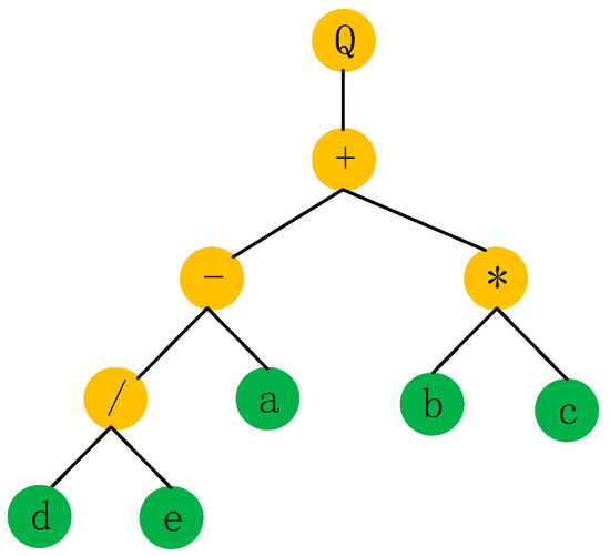
Figure 1.
The expression tree of chromosome Equation (1).
Based on the expression tree (Figure 1), the algebraic expression of Equation (1) can be determined:
With respect to GEP chromosomes, they have two merits: First, a GEP chromosome can be easily decoded, and the process is quite simple. Second, a GEP chromosome has a constant length, but the effective chromosome length may be less than or equal to the GEP chromosome length; this characteristic is convenient for further operation in the GEP algorithm [22,23].
The chromosomes are composed of two parts: a head and a tail. The head of a chromosome can contain many functional symbols and terminal symbols; however, the tail of a GEP chromosome can only consist of terminal symbols. The head length is determined according to specific circumstances, and the tail length is determined by Equation (3) [29,30]:
where t is the tail length, h is the head length, and n is the head maximum argument.
In this work, the GEP was utilized to implement the combination of creep bodies (elastic bodies, viscous bodies, plastic bodies, or other user-defined creep bodies). To implement the combination of creep units, the function symbols are connected in series (‘+’) and parallel connections (‘||’), whereas the terminal symbols are the creep bodies, such as elastic bodies, viscous bodies, and plastic bodies. Subsequently, a creep model can be represented by a GEP chromosome:
where ‘+’ represents the connection in the series, ‘||’ represents the parallel connection, ‘H’ represents the elastic body, ‘Y’ represents the plastic body, and ‘N’ represents the viscous body. Then, the GEP chromosome (Equation (4)) can be decoded into an expression tree (Figure 2) [31].
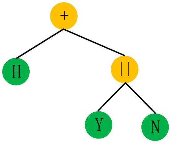
Figure 2.
Creep model expression tree.
Moreover, the corresponding creep model can be obtained from Figure 2, which is shown below (Figure 3).
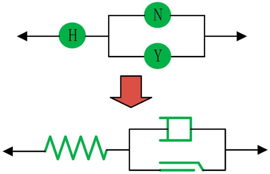
Figure 3.
Creep model (Bingham creep model).
Based on the analysis above, it can be concluded that a creep GEP chromosome can be easily transformed into a creep model. In accordance with the decoded creep model, the constitutive equation can be derived based on the creep model:
By combining the creep experimental data and Equation (5), the fitness of the creep model can be determined. In this paper, the fitness coefficient is used to define the fitness of the creep model, which can be calculated according to Equation (6) [32].
where is the measured strain from the experiments, is the average strain from the physical experiments, is the predicted strain based on the constitutive equation, and n is the total number of experimental datasets. Notably, the excellent prediction index for an empirical formula is 1 for R2 in theory.
To obtain a creep model based on the GEP algorithm, the following procedure was used:
- (1)
- The basic parameters of the GEP algorithm are initialized, and the experimental data are prepared; moreover, the experimental conditions are determined.
- (2)
- Creep model chromosomes are generated (the creep model chromosomes are generated for the first time), and the creep model chromosomes are decoded into the creep constitutive model.
- (3)
- Based on the creep constitutive model, the corresponding constitutive equations are deduced. Combining the experimental data, experimental conditions, and constitutive equations, the fitness of every individual creep chromosome is calculated via Equation (6).
- (4)
- Based on the calculation results, if the calculation result meets the termination condition, the calculation is finished, or the process continues to the next step.
- (5)
- Certain creep model chromosomes with high fitness values are selected, whereas the creep chromosomes with low fitness values are deleted, which obeys the rule of the fittest of survival.
- (6)
- When the gene in the chromosome is mutated, in the mutation process, the function symbols and terminal symbols in the head of the chromosome can be mutated into terminal symbols or function symbols; however, the terminals can only be mutated into terminal symbols in the tail of the chromosome.
- (7)
- The transposition and recombination of chromosomes are the same as those in the genetic algorithm. Go to step 2.
- (8)
- For convenience in implementing the GEP to establish the creep model, the flow chart is given in Figure 4.
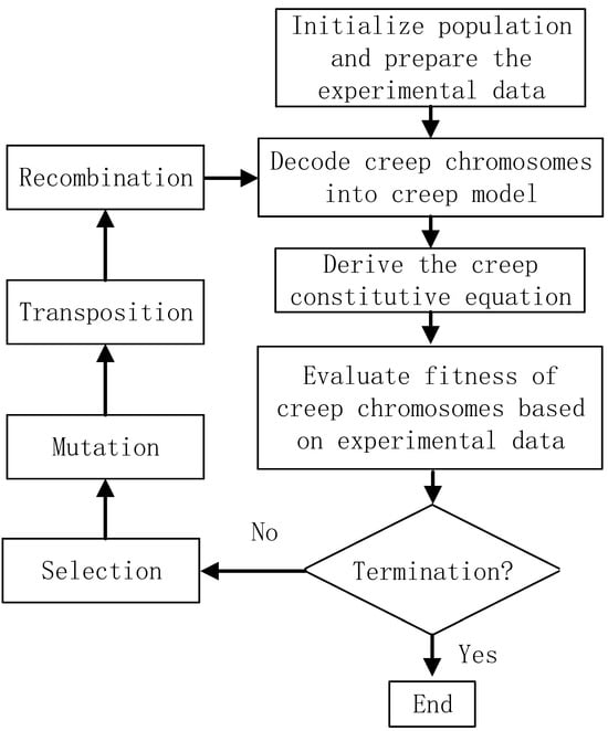 Figure 4. A flow chart of the process of establishing a creep model via gene expression programming.
As shown in Figure 4, the idea of GEP is based on the Darwinian concept of the survival and reproduction of the fittest, and the genetic operators in the GEP algorithm are composed of four procedures: selection, mutation, transposition, and recombination. For selection, the chromosomes are selected according to the corresponding fitness value and the roulette wheel sampling method [30]. Notably, any symbols in the head can be replaced by other symbols in the mutation process, whereas the symbols in the tail can be replaced only by terminal symbols. In addition, the mutation rate should be within a certain range (from 0.01 to 0.1) [33,34,35,36]. With respect to transposition, the gene in the GEP chromosome can be moved to other locations, and the transposition rate should be within the range of 0.010.1 [22,23]. The recombination process of the GEP algorithm is the same as that of the genetic algorithm [24].
2.2. Improved Gene Expression Programming
In practice, the convergence rate of the GEP is slow, and the number of iterations is too high when the termination criterion is satisfied. Adler [37] reported that modifying the mutation range rate based on the simulated annealing algorithm [38,39] can accelerate convergence. However, the GEP algorithm contains a mutation process, and the improvement can be used with the GEP algorithm as well. Based on Adler’s study, the fitness of chromosomes in the roulette wheel sampling procedure [40] can be changed as follows:
where is the fitness of the th chromosome, is the fitness of the th chromosome in roulette wheel sampling [40], is the size of the population, and is the temperature. The temperature is changed according to the evolution time (Equation (8)).
where is the initial temperature, is the present evolution time, and is the temperature after evolution times.
In Adler’s study, mutation occurred based on the simulated annealing algorithm. When the fitness of the chromosome after mutation is greater than before, mutation will occur without a doubt, or mutation will occur at a probability of . is the fitness of the th chromosome before mutation, and is the fitness of the th chromosome after mutation.
Furthermore, changing the recombination probability of individuals can accelerate the convergence rate. Yu et al. [41] proposed an algorithm to change the recombination rate according to the specific situation:
where is the recombination probability of the th individual; is the maximum evolution time; is the present evolution time; is 0.6; is the fitness of the th individual; is the maximum fitness of the population for the present evolution; and is the mean fitness of the population for the present evolution. By adopting these techniques, individuals with low fitness should involve recombination more frequently, which is helpful for producing good generations with high fitness. The individuals with high fitness values should be preserved, and the corresponding recombination probability should be lower.
For convenience in implementing improved GEP, the flow chart of improved GEP is illustrated in Figure 5.
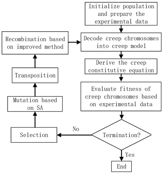
Figure 5.
A flow chart of improved gene expression programming.
To obtain a creep model based on the experimental data via the improved GEP algorithm, the corresponding program was complied with via the Python language.
2.3. Validation of Determining Creep Models Based on Improved Gene Expression Programming
To verify the validity of determining a creep model via improved gene expression programming, two examples are given below.
2.3.1. The Construction of the Creep Model of Siltstone
In the first example, the siltstone from the Niumasi Shuitou Coal Mine in the Hunan province of China was taken as an example to illustrate how to obtain a creep model based on the improved gene expression programming. The basic parameters of the siltstone are listed in Table 1.

Table 1.
Basic mechanical parameters of the siltstone.
In our experiments, the sample was under the uniaxial compressive loading state, and four stress levels were utilized: 21 MPa, 26 MPa, 31 MPa, and 36 MPa. The time for every stress level was 20 h; after 20 h, the stress was loaded to the next stress level at a speed of 1 MPa/s. The strain–time experimental data, which are displayed in Figure 6, were subsequently obtained.
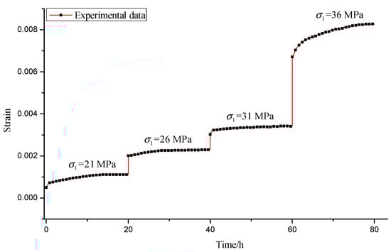
Figure 6.
Creep experimental data of siltstone under uniaxial compression.
For convenience in obtaining the creep model of the siltstone, the experimental data were divided into four parts when the stress levels were 21 MPa, 26 MPa, 31 MPa, and 36 MPa, as shown in Figure 7.
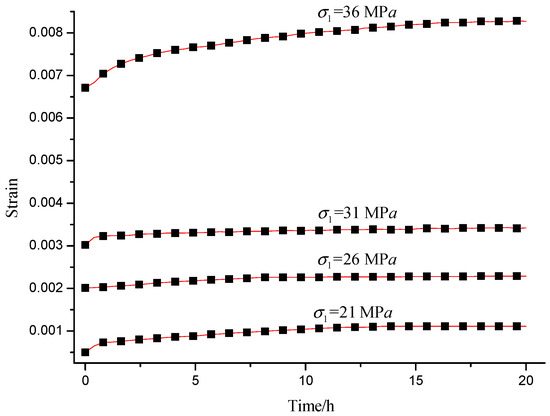
Figure 7.
Experimental data of the creep experiments when the stress level is 21 MPa, 26 MPa, 31 MPa, and 36 MPa.
In this example, the function set is (N: viscous creep body, Y: plastic creep body, H: elastic creep body), and the function set is (+: connection in series and ||: parallel connections), the head of a chromosome is 15, and the maximum argument of all functions in head is 30. Based on Equation (3), the tail length of a chromosome is 436.
Based on the improved gene expression programming, the creep constitutive model was obtained, and an improved GEP chromosome was obtained:
The expression tree can be expressed as follows (Figure 8):
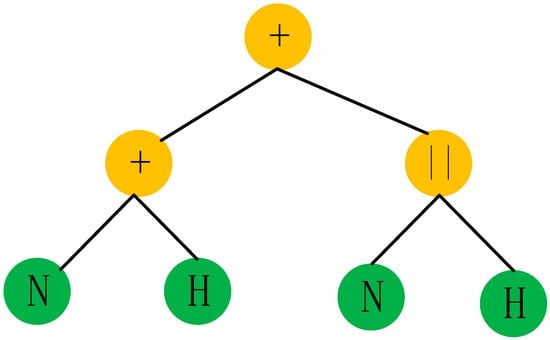
Figure 8.
The expression tree based on the chromosome code Equation (11).
From the analysis of Figure 8, it should be noted that the yield creep body (Y) did not appear, which means that the yield creep body was eliminated in the procedure of the improved GEP. The expression tree (Figure 8) can be decoded as a creep constitutive model, which is illustrated as follows (Figure 9).
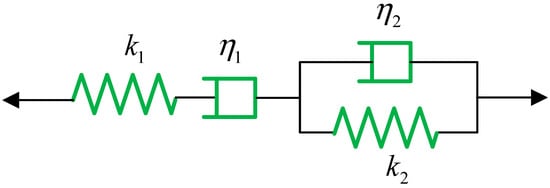
Figure 9.
Creep model obtained via improved GEP (Burgers model).
The corresponding constitutive equation was as follows.
Table 2.
The parameters of the creep body in the creep model.
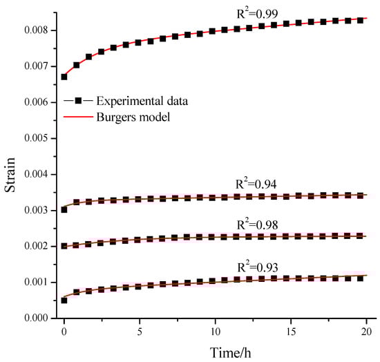
Figure 10.
The fitting result.
An analysis of the data in Table 2 and Figure 10 reveals that the theoretical curves of the creep model obtained via improved gene expression programming are in good agreement with the experimental data, with a correlation coefficient () above 0.93. The validity of the improved GEP for establishing the creep model was verified.
2.3.2. The Establishment of the Creep Model of Mine Rock
Moreover, an extra creep body can be added to the proposed method. For example, Chen et al. [42] proposed a creep yield joint (CYJ) body; based on the definition of the CYJ creep body, its constitutive model can be described as follows:
The creep characteristics of the CYJ creep body were determined by three parameters: the fitting parameter , the viscosity parameter , and the strain parameter .
Equation (13) can be written as follows:
where .
To further verify the validity of the proposed method, another example was provided. Zhang et al. [10] studied the creep behaviour of the rock from the Jingchuang mine. Loading and unloading creep experiments under uniaxial compression were conducted. The uniaxial compressive strength of the rock is 44.5 MPa. The stress level contains five levels, namely, 8.089 MPa, 12.782 MPa, 17.473 MPa, 23.565 MPa, and 33.807 MPa, and the loading time determines the strain variation. When the axial strain variation is less than 0.001 mm/h, the strain tends to stabilize, and then the stress is unloaded to 0 MPa for 24 h; then, the next stress level begins. In the experiments, the loading and unloading speed was 0.5 MPa/s. based on the experiments. The strain–time curve was obtained, which is illustrated in Figure 11.
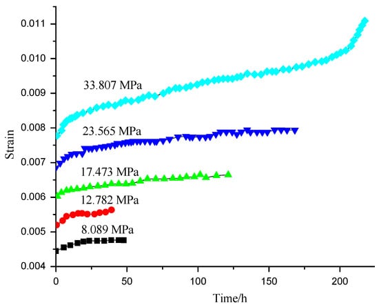
Figure 11.
Strain–time curves from the creep experiments [10].
In this example, the CYJ model was added to the function set: (N: viscous creep body, Y: plastic creep body, H: elastic creep body, and : CYJ creep body).
By using the improved gene expression programming method, the creep chromosome model was obtained:
Then, Equation (15) can be decoded as a tree (Figure 12):
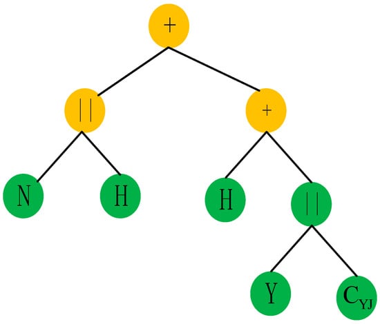
Figure 12.
Creep model tree of mine rock.
The subsequent creep model is illustrated in Figure 13.
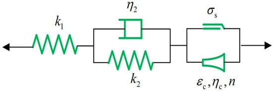
Figure 13.
The obtained creep model.
The constitutive equation for the creep model (Figure 13) can be expressed as follows:
The fitting results are shown in Figure 13, and the basic parameters of the creep model are listed in Table 3.
Table 3.
Fitting parameters of the obtained creep model.
From the analysis of Table 3 and Figure 14, it can be concluded that improved gene expression programming can be applied to establish a creep model by using creep bodies. The creep model is in good agreement with the experimental data, with the above correlation coefficient above 0.91. The results indicate that the proposed technique is reliable and can be applied in practice.
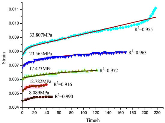
Figure 14.
The fitting results.
3. Discussion
Creep behaviour is one of the most important mechanical behaviours of rocks, and studies on the creep characteristics of rocks are meaningful. In this paper, studies related to the creep behaviour of rocks are reviewed. Based on techniques for describing the creep behaviour of rock materials, two types of creep models of rock materials are generally classified: theoretical formulas and combinations of creep bodies. From the analysis of these two methods, researchers have attempted to describe the creep characteristics of rock materials more comprehensively and more accurately, and an increasing number of creep models have been proposed. Moreover, combinations of creep bodies are commonly used to describe the creep behaviour of rock materials. By using the three traditional creep bodies, the primary creep stage and secondary creep stage can be depicted; however, the tertiary creep stage cannot be fully repeated. To overcome this problem, different kinds of new creep bodies have been invented, which have promoted the development of rock creep mechanics.
However, the procedure of creep models established by using creep bodies can generally be divided into two steps: first, the experimental data are tidied; second, the creep bodies are selected, and the characteristics of the experimental data are combined. For the establishment of a creep model by combining creep bodies, the process of determining a creep model is obviously quite subjective: the construction of a creep model is determined by the researchers’ experience, which is not scientific enough.
To avoid the subjectivity of establishing a creep mode by using creep bodies, in this paper, the gene expression programming algorithm was utilized; by manufacturing the creep model chromosome and the creep model chromosome population involved, the best creep model can be determined. To accelerate the convergence rate of the calculation, the gene expression programme was further improved, and the corresponding Python programme was used to implement improved gene expression programming. To verify the validity of the improved gene expression programme, two examples were provided based on the creep test data under loading. The fitness of the established creep model to the experimental data is quite satisfactory, indicating the fidelity of the proposed method.
However, it should be noted that the obtained creep model was based on the creep bodies in the terminal set, and more creep bodies should be added. Moreover, in this paper, the proposed method was only used for the combination of creep bodies, and the combination of creep bodies and theoretical formulas was not implemented, which is our next task.
4. Conclusions
In this paper, studies on creep models of rock were reviewed, and improved gene expression programming was used to obtain a creep model. The prominent work of this paper can be summarized as follows:
- (1)
- A study on the creep model for describing the creep behaviour of rocks was reviewed, and the types of creep models of rock can generally be classified into two categories: theoretical formulas and combinations of creep bodies.
- (2)
- To avoid the subjectivity of establishing the creep model, in this paper, a technique using improved gene expression programming to obtain the creep model was proposed. Two examples were provided to verify the validity of the proposed technique. By combining the experimental data and improved gene expression programming, creep models for siltstone and mine rock were developed, and the fitting results indicated that improved gene expression programming can be applied to establish creep models for rock.
Author Contributions
Software, J.C. (Junwen Chen); Validation, S.G.; Formal analysis, C.Q. and J.H.; Writing—original draft, P.F.; Writing—review & editing, M.W.; Funding acquisition, J.C. (Junhua Chen). All authors have read and agreed to the published version of the manuscript.
Funding
This study were funded by the science and technology programme of the geological bureau of Hunan province (2024013), supported by the Department of Natural Resources of Hunan Province, China (2024-08) and the Hunan Provincial Natural Science Foundation of China (2025JJ80001). All authors have read and agreed to the published version of the manuscript.
Institutional Review Board Statement
Not applicable.
Informed Consent Statement
Not applicable.
Data Availability Statement
The original contributions presented in this study are included in the article. Further inquiries can be directed to the corresponding author.
Conflicts of Interest
The authors declare that they have no conflicts of interest.
References
- Tan, T.K.; Kang, W. On the locked in stress, creep and dilatation of rocks and the constitutive equations. Chin. J. Rock Mech. Eng. 1991, 10, 299–312. [Google Scholar]
- Shao, J.F.; Zhu, Q.Z.; Su, K. Modeling of creep in rock materials in terms of material degradation. Comput. Geotech. 2003, 30, 549–555. [Google Scholar] [CrossRef]
- Jia, Y.; Song, X.C.; Duveau, G.; Su, K.; Shao, J.F. Elastoplastic damage modelling of argillite in partially saturated condition and application. Phys. Chem. Earth. 2007, 32, 656–666. [Google Scholar] [CrossRef]
- Bourgeois, F.; Shao, J.F.; Ozanam, O. An elastoplastic model for unsaturated rocks and concrete. Mech. Res. Commun. 2002, 29, 383–390. [Google Scholar] [CrossRef]
- Malan, D.F. Time-dependent behaviour of deep level tabular excavations. Rock Mech. Rock Eng. 1999, 32, 123–155. [Google Scholar] [CrossRef]
- Miura, K.; Okui, Y.; Horii, H. Micromechanics-based prediction of creep failure of hard rock for long-term safety of high-level radioactive waste disposal system. Mech. Mater. 2003, 35, 587–601. [Google Scholar] [CrossRef]
- Korzeniowski, W. Rheological Model of Hard Rock Pillar. Rock Mech. Rock Eng. 1991, 24, 155–166. [Google Scholar] [CrossRef]
- Boukharov, G.N.; Chanda, M.W.; Boukharov, N.G. The three processes of brittle cystalline rock creep. Int. J. Rock Mech. Min. 1995, 32, 325–335. [Google Scholar] [CrossRef]
- Zhang, S.G.; Liu, W.B.; Lv, H.M. Creep energy damage model of rock graded loading. Results Phys. 2019, 12, 1119–1125. [Google Scholar] [CrossRef]
- Zhang, Y.P.; Cao, P.; Zhao, Y.L. Visco-plastic rheological properties and a nonlinear creep model of soft rocks. J. China Univ. Min. Technol. 2009, 38, 34–40. [Google Scholar]
- Wu, L.Z.; Luo, X.H.; Li, S.H. A new model of shear creep and its experimental verification. Mech. Time-Depend Mater. 2020, 25, 429–446. [Google Scholar] [CrossRef]
- Zhang, L.Y.; Yang, S.Y. Unloading rheological test and model research of hard rock under complex conditions. Adv. Mater. Sci. Eng. 2020, 2020, 3576181. [Google Scholar] [CrossRef]
- Wang, Y.C.; Wang, Y.Y. Study on nonlinear viscoelastoc-plastic creep model of deep soft rock. Adv. Mater. Res. 2012, 430–432, 168–172. [Google Scholar]
- Wang, X.G.; Huang, L.; Zhang, J.R. A rheological model of sandstones considering response to thermal treatment. Adv. Civ. Eng. 2019, 2019, 2143748. [Google Scholar] [CrossRef]
- Chen, L.; Wang, C.P.; Liu, J.F.; Liu, Y.M.; Liu, J.; Su, R.; Wang, J. A damage-mechanism-based creep model considering temperature effect in granite. Mech. Res. Commun. 2014, 56, 76–82. [Google Scholar] [CrossRef]
- He, Z.L.; Zhu, Z.D.; Wu, N.; Wang, Z.; Cheng, S. Study on time-dependent behaviour of granite and the creep model based on fractional derivative approach considering temperature. Math. Probl. Eng. 2016, 2016, 8572040. [Google Scholar] [CrossRef]
- Liu, L.; Wang, G.M.; Chen, J.H.; Yang, S. Creep experiment and rheological model of deep saturated rock. Trans. Nonferr. Met. Soc. 2013, 23, 478–483. [Google Scholar] [CrossRef]
- Wang, J.G.; Sun, Q.L.; Liang, B.; Yang, P.J.; Yu, Q.R. Mudstone creep experiment and nonlinear damage model study under cyclic disturbance load. Sci. Rep. 2020, 10, 9305. [Google Scholar] [CrossRef]
- Lv, S.R.; Wang, W.Q.; Liu, H.Y. A creep damage constitutive model for a rock mass with nonpersistent joint under uniaxial compression. Math. Probl. Eng. 2019, 2019, 4361458. [Google Scholar] [CrossRef]
- Wu, F.; Gao, R.B.; Zou, Q.L.; Chen, J.; Liu, W.; Peng, K. Long-term strength determination and nonlinear creep damage constitutive model of salt rock based on multistage creep tests: Implications for underground natural gas storage in salt cavern. Energy Sci. Eng. 2020, 8, 1592–1603. [Google Scholar] [CrossRef]
- Han, Y.; Ma, H.L.; Yang, C.H.; Zhang, N.; Daemen, J.J.K. A modified creep model for cyclic characterization of rock salt considering the effects of the mean stress, half-amplitude and cycle period. Rock Mech. Rock Eng. 2020, 53, 3223–3236. [Google Scholar] [CrossRef]
- Ferreira, C. Gene expression programming: A new adaptive algorithm for solving problems. Complex. Systems 2001, 13, 87–129. [Google Scholar]
- Ferreira, C. Gene expression programming in problem solving. In Soft Computing and Industry-Recent Applications; Roy, R., Koppen, M., Ovaska, S., Furuhashi, T., Hoffmann, F., Eds.; Springer: Berlin/Heidelberg, Germany, 2002; pp. 635–654. [Google Scholar]
- Faradonbeh, R.S.; Armaghani, D.J.; Monjezi, M.; Mohamad, E.T. Genetic programming and gen expression programming for flyrock assessment due to mine blasting. Int. J. Rock Mech. Min. 2016, 88, 254–264. [Google Scholar] [CrossRef]
- Steeb, W.H. The Nonlinear Workbook: Chaos, Fractals, Cellular Automata, Neural Networks, Genetic Algorithms, Gene Expression Programming, Support Vector Machine, Wavelets, Hidden Markov Models, Fuzzy Logic with C++, Java and Symbolic C++ Programs, 3rd ed.; World Scientific: Singapore, 2011. [Google Scholar]
- Brownlee, J. Clever Algorithms: Nature-Inspired Programming Recipes; Lulu: Morrisville, NC, USA, 2011. [Google Scholar]
- Karakus, M. Function identification for the intrinsic strength and elastic properties of granitic rock via genetic programming (GP). Comput. Geosci. 2011, 37, 1318–1323. [Google Scholar] [CrossRef]
- Koza, J.R. Genetic Programming: On the Programming of Computers by Means of Natural Selection; MIT Press: Cambridge, MA, USA, 1992. [Google Scholar]
- Baykasoglu, A.; Gullu, H.; Canakci, H.; Ozbakir, L. Prediction of compressive and tensile strength of limestone via genetic programming. Expert Syst. Appl. 2008, 35, 111–123. [Google Scholar] [CrossRef]
- Silva, S.; Almeida, J. Dynamic maximum tree depth—A simple technique for avoiding bloat in tree-based GP. In Genetic and Evolutionary Computation—GECCO 2003: Genetic and Evolutionary Computation Conference Chicago, IL, USA, 12–16 July 2003 Proceedings, Part II; Cantu-Paz, E., Foster, J.A., Deb, K., Eds.; Springer: Berlin/Heidelberg, Germany, 2003; pp. 1776–1787. [Google Scholar]
- Liu, K.Y.; Xue, Y.T.; Zhou, H. Study on 3D nonlinear visco-elastic-plastic creep constitutive model with parameter unsteady of soft rock based on improved Bingham model. Rock Soil Mech. 2018, 39, 4157–4164. [Google Scholar]
- Nakagawa, S.; Johnson, P.C.D.; Schielzeth, H. The coefficient of determination R-2 and intra-class correlation coefficient from generalized linear mixed-effects models revisited and expanded. J. R. Soc. Interface 2017, 14, 20170213. [Google Scholar] [CrossRef] [PubMed]
- Teodorescu, L.; Sherwood, D. High energy physics event selection with gene expression programming. Comput. Phys. Commun. 2008, 178, 409–419. [Google Scholar] [CrossRef]
- Yang, Y.; Li, X.; Gao, L.; Shao, X. A new approach for predicting and collaborative evaluating the cutting force in face milling based on gene expression programming. J. Netw. Comput. Appl. 2013, 36, 1540–1550. [Google Scholar] [CrossRef]
- Kayadelen, C. Soil liquefaction modeling by genetic expression programming and neuro-fuzzy. Expert Syst. Appl. 2011, 38, 4080–4087. [Google Scholar] [CrossRef]
- Mollahasani, A.; Alavi, A.H.; Gandomi, A.H. Empirical modeling of plate load test moduli of soil via gene expression programming. Comput. Geotech. 2011, 38, 281–286. [Google Scholar] [CrossRef]
- Adler, D. Genetic algorithms and simulated annealing: A marriage proposal. In Proceedings of the IEEE International Conference on Neural Networks, San Francisco, CA, USA, 28 March–1 April 1993; pp. 1104–1109. [Google Scholar]
- Dupanloup, I.; Schneider, S.; Excoffier, L. A simulated annealing approach to define the genetic structure of populations. Mol. Ecol. 2002, 11, 2571–2581. [Google Scholar] [CrossRef] [PubMed]
- Kipkpatrick, S.; Gelatt, C.D.; Vecchi, M.P. Optimization by simulated annealing. Science 1983, 220, 671–680. [Google Scholar] [CrossRef] [PubMed]
- Weng, M.C.; Tsai, L.S.; Hsieh, Y.M.; Jeng, F.S. An associated elastic-viscoplastic constitutive model for sandstone involving shear-induced volumetric deformation. Int. J. Rock Mech. Min. 2010, 47, 1263–1273. [Google Scholar] [CrossRef]
- Yu, Y.Y.; Chen, Y.; Li, T.Y. Improved genetic algorithm for solving TSP. Control. Decis. 2014, 29, 1483–1488. [Google Scholar]
- Chen, Y.J.; Pan, C.L.; Cao, P.; Wang, W.X. A new mechanical model for soft rock rheology. Rock Soil Mech. 2003, 24, 209–214. [Google Scholar]
Disclaimer/Publisher’s Note: The statements, opinions and data contained in all publications are solely those of the individual author(s) and contributor(s) and not of MDPI and/or the editor(s). MDPI and/or the editor(s) disclaim responsibility for any injury to people or property resulting from any ideas, methods, instructions or products referred to in the content. |
© 2025 by the authors. Licensee MDPI, Basel, Switzerland. This article is an open access article distributed under the terms and conditions of the Creative Commons Attribution (CC BY) license (https://creativecommons.org/licenses/by/4.0/).