Article

A Lightweight Neural Network for Denoising Wrapped-Phase Images Generated with Full-Field Optical Interferometry

by
Muhammad Awais
1,
Younggue Kim
1,
Taeil Yoon
2,
Wonshik Choi
2 and
Byeongha Lee
1,*
1
Department of Electrical Engineering and Computer Science, Gwangju Institute of Science and Technology, Gwangju 61005, Republic of Korea
2
Department of Physics, Korea University, Seoul 02855, Republic of Korea
*
Author to whom correspondence should be addressed.
Appl. Sci. 2025, 15(10), 5514; https://doi.org/10.3390/app15105514
Submission received: 9 April 2025 / Revised: 7 May 2025 / Accepted: 12 May 2025 / Published: 14 May 2025
(This article belongs to the Special Issue Computer-Vision-Based Biomedical Image Processing)

Abstract

Phase wrapping is a common phenomenon in optical full-field imaging or measurement systems. It arises from large phase retardations and results in wrapped-phase maps that contain essential information about surface roughness and topology. However, these maps are often degraded by noise, such as speckle and Gaussian, which reduces the measurement accuracy and complicates phase reconstruction. Denoising such data is a fundamental problem in computer vision and plays a critical role in biomedical imaging modalities like Full-Field Optical Interferometry. In this paper, we propose WPD-Net (Wrapped-Phase Denoising Network), a lightweight deep learning-based neural network specifically designed to restore phase images corrupted by high noise levels. The network architecture integrates a shallow feature extraction module, a series of Residual Dense Attention Blocks (RDABs), and a dense feature fusion module. The RDABs incorporate attention mechanisms that help the network focus on critical features and suppress irrelevant noise, especially in high-frequency or complex regions. Additionally, WPD-Net employs a growth-rate-based feature expansion strategy to enhance multi-scale feature representation and improve phase continuity. We evaluate the model’s performance on both synthetic and experimentally acquired datasets and compare it with other state-of-the-art deep learning-based denoising methods. The results demonstrate that WPD-Net achieves superior noise suppression while preserving fine structural details even with mixed speckle and Gaussian noises. The proposed method is expected to enable fast image processing, allowing unwrapped biomedical images to be retrieved in real time.

1. Introduction

Interferometry is a highly precise optical technique widely used for imaging or analyzing shape, deformation, or refractive index distribution [1]. A common phenomenon in interferometric systems is phase wrapping, which occurs when the measured phase exceeds the principal range of −π to π, resulting in wrapped-phase images or maps. These wrapped-phase images contain essential information about the object’s surface characteristics, but a phase unwrapping process is required to reconstruct the true phase distribution [2]. However, noise, particularly speckle and Gaussian noise, can complicate the unwrapping process and reduce overall accuracy [3,4].
Speckle noise arises from the rough surface of the object under imaging and is highly non-stationary. It causes localized variations in intensity and phase, making it difficult to remove with conventional filtering and often leading to unwrapping errors [5,6]. On the other hand, Gaussian noise introduces random fluctuations across both smooth and detailed regions, reducing the signal-to-noise ratio (SNR) [7,8]. The combined presence of these noise types significantly impacts the quality of wrapped-phase maps, especially when simple algorithms are used for unwrapping. Therefore, an effective denoising process before phase unwrapping is crucial, as it can remove noise artifacts while preserving structural details, ensuring more reliable phase reconstruction.
Traditional denoising approaches such as sine/cosine filters [3,4] and windowed Fourier transforms [9,10] have been used in wrapped-phase denoising, but these methods often involve high computational costs and require extensive parameter tuning, limiting their adaptability in practical applications. With the emergence of deep learning, denoising techniques have advanced significantly. Convolutional Neural Networks (CNNs) [11] and their variants have been successfully applied in optical domains such as synthetic aperture radar (SAR) imaging [12], multiscale decomposition [13], hyperspectral imaging [14], and optical coherence tomography (OCT) [15,16]. These approaches have shown promising results in wrapped-phase denoising tasks as well [17]. For instance, the Denoising Convolutional Neural Network (DnCNN) [18] was introduced to remove Gaussian noise through supervised learning with paired training data. However, it is less effective against non-Gaussian noise such as speckle noise.
To address the problems of speckle noise, various CNN-based networks have been developed. The fringe pattern denoising CNN (FPD-CNN) [19] was proposed for digital speckle pattern interferometry, while V-Net [20] facilitated fringe denoising and normalization. Montresor et al. [21] trained a CNN on real speckle-corrupted holograms, significantly improving denoising performance in digital holographic vibrometry. Fang et al. [22] employed a conditional generative adversarial network (cGAN) to achieve high-quality speckle reduction, enhancing phase measurement accuracy. Yan et al. [23] introduced a method for denoising wrapped-phase images, aimed at improving defect detection in structural diagnostics.
Several hybrid models have also been explored. A convolutional and Fourier neural network architecture combining CNNs with Fourier neural operators was proposed to extract spatial and frequency features simultaneously [24]. Zhang et al. [25] proposed a speckle denoising convolutional neural network (SDCNN) aimed at suppressing speckle noise in digital speckle shearography, preserving texture through optimized loss functions.
Li et al. [26] introduced a dilated-blocks-based deep convolution neural network (DBDNet) designed for high-speckle environments. Its extended version [27] employed a combined MS-SSIM and L1 loss to enhance denoising accuracy. Wang et al. [28] presented an attention-driven denoising approach to address fringe patterns with variable density. He et al. [29] proposed the local-global channel transformer network (LGCT-Net), which integrates transformers [30] with CNNs to improve the performance of discontinuous and diverse phase patterns. Yu et al. [31] proposed a phase denoising network (PDNet) for InSAR phase denoising, which learns non-local self-similarity from diverse wrapped-phase images and filters noise without relying on kernel-based averaging, thereby preserving resolution and phase integrity.
For batch denoising of images obtained through electronic speckle pattern interferometry (ESPI), Hao et al. [32] and Xu et al. [33] proposed different approaches. Hao’s CNN-based framework processed multiple noisy images in parallel, while Xu’s multi-dilated dense network (MDD-Net) focused on preserving structural integrity. Similarly, Gurrola et al. [34] implemented a U-Net-based model and Yan et al. [35] introduced a deep CNN (DCNN) for generalized fringe pattern denoising.
Despite recent progress, several challenges still remain in wrapped-phase image denoising. Most existing methods are designed to handle either Gaussian or speckle noise individually but often fail when both types are present. This difficulty arises from the fundamental differences between the two: Gaussian noise is additive and statistically uniform, while speckle noise is multiplicative and highly variable. These differences require distinct strategies for effective removal, making it hard for a single model to perform well across both noise types. In addition, many current techniques demand significant computational resources and manual parameter tuning, making them less suitable for real-time applications. Their dependence on customized training datasets also limits adaptability and scalability. These limitations highlight the need for a more efficient and general approach that can handle diverse noise conditions with accuracy and consistency.
To address the challenges in wrapped-phase denoising, we introduce WPD-Net (Wrapped-Phase Denoising Network), a robust and lightweight deep learning model designed to effectively handle both Gaussian and speckle noises. The network features a carefully structured architecture that begins with multiple convolutional layers for initial feature extraction, followed by residual dense attention blocks (RDABs). These RDABs extend conventional residual dense blocks by incorporating attention mechanisms, allowing the network to focus more effectively on relevant noisy regions and improve feature propagation. A dense feature fusion (DFF) module further combines hierarchical features to refine details and preserve the structural integrity of wrapped-phase images. Together, these components enable WPD-Net to capture complex noise patterns and restore clean high-quality phase images, while maintaining fast and accurate denoising performance without the need for large-scale training datasets.
The main contributions of this study are as follows:
  • A synthetic dataset is generated by combining a ramp function and multiple Gaussian functions, incorporating various degrees of randomness and noise levels to enhance the model’s capability to handle diverse noise conditions.
  • We propose WPD-Net, specifically designed to extract phase information distorted by noise while preserving fine structural details. The architecture includes RDABs that enhance phase reconstruction.
  • Instead of using only the mean squared error (MSE) loss, we employ a dynamic hybrid loss function that adaptively balances Structural Similarity Index (SSIM) and MSE during training for optimal intensity and structural preservation.
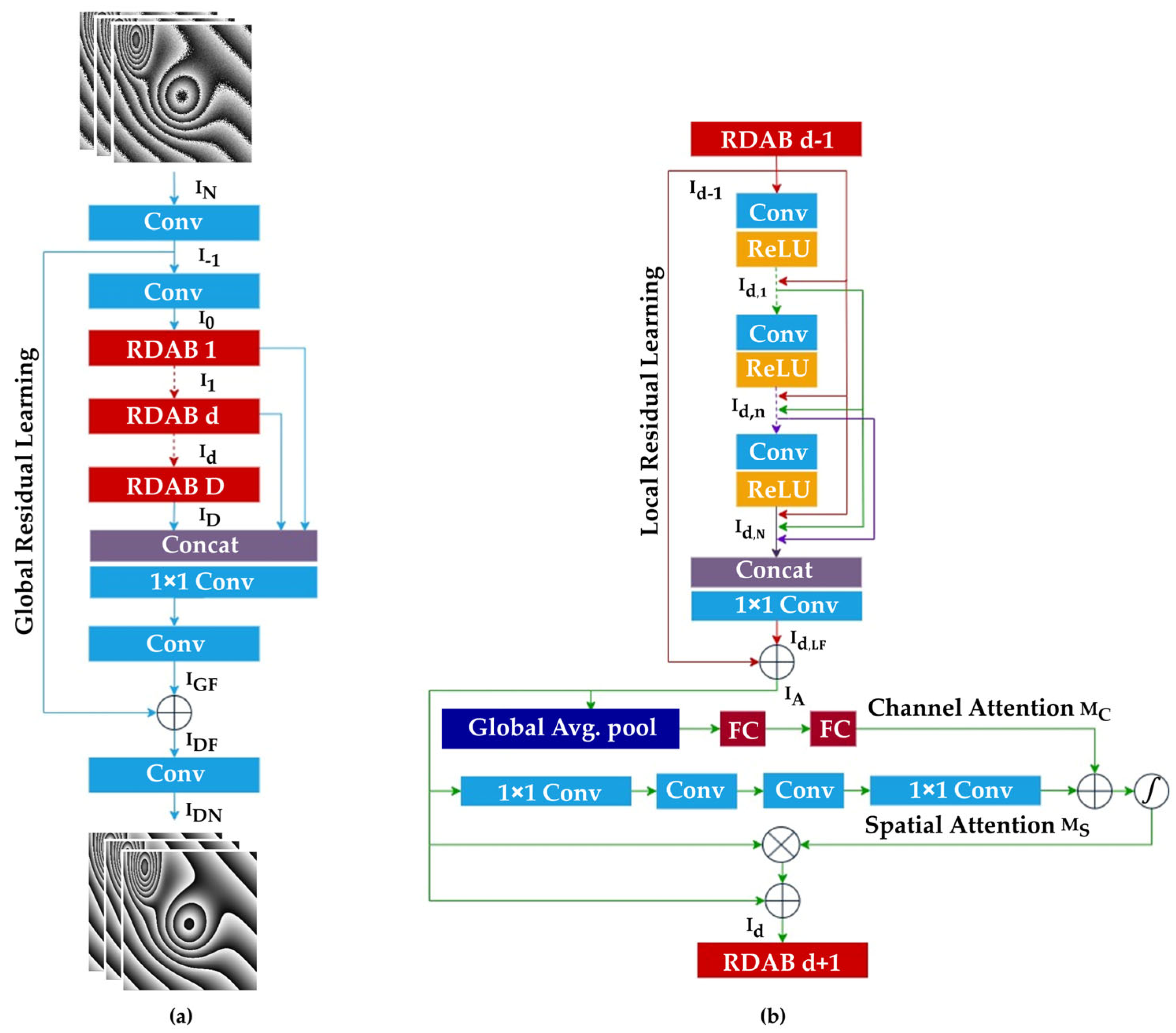
To evaluate the performance of the proposed WPD-Net, we conduct experiments on both synthetic data and real data acquired from a custom-built full-field digital holographic interferometry setup. For quantitative assessment, we use three evaluation metrics: MSE, peak signal-to-noise ratio (PSNR), and SSIM. Comparisons are also made with other deep learning-based methods. Furthermore, ablation studies are conducted to analyze the impact of different loss functions and architectural components.

2. Method

The proposed WPD-Net, illustrated in Figure 1a, is designed to effectively remove noise while preserving structural details in wrapped-phase images. The network consists of three main stages: a shallow feature extraction (SFE) module, residual dense attention blocks (RDABs), and a dense feature fusion (DFF) module. These components work together to capture both local and global features. The input to the network is a noisy wrapped-phase image of size 256 × 256 pixels, and the output is a denoised image of the same resolution.
The input noisy wrapped-phase image, denoted as I N , is first processed through the SFE module, consisting of two convolutional layers. This stage enhances primary structural features while reducing noise. The shallow feature extraction is defined as:
I 1 = H SFE 1 I N ,
I 0 = H SFE 2 I 1 .
where HSFE1 and HSFE2 represent convolution operations in the SFE module. The feature map I 1 is the output of the first convolutional layer in the SFE module. The feature map I 0 , output from the SFE module, serves as the input to the following RDAB. Each RDAB consists of multiple convolutional layers with ReLU activation [36], followed by attention mechanisms [37] to enhance feature attention in both spatial and channel dimensions. Given D RDABs, the output of the d-th RDAB, denoted by I d , is recursively computed as:
I d = H RDAB , d I d 1
where H RDAB , d denotes the function of the d-th RDAB.
After passing through all RDABs, the DFF module integrates features from all preceding layers. The feature map I DF produced by the DFF module is given by:
I DF = H DFF I 1 , I 0 , I 1 , ,   I D .
Finally, the denoised wrapped-phase image I DN is obtained as:
I DN = H F i n a l I DF .
Here, H F i n a l denotes the final convolution layer that maps the refined feature map I DF to the denoised wrapped-phase output I DN .

2.1. Residual Dense Attention Block (RDAB)

The RDABs, illustrated in Figure 1b, are designed to enhance feature extraction by combining densely connected convolutional layers, local feature fusion, local residual learning, and attention mechanisms. This architecture promotes information flow, encourages feature reuse, and improves noise suppression efficiency. A sequential memory mechanism is employed to propagate feature information between RDABs. This design maintains a continuous flow of learned features, facilitates effective gradient propagation, reduces the risk of vanishing gradients, and enhances the overall utilization of extracted information for noise removal.
Each RDAB adopts a growth-rate-based feature expansion strategy, which concatenates intermediate feature representations at different depths. The block comprises dilated convolutional layers with a 3 × 3 kernel, batch normalization (BN) [38], and ReLU activation functions to capture both fine and broad details. Additionally, spatial and channel attention mechanisms are incorporated at the end of each RDAB to guide the network’s focus toward informative spatial and channel features, particularly in regions heavily corrupted by noise. By combining outputs from different depths and emphasizing relevant features through attention, RDABs preserve both shallow and deep structural details crucial for accurate phase restoration.
Within each RDAB, let I d 1 and I d represent the input and output feature maps, respectively. The output of the n-th convolutional layer inside the RDAB is:
I d , n = σ W d , n [ I d 1 , I d , 1 , , I d , n 1 ]
where σ is the ReLU activation and W d , n represents the convolutional weights. Here, each convolution layer produces G new feature maps. To manage feature growth, local feature fusion is performed via a 1 × 1 convolution layer as:
I d , LF = H LFF [ I d 1 , I d , 1 , , I d , N ] .
Following fusion, local residual learning is performed by adding the fused output back to the input of the RDAB:
I A = I d 1 + I d , LF .
where I A denotes the intermediate output before attention enhancement.
To further enhance feature learning, each RDAB incorporates channel and spatial attention mechanisms that guide the network to focus on informative features and critical spatial regions. The intermediate feature map I A   R c × h × w , where c denotes the number of channels and h and w represent the spatial height and width, respectively, undergoes channel and spatial attention enhancement. First, channel attention is computed by compressing the spatial dimensions through global average pooling, producing a vector I C   R c × 1 × 1 . This vector is passed through two fully connected (FC) layers to capture inter-channel dependencies as:
M c I A = BN ( W 1 ReLU ( W 0 ( AvgPool I A ) + b 0 ) + b 1 ) .
where W 0 R ( c / r ) × c ,   b 0 R c / r ,   W 1 R c × ( c / r ) ,   b 1 R c , and r is the reduction ratio. BN denotes batch normalization.
Next, spatial attention is applied using a 1 × 1 convolution, followed by two 3 × 3 dilated convolutions to capture contextual information. A final 1 × 1 convolution and batch normalization are applied to generate the spatial attention map:
M s I A = BN ( f 3   1 × 1 ( f 2   3 × 3 ( f 1   3 × 3 ( f 0   1 × 1 ( I A ) ) ) ) ) .
Here, f i k × k denotes convolutional layers with specified filter sizes. The final attention map is computed by summing the channel and spatial attention maps, applying a sigmoid activation, and performing element-wise multiplication with the original input:
M I A = σ ( M c I A + M s I A )
To further interpret the role of attention mechanisms within WPD-Net, we visualize both spatial and channel attention maps with two noisy wrapped-phase images, generated from the first RDAB layer. Figure 2 illustrates the following: Figure 2(a-1,a-2) the input noisy wrapped-phase images; Figure 2(b-1,b-2) the spatial attention maps; Figure 2(c-1,c-2) the up-sampled visualizations of the channel attention vectors; and Figure 2(d-1,d-2) the combined attention maps formed by summing the spatial and the channel attention maps element-wise. The spatial attention maps retain the full spatial resolution (256 × 256), highlighting informative regions across the input image that are affected by strong noise or exhibit sharp phase transitions. In contrast, channel attention maps are inherently 1D vectors that assign weights to each feature channel without any spatial structure. We up-sample these 1D channel attention vectors to 2D visual maps of size 256 × 256 for better interpretation. This contributes to a deeper understanding of the role of attention mechanisms within RDABs.
The final RDAB output is:
I d = I A + I A     M I A .
Here, represents element-wise multiplication.

2.2. Dense Feature Fusion (DFF)

After extracting local features through RDABs, the DFF module globally fuses them as:
I GF =   H GFF [ I 1 , , I D ]
where the features are first concatenated and then fused through 1 × 1 and 3 × 3 convolutions. Global residual learning is then performed by combining the shallow feature map I 1 with the fused features as:
I DF   = I 1 + I GF
This residual connection ensures that early extracted features are preserved and reused, enhancing multi-scale learning. Finally, a convolutional layer produces the denoised output image.

2.3. Advantages of WPD-Net

The proposed WPD-Net offers several advantages over existing denoising networks. By employing RDABs, which integrate densely connected convolutional layers with both channel and spatial attention mechanisms, the network is able to effectively focus on informative regions while suppressing irrelevant noise. This design allows WPD-Net to preserve fine structural details and maintain phase continuity even under challenging noise conditions. The use of a growth-rate-based feature expansion strategy further enhances multi-scale feature extraction, enabling the network to capture both local and global phase variations. Additionally, the global residual learning mechanism in the DFF module strengthens feature propagation and helps retain important low-level features, leading to more accurate phase image reconstruction with minimal information loss. Table 1 summarizes the architecture of WPD-Net, including layer configurations, input/output channel dimensions, padding settings, and dilation rates.

2.4. Loss Function

We introduce a dynamic hybrid loss function that adaptively balances MSE and SSIM losses throughout the training process. Traditional loss functions, such as MSE or mean absolute error (MAE), often prioritize pixel-wise accuracy but fail to capture perceptual or structural qualities crucial for wrapped-phase images. Conversely, using SSIM alone may preserve structural features but can neglect overall intensity consistency. To address these limitations, we employ a dynamic weighting strategy that gradually shifts the optimization focus from MSE to SSIM as training progresses. This design allows the model to initially emphasize accurate intensity reconstruction through MSE loss, then progressively transit toward structural accuracy using SSIM. Such an adaptive transition enables the network to achieve a better balance between global intensity accuracy and local structural preservation. The dynamic hybrid loss function is defined as:
L DH = ( 1 α ) L MSE + α L SSIM
In our implementation, the parameter α increases linearly over the training epochs with α = e / E , where e is the current epoch and E is the total number of epochs. This gradual transition allows the loss function to initially emphasize MSE for stabilizing intensity learning and progressively shift toward SSIM for enhancing structural consistency.

3. Training

3.1. Dataset Preparation

The training dataset is generated using a novel strategy that combines a linear ramp function with multiple randomly parameterized 2D Gaussian functions, designed to simulate realistic and diverse wrapped-phase conditions. The synthesized phase map is defined as:
I x , y = m 1 x   +   m 2 y   +   C   +   n = 1 N A n exp x     μ x 2 2 σ x 2 + y     μ y 2 2 σ y 2 .
where m 1 and m 2 are random linear coefficients controlling the phase ramp along the x and y axes (sampled from 0 to 0.5), and C is a DC phase offset randomly chosen between 1 and 10. Each phase map has 1 to 20 Gaussian components with randomly selected offsets ( μ x , μ y ) within a range of 2 and 127. Amplitude A n is randomly set between 0 and 1, and variances ( σ x 2 , σ y 2 ) in a range of 100 to 1000. The spatial coordinates x and y range from −128 to 127. These combinations introduce a lot of variation and randomness, making the synthetic wrapped-phase images more realistic and closer to real-world wrapped-phase images, unlike simpler or fixed-pattern models.
The synthetic phase is then wrapped as:
I N x , y = tan 1 Im [ I x , y ] Re [ I x , y ] .
If no noise is added, the generated image I N F x , y serves as the noise-free ground truth. This approach allows the generation of large-scale, structurally diverse datasets that capture a wide range of phase behaviors, making it uniquely suited for training robust denoising networks. The wide variability in geometric structure and phase intensity introduced by our generation process allows the model to learn more robust and transferable representations, improving performance across both synthetic and experimentally acquired data. Figure 3 illustrates examples of these synthetic patterns: Figure 3a without noise, Figure 3b with speckle noise, and Figure 3c with Gaussian noise, along with their respective wrapped outputs in Figure 3d–f.

3.2. Training Parameters and Evaluation Metrics

The training was conducted on a workstation equipped with an Intel i7-8700K CPU, NVIDIA GeForce RTX 2080Ti GPU, and 112 GB of RAM. The network was implemented in Keras using Python 3.7.13. Training and testing procedures for WPD-Net are illustrated in Figure 4. Each synthetic dataset consisted of 5000 wrapped-phase images (size 256 × 256), with phase values distributed in a range of [−5π, 5π]. These datasets were designed to simulate three different noise conditions:
  • Gaussian noise dataset—Phase images were corrupted by Gaussian noise with a normal distribution, defined by SNR ranging from 10 dB to 0 dB.
  • Speckle noise dataset—Images were degraded by speckle noise, with variance ranging between 0.05 and 0.1.
  • Mixed Noise Dataset—Phase images were affected by a combination of Gaussian noise (SNR ranging from 5 dB to 0 dB) and speckle noise (variance between 0.08 and 0.1), simulating more challenging and realistic noise conditions.
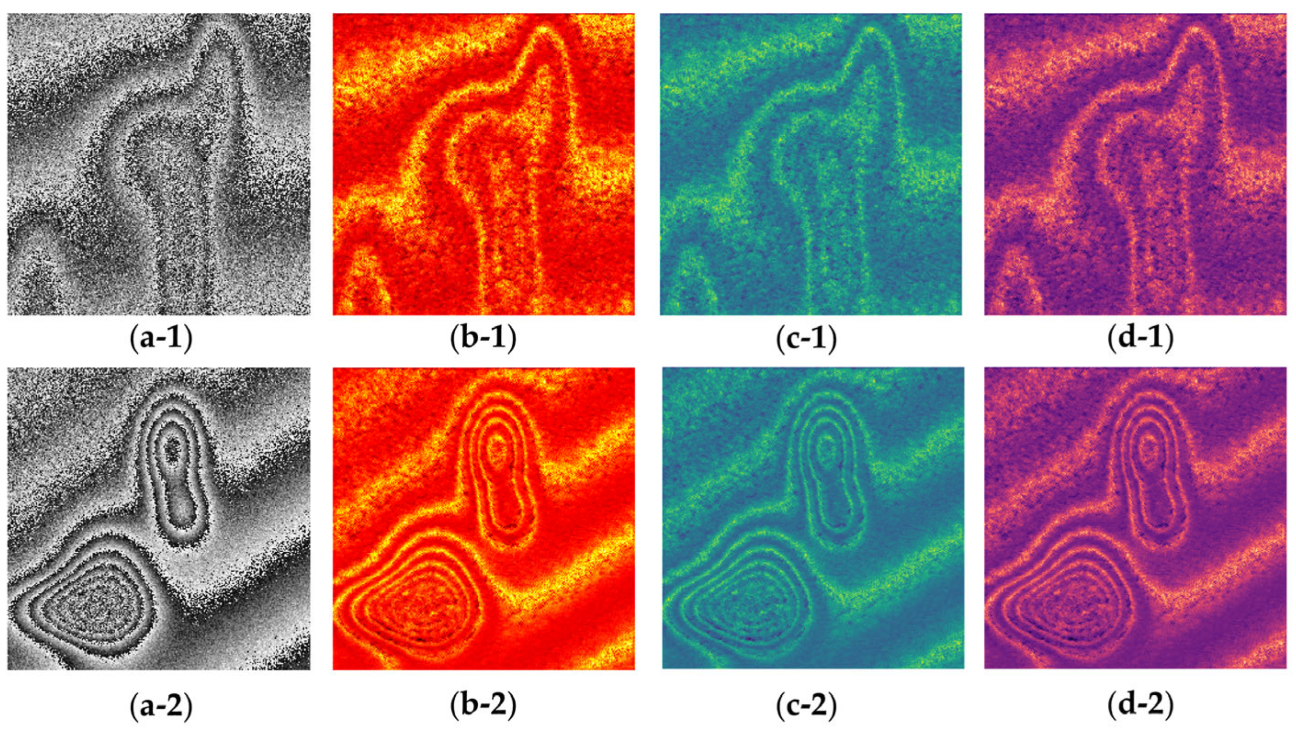
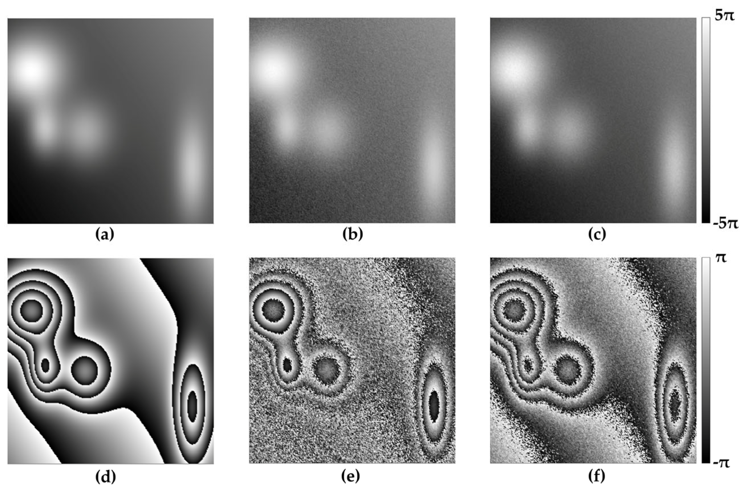
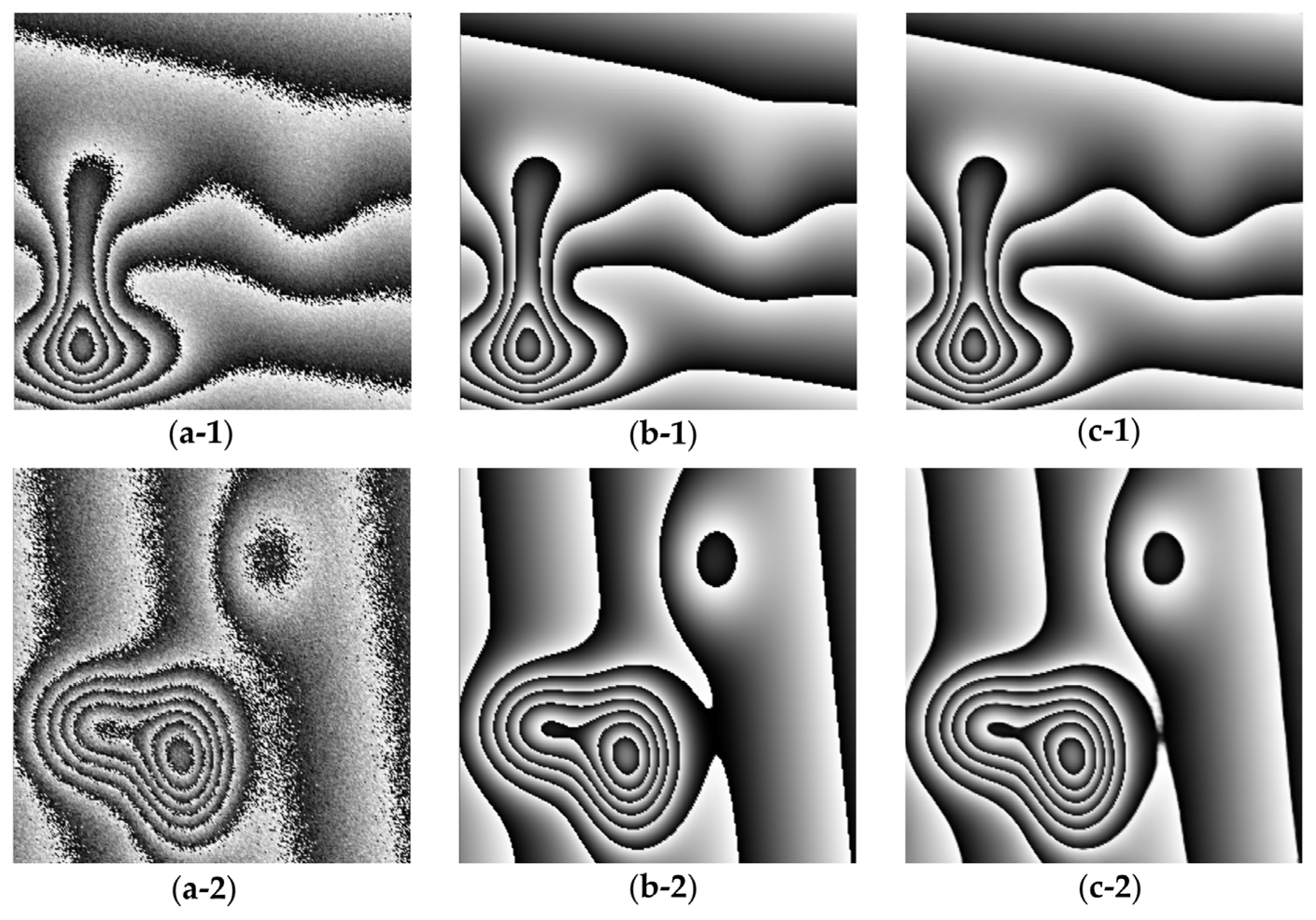
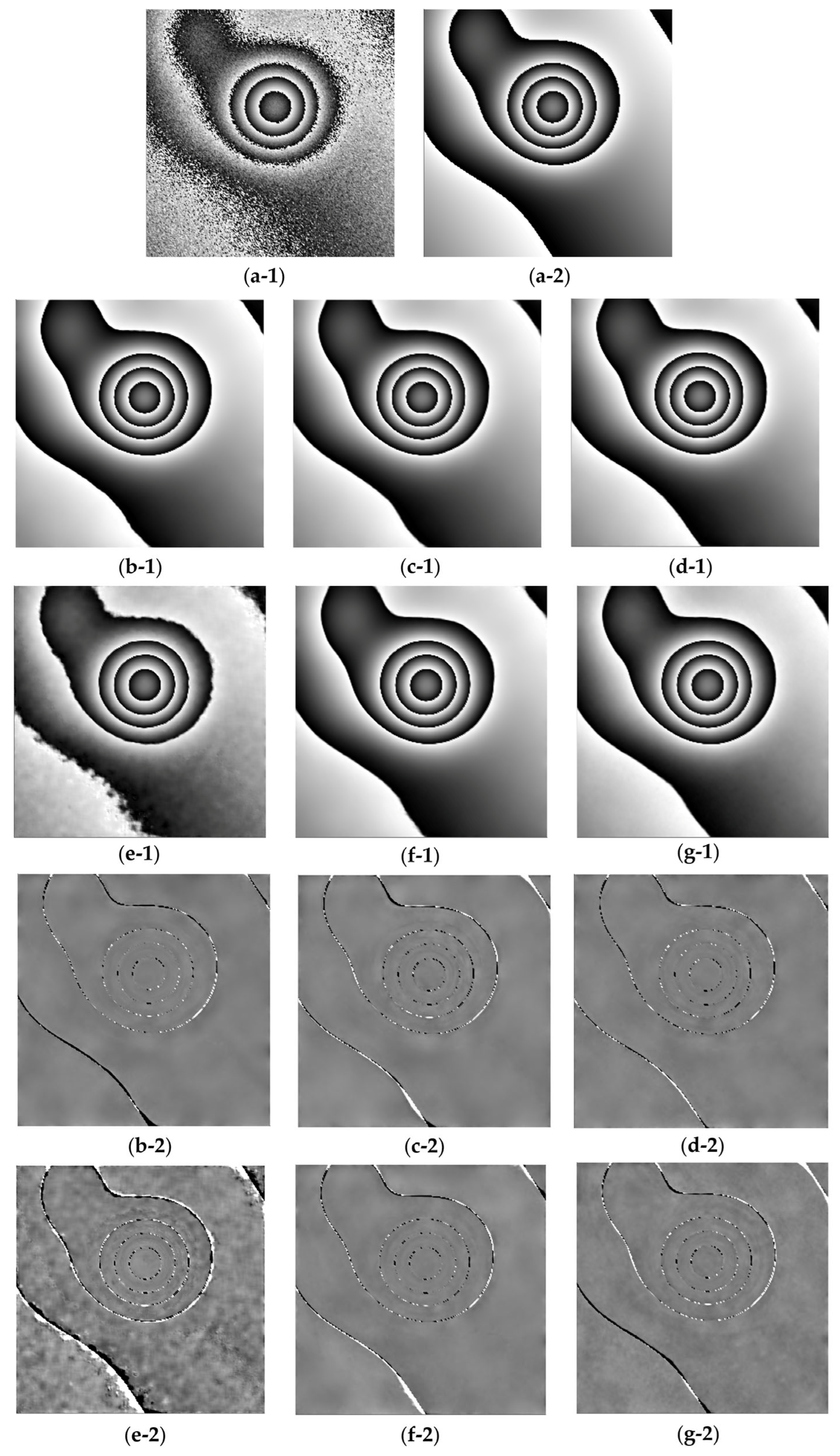
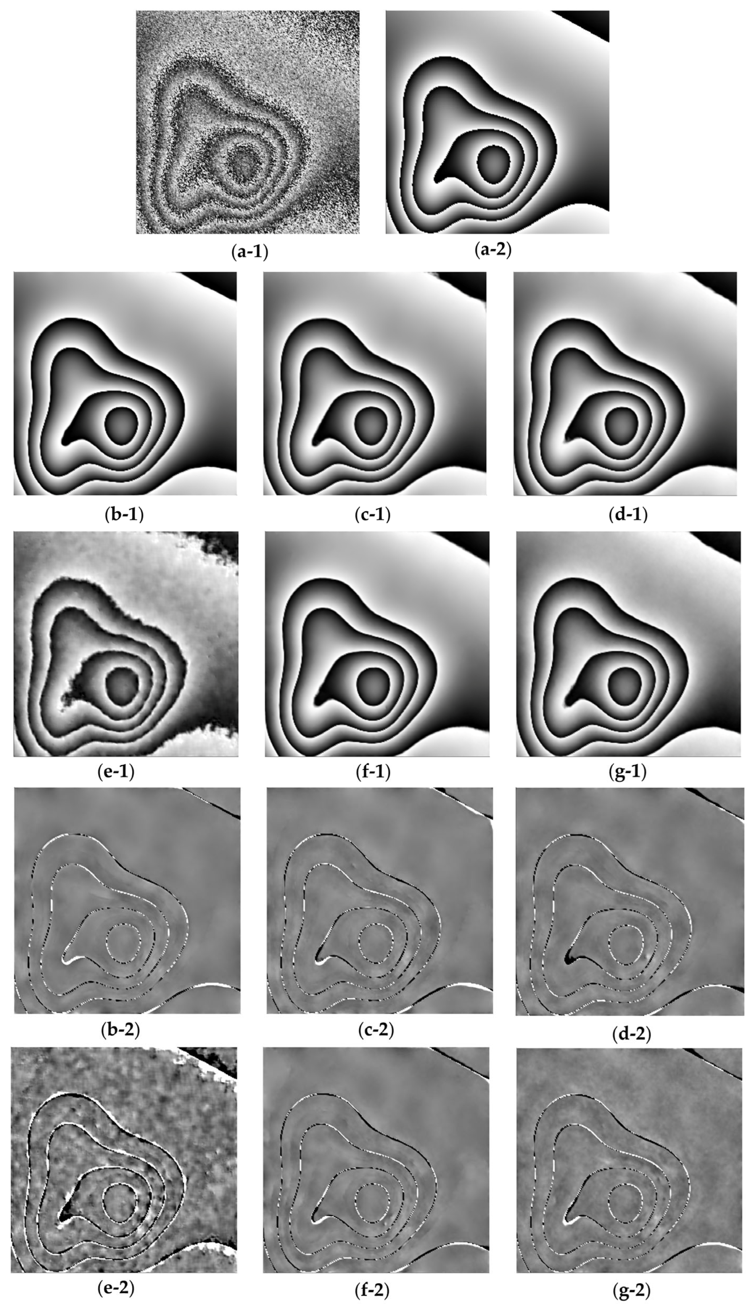
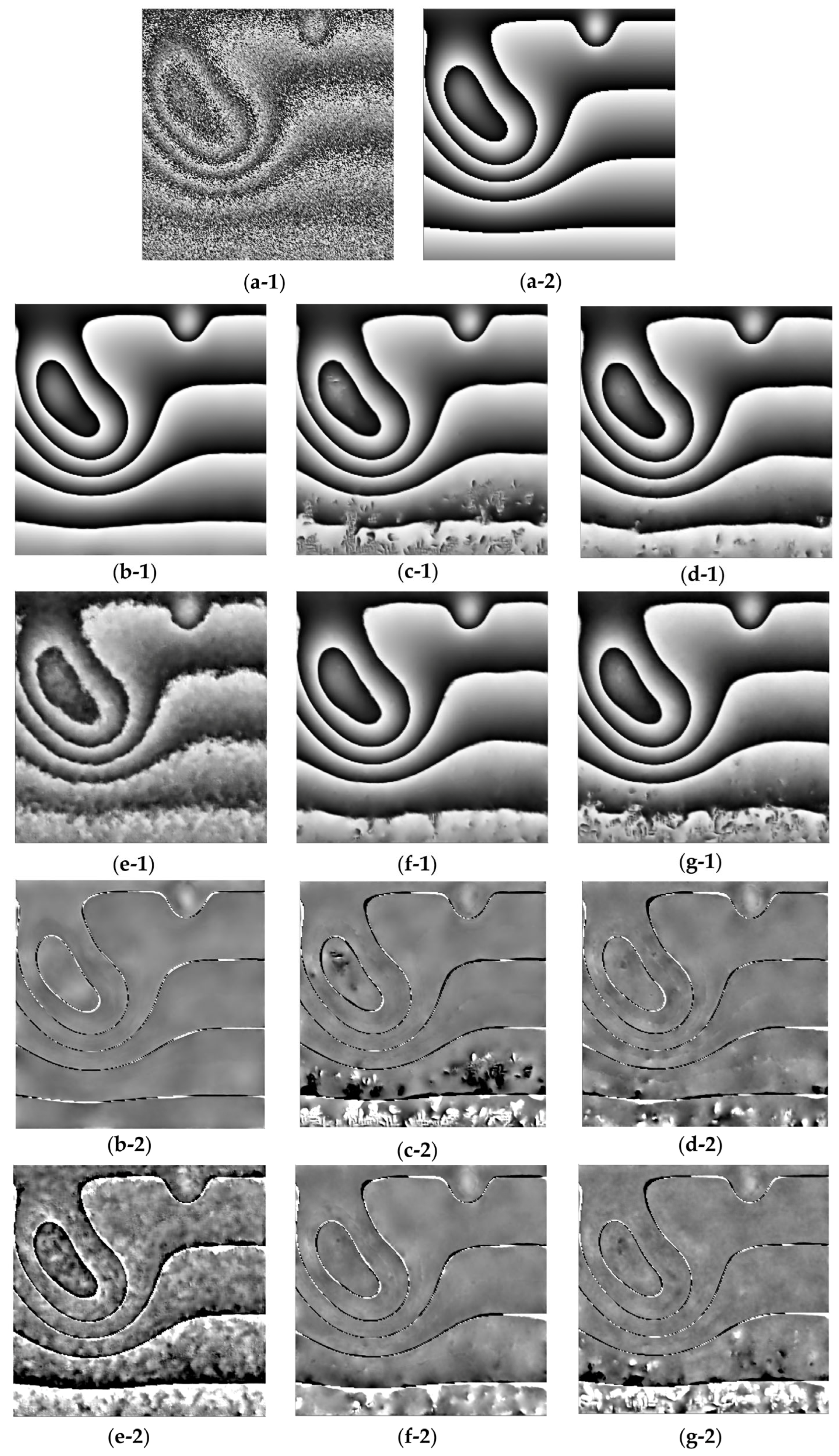
Out of 5000 images in each dataset, 4000 (80%) were used for training, 400 (10% of the training set) were held out as a validation set for early stopping and model selection, and 1000 (20%) were reserved for final testing. A consistent random selection method was applied to ensure reproducibility across experiments. Training was performed for 200 epochs using the Adam optimizer with an initial learning rate of 0.0001 and a batch size of 4. The learning rate was reduced by a factor of 0.5 every 50 epochs. The validation set was used for early stopping and model selection, with the final model chosen based on the lowest validation loss. Paired data: noisy wrapped-phase images I N and their corresponding clean noise-free images I NF were used for supervised training.
To quantitatively evaluate the performance of the network, we used MSE, PSNR, and SSIM as metrics. Each predicted denoised wrapped-phase image ( I DN ) was compared with its ground truth noise-free wrapped-phase image ( I NF ). MSE measures the average of the squared difference between the predicted and the ground truth wrapped-phase images. It provides an indication of reconstruction accuracy.
MSE = 1 M × N i = 1 M j = 1 N [ I DN i , j I NF i , j ] 2 .
where M and N represent the number of pixels in the image. A lower MSE indicates better denoising performance. PSNR measures the quality of the denoised image by assessing the error between I DN and I NF , and defined using MSE as:
PSNR = 10 log 10 ( MAX 2 MSE ) .
The parameter MAX is the maximum possible pixel value, set to 255 for grayscale images. A higher PSNR value indicates better image quality with less residual noise.
The SSIM evaluates the structural similarity between I DN and I NF by considering brightness, contrast, and structural differences. It is computed as:
SSIM I DN , I NF = l ( I DN , I NF ) α c ( I DN , I NF ) β s ( I DN , I NF ) γ .
The parameters α, β, and γ define the relative weights, while l I DN , I NF ,   c I DN , I NF , and s ( I DN , I NF ) represent luminance, contrast, and structure measures of I DN and I NF , respectively:
l I DN , I NF = 2 μ I DN μ I NF + C 1 μ I DN 2 + μ I NF 2 + C 1 c I DN , I NF = 2 σ I DN σ I NF + C 2 σ I DN 2 + σ I NF 2 + C 2 s I DN , I NF = σ I DN I NF + C 3 σ I DN σ I NF + C 3 .
where μ I DN and μ I NF represent the mean of I DN and I NF , respectively, and σ I DN and σ I NF are their variances. The term σ I DN I NF is the covariance between I DN and I NF , while C 1 , C 2 , and C 3 are small constants introduced to prevent a zero denominator during calculations:
c 1 = ( k 1 L ) 2 ,   c 2 = ( k 2 L ) 2 ,   c 3 = C 2 2
where L is the dynamic range of pixel values (255 for grayscale images), and k 1 and k 2 are small constants (usually less than 1).

4. Results

The proposed method is evaluated both qualitatively and quantitatively using computer-simulated and experimentally obtained wrapped-phase images. To assess its effectiveness, we train other deep learning-based networks, including DBDNet [26], DBDNet2 [27], AD-CNN [28], LGCT-Net [29], and LRDUNet [34], using the same training dataset and loss function as our model WPD-Net. The performance of each method is quantitatively measured using the metrics of MSE, PSNR, and SSIM. Additionally, real noisy phase images are analyzed qualitatively to further demonstrate the feasibility and practical applicability of our approach.

4.1. Experiments with Synthetic and Real Data

To assess the performance of WPD-Net, we evaluate it with two phase images randomly selected from the speckle noise dataset, each with different noise levels. Figure 5 presents two noisy wrapped-phase images: Figure 5(a-1) with moderate speckle noise (variance = 0.05) and Figure 5(a-2) with high speckle noise (variance = 0.08). Their corresponding clean noise-free ground truth images are shown in Figure 5(b-1) and Figure 5(b-2), respectively. The denoised outputs produced by WPD-Net are displayed in Figure 5(c-1,c-2), demonstrating that the network effectively suppresses speckle noise while preserving fine structural details, even under high noise conditions.
Next, we evaluate the effectiveness of WPD-Net with two other phase images selected from the Gaussian noise dataset. Figure 6 shows the input noisy wrapped-phase images: Figure 6(a-1) with moderate (SNR = 10 dB) and Figure 6(a-2) severe Gaussian noises (SNR = 5 dB). Their corresponding ground truth images are shown in Figure 6(b-1,b-2), while the denoised results produced by WPD-Net are displayed in Figure 6(c-1,c-2). The visual comparison demonstrates that WPD-Net effectively removes Gaussian noise while preserving fine structural details and maintaining phase continuity. Table 2 presents the performance metrics for simulated speckle noise and Gaussian noise.
We further compare WPD-Net with other deep learning-based methods for both speckle and Gaussian noise cases in Figure 7. For high-speckle noise (variance = 0.1), a wrapped-phase image is shown in Figure 7(a-1), alongside its corresponding clean noise-free image in Figure 7(a-2). The outputs produced by various methods are presented, including WPD-Net (Figure 7(b-1)), AD-CNN (Figure 7(c-1)), LGCT-Net (Figure 7(d-1)), DBDNet (Figure 7(e-1)), DBDNet2 (Figure 7(f-1)), and LRDUNet (Figure 7(g-1)). Their corresponding difference maps with respect to the ground truth are shown in Figure 7(b-2) through Figure 7(g-2), respectively. Due to the high noise level, DBDNet shows visible phase errors, especially around the areas that have large phase variations. In contrast, WPD-Net and other networks demonstrate better noise suppression and preserve structural consistency, as evidenced by the cleaner difference maps.
A similar comparison is performed for Gaussian noise with an SNR of 0 dB, as shown in Figure 8(a-1), with its corresponding clean noise-free image in Figure 8(a-2). The results denoised with other various methods are displayed: WPD-Net (Figure 8(b-1)), AD-CNN (Figure 8(c-1)), LGCT-Net (Figure 8(d-1)), DBDNet (Figure 8(e-1)), DBDNet2 (Figure 8(f-1)), and LRDUNet (g-1). Their respective difference maps are shown in Figure 8(b-2–g-2). Due to the significant intensity fluctuations caused by Gaussian noise, DBDNet and LGCT-Net show limitations in restoring phase continuity, resulting in visible artifacts. In contrast, WPD-Net and other networks achieve more effective noise reduction, ensuring improved phase consistency and reduced intensity distortion, as reflected in the corresponding difference maps.
Moreover, we evaluate the performance of the proposed method under a challenging mixed-noise scenario, consisting of high speckle noise (variance = 0.1) and Gaussian noise (SNR = 0 dB). As shown in Figure 9(a-1), the input wrapped-phase image is severely degraded, while the corresponding noise-free image is presented in Figure 9(a-2). The denoised results obtained from different methods are shown: WPD-Net (Figure 9(b-1)), AD-CNN (Figure 9(c-1)), LGCT-Net (Figure 9(d-1)), DBDNet (Figure 9(e-1)), DBDNet2 (Figure 9(f-1)), and LRDUNet (g-1), with their corresponding difference maps in Figure 9(b-2–g-2). It is important to emphasize that all compared networks were retrained using the same redesigned mixed-noise dataset as WPD-Net (see Section 3.2), ensuring a fair and consistent evaluation. Despite this, most methods struggle to fully remove noise, especially in areas with sharp transitions and boundaries, resulting in visible residual artifacts. In contrast, WPD-Net effectively reduced both speckle and Gaussian noise while preserving structural continuity and phase integrity. These visual results indicate that although careful dataset design contributes to improved performance, it alone is insufficient. Architectural enhancements are also necessary to achieve robust denoising under complex noise conditions. The superior performance of WPD-Net is attributed to its architectural innovations, particularly the integration of RDABs and the DFF module, which enables more effective multi-scale feature extraction and targeted noise suppression.
Table 3 presents the MSE, PSNR, and SSIM metrics for all networks shown in Figure 7, Figure 8 and Figure 9 providing a quantitative evaluation under both high speckle and Gaussian noise conditions. The results clearly demonstrate that WPD-Net achieves superior noise reduction while effectively preserving phase structure.
To further validate the effectiveness of our method, we evaluated WPD-Net on experimentally acquired wrapped-phase images using a full-field digital holographic interferometry setup. This setup enables the simultaneous capture of the entire surface of a sample in a single exposure, offering high-resolution phase information at a time without the need for mechanical scanning [39]. Two types of samples were tested: an acrylic plate and a PDMS (polydimethylsiloxane) specimen.
The acrylic sample, characterized by a relatively smooth and reflective surface, exhibited clear and continuous wrapped-phase fringes with a moderate noise level. The experimentally acquired noisy wrapped-phase image, having an SNR of 6.57 dB, is shown in Figure 10(a-1). The denoised results are presented in Figure 10(b-1–g-1), using WPD-Net, AD-CNN, LGCT-Net, DBDNet, DBDNet2, and LRDUNet, respectively. The WPD-Net output shows the highest quality restoration with improved clarity and reduced noise, while other methods leave visible residual noise or artifacts.
We further imaged a PDMS sample, which presented a much more challenging case due to its highly non-uniform and elastic surface. This led to densely packed and irregular wrapped-phase patterns, making noise suppression particularly difficult. The noisy wrapped-phase image for PDMS with an SNR of 6.52 dB is shown in Figure 10(a-2). The denoising results using the various methods are displayed in Figure 10(b-2–g-2). While all methods attempted to restore the phase pattern, WPD-Net most effectively suppressed the complex noise and preserved the fine structural details of the wrap contours. Competing methods struggled to fully denoise the image and exhibited artifacts, particularly around high-gradient regions.
To further challenge the denoising capabilities of WPD-Net, we imaged an additional PDMS sample that had water droplets on it and boundary leaks. This scenario introduced phase discontinuities, disconnected wrap lines, and sharp phase transitions, rather than only dense wrapping. The noisy wrapped-phase image used for this case, with an SNR of 4.79 dB, is shown in Figure 10(a-3). The corresponding denoised outputs using the same set of methods are illustrated in Figure 10(b-3–g-3). Despite the highly irregular nature of this sample, WPD-Net demonstrated robust performance, effectively recovering the structural layout of the phase wraps while minimizing noise. While LGCT-Net and LRDUNet showed some success, other models failed to handle the noise complexity and discontinuities.
Overall, these experimental results confirm that WPD-Net is not only effective on synthetic data but also reliable with real-world interferometric data. Its ability to generalize to challenging environments, including sharp transitions, disconnected phase regions, and irregular surface profiles, highlights its practical utility in wrapped-phase image denoising tasks.

4.2. Ablation Study

An ablation study was conducted using synthetic data to evaluate the individual contributions of key components within the proposed network. The evaluation used 750 test images in total: 250 each from the speckle noise, Gaussian noise, and combined noise datasets (with speckle variance = 0.1 and Gaussian SNR = 0 dB). The study began by testing the effect of training with only the MSE loss function. Subsequently, we evaluated architectural configurations, including: (i) a model with RDABs but without the DFF module, (ii) a model with RDBs but without attention, and (iii) the full WPD-Net, which includes the SFE module, RDABs, DFF module, and the dynamic hybrid loss function combining MSE and SSIM.
Quantitative results in Table 4 show that the complete WPD-Net consistently outperformed the other variants in terms of MSE, PSNR, and SSIM. Visual comparisons are also presented in Figure 11 using one representative test sample. The figure includes: Figure 11(a-1) the noisy wrapped-phase input image, Figure 11(a-2) its ground truth, Figure 11(b-1) denoised output using MSE loss, Figure 11(c-1) a model with RDABs but without DFF module, Figure 11(d-1) a model with RDB but without attention, Figure 11(e-1) the final WPD-Net output, and Figure 11(b-2–e-2) the corresponding difference maps.
The visual results demonstrate that attention mechanisms in RDABs enable the network to emphasize structurally relevant regions, while the DFF module improves global feature fusion. The combined effect of these components—along with the dynamic hybrid loss—leads to enhanced denoising, sharper phase recovery, and progressive suppression of residual noise and artifacts. Together, these findings provide strong quantitative and qualitative evidence of the importance of attention, feature fusion, and dynamic loss optimization in achieving high-performance wrapped-phase denoising with WPD-Net.

4.3. Model Complexity

In Table 5, we compare the model complexity of WPD-Net with other state-of-the-art denoising networks, including DBDNet, DBDNet2, AD-CNN, LGCT-Net, and LRDUNet, in terms of the number of parameters, floating-point operations (FLOPs), and inference time. WPD-Net demonstrates the lowest parameter count (0.859 million) and the fewest FLOPs (225.1 million), while also achieving the fastest inference time (21.19 ms) on 256 × 256 images. This efficiency is achieved through its lightweight design that integrates shallow feature extraction, RDABs, and dense feature fusion, avoiding the need for computationally intensive encoder–decoder architectures or transformer-based modules.
Comparison models, DBDNet and DBDNet2, utilize dilated convolutional blocks to expand the receptive field without pooling, enabling better handling of high-speckle noise. However, this comes at the cost of increased computational complexity, with DBDNet requiring 298.9 million FLOPs and DBDNet2 slightly increased to 341.3 million. Despite their relatively modest parameter counts, both models are slower than WPD-Net. AD-CNN and LGCT-Net lead to higher complexity, with AD-CNN reaching 421.2 million FLOPs and LGCT-Net the highest among all at 859.7 million, primarily due to their deeper networks and the inclusion of transformer-style attention in LGCT-Net. LRDUNet attempts to achieve a lower parameter count using grouped convolutions and dense skip connections, but still results in 276.8 million FLOPs and longer inference time compared to WPD-Net.
Our proposed WPD-Net achieves an optimal balance between denoising performance and computational efficiency, making it particularly well-suited for real-time and resource-constrained applications, such as embedded biomedical imaging systems.

5. Discussion

WPD-Net, a deep learning architecture has been proposed for denoising wrapped-phase images under severe speckle, Gaussian, and mixed noise conditions. The network employs multi-scale feature extraction and attention mechanisms to focus on relevant spatial and channel details while maintaining phase continuity. Combined with a dynamic hybrid loss function, these design choices enable robust noise suppression while preserving structural integrity.
The experiments conducted with both synthetic and real datasets confirm that WPD-Net consistently delivers high-quality denoising results. This not only enhances reconstruction accuracy but also ensures reliable inputs for downstream tasks such as phase unwrapping. While many existing deep learning-based phase unwrapping methods attempt to jointly denoise and unwrap phase images, they typically require large and diverse training datasets [40,41,42], along with long training durations—often exceeding 10 h [39]. Moreover, their performance can deteriorate significantly when exposed to complex mixed noise. In contrast, our two-stage approach—first applying WPD-Net for denoising, followed by a simple unwrapping algorithm—offers better adaptability, lower computational cost, and faster inference. As a lightweight model with significantly fewer parameters than conventional joint models, WPD-Net reduces training time to under two hours and achieves real-time inference (21.19 ms per image), making it well-suited for practical applications where both accuracy and speed are critical.
To visualize the effectiveness of this workflow, 3D surface plots of unwrapped-phase images are shown in Figure 12. For both the acrylic and PDMS samples used in Figure 10(a-1,a-2), the combination of WPD-Net and a basic 2D unwrapping method produces clean and coherent 3D surfaces, comparable to the outputs from recent end-to-end phase unwrapping networks like DenSFA-PU [39] and U2-Net [42]. These results highlight the practical value of separating denoising and unwrapping stages when using a highly capable denoising model like WPD-Net. While we demonstrated WPD-Net’s ability to produce visually accurate unwrapped-phase results, a detailed quantitative assessment of the unwrapping accuracy using different denoising methods was not performed, as the primary focus of this study was on wrapped-phase denoising.
Nevertheless, a limitation remains under extreme noise conditions (SNR < 0 dB). Although WPD-Net performs robustly at an SNR of 0 dB, its performance may deteriorate when the noise power exceeds the signal, limiting the network’s ability to recover meaningful information. In future work, we aim to address this challenge by incorporating training strategies that account for temporal dynamics or large missing regions, thereby improving both robustness and generalization. Additionally, we plan to introduce phase unwrapping accuracy metrics, such as NRMSE or unwrapping error rate, to quantitatively evaluate the effectiveness of WPD-Net-enabled workflows compared to those using other denoising methods.

6. Conclusions

In this paper, we have proposed a deep learning-based framework named WPD-Net for denoising wrapped-phase images heavily affected by speckle, Gaussian, or mixed noise. The architecture, composed of Shallow Feature Extraction (SFE), Residual Dense Attention Blocks (RDABs), and a Dense Feature Fusion (DFF) module, was specifically designed to enhance noise suppression while preserving the structural integrity and continuity of phase patterns. Additionally, we introduced a dynamic hybrid loss function to guide the network in achieving better reconstruction accuracy. Extensive evaluations on both synthetic and experimental datasets showed that WPD-Net consistently outperformed existing state-of-the-art models, including DBDNet, DBDNet2, AD-CNN, LGCT-Net, and LRDUNet, in terms of metrics such as MSE, PSNR, and SSIM. Furthermore, the network demonstrated strong generalization ability across different noise conditions.

Author Contributions

Conceptualization, M.A. and B.L.; methodology, M.A.; software, M.A. and Y.K.; formal analysis, M.A. and B.L.; investigation, M.A., T.Y. and W.C.; resources, M.A., Y.K., and B.L.; data curation, M.A. and T.Y.; writing—original draft preparation, M.A. and B.L.; writing—review and editing, M.A., Y.K., T.Y., W.C. and B.L.; visualization, M.A. All authors have read and agreed to the published version of the manuscript.

Funding

This work was supported by the Technology Innovation Program (20021979) funded by the Ministry of Trade, Industry, and Energy (MOTIE), and the Basic Science Research Program through the National Research Foundation of Korea (NRF) funded by the Ministry of Education (RS-2024–00461205).

Institutional Review Board Statement

Not applicable.

Informed Consent Statement

Not applicable.

Data Availability Statement

The data presented in this study are available on request from the corresponding author. The data are not publicly available due to privacy or ethical restrictions.

Acknowledgments

The authors would like to thank Chi-Ok Hwang for his valuable support in handling the deep learning-based neural networks. His assistance greatly contributed to the technical development of this work.

Conflicts of Interest

The authors declare no conflicts of interest.

References

  1. Wyant, J.C. Dynamic Interferometry. Opt. Photonics News 2003, 14, 36–41. [Google Scholar] [CrossRef]
  2. Ghiglia, D.C. Two-Dimensional Phase Unwrapping: Theory, Algorithms and Software; Wiley: Hoboken, NJ, USA, 1998. [Google Scholar]
  3. Huntley, J.M. Random Phase Measurement Errors in Digital Speckle Pattern Interferometry. Opt. Lasers Eng. 1997, 26, 131–150. [Google Scholar] [CrossRef]
  4. Aebischer, A.H.; Waldner, S. A Simple and Effective Method for Filtering Speckle-Interferometric Phase Fringe Patterns. Opt. Commun. 1999, 162, 205–210. [Google Scholar] [CrossRef]
  5. Goodman, J.W. Speckle Phenomena in Optics: Theory and Applications; Roberts and Company Publishers: Greenwood Village, CO, USA, 2007. [Google Scholar]
  6. Montresor, S.; Picart, P. Quantitative Appraisal for Noise Reduction in Digital Holographic Phase Imaging. Opt. Express 2016, 24, 14322–14343. [Google Scholar] [CrossRef]
  7. Piniard, M.; Sorrente, B.; Hug, G.; Picart, P. Theoretical Analysis of Surface-Shape-Induced Decorrelation Noise in Multi-Wavelength Digital Holography. Opt. Express 2021, 29, 14720–14735. [Google Scholar] [CrossRef]
  8. Montresor, S.; Picart, P. On the Assessment of De-Noising Algorithms in Digital Holographic Interferometry and Related Approaches. Appl. Phys. B 2022, 128, 59. [Google Scholar] [CrossRef]
  9. Kemao, Q. Windowed Fourier Transform for Fringe Pattern Analysis. Appl. Opt. 2004, 43, 2695–2702. [Google Scholar] [CrossRef]
  10. Kemao, Q. Two-Dimensional Windowed Fourier Transform for Fringe Pattern Analysis: Principles, Applications and Implementations. Opt. Lasers Eng. 2007, 45, 304–317. [Google Scholar] [CrossRef]
  11. O’Shea, K.; Nash, R. An Introduction to Convolutional Neural Networks. arXiv 2015, arXiv:1511.08458. [Google Scholar]
  12. Wang, P.; Zhang, H.; Patel, V.M. SAR Image Despeckling Using a Convolutional Neural Network. IEEE Signal Process. Lett. 2017, 24, 1763–1767. [Google Scholar] [CrossRef]
  13. Jeon, W.; Jeong, W.; Son, K.; Yang, H. Speckle Noise Reduction for Digital Holographic Images Using Multi-Scale Convolutional Neural Networks. Opt. Lett. 2018, 43, 4240–4243. [Google Scholar] [CrossRef]
  14. Zhang, Q.; Yuan, Q.; Li, J.; Yang, Z.; Ma, X. Learning a Dilated Residual Network for SAR Image Despeckling. Remote Sens. 2018, 10, 196. [Google Scholar] [CrossRef]
  15. Choi, G.; Ryu, D.; Jo, Y.; Kim, Y.; Park, W.; Min, H.S.; Park, Y. Cycle-Consistent Deep Learning Approach to Coherent Noise Reduction in Optical Diffraction Tomography. Opt. Express 2019, 27, 4927–4943. [Google Scholar] [CrossRef]
  16. Wang, M.; Zhu, W.; Yu, K.; Chen, Z.; Shi, F.; Zhou, Y.; Ma, Y.; Peng, Y.; Bao, D.; Feng, S.; et al. Semi-Supervised Capsule cGAN for Speckle Noise Reduction in Retinal OCT Images. IEEE Trans. Med. Imaging 2021, 40, 1168–1183. [Google Scholar] [CrossRef] [PubMed]
  17. Yan, K.; Yu, Y.; Sun, T.; Asundi, A.; Kemao, Q. Wrapped Phase Denoising Using Convolutional Neural Networks. Opt. Lasers Eng. 2020, 128, 105999. [Google Scholar] [CrossRef]
  18. Zhang, K.; Zuo, W.; Chen, Y.; Meng, D.; Zhang, L. Beyond a Gaussian Denoiser: Residual Learning of Deep CNN for Image Denoising. IEEE Trans. Image Process. 2017, 26, 3142–3155. [Google Scholar] [CrossRef]
  19. Lin, B.; Fu, S.; Zhang, C.; Wang, F.; Li, Y. Optical Fringe Patterns Filtering Based on Multi-Stage Convolution Neural Network. Opt. Lasers Eng. 2020, 126, 105853. [Google Scholar] [CrossRef]
  20. Figueroa, A.R.; Flores, V.H.; Rivera, M. Deep Neural Network for Fringe Pattern Filtering and Normalization. Appl. Opt. 2021, 60, 2022–2036. [Google Scholar] [CrossRef]
  21. Montresor, S.; Tahon, M.; Laurent, A.; Picart, P. Computational De-Noising Based on Deep Learning for Phase Data in Digital Holographic Interferometry. APL Photonics 2020, 5, 030801. [Google Scholar] [CrossRef]
  22. Fang, Q.; Xia, H.; Song, Q.; Zhang, M.; Guo, R.; Montresor, S.; Picart, P. Speckle Denoising Based on Deep Learning via a Conditional Generative Adversarial Network in Digital Holographic Interferometry. Opt. Express 2022, 30, 20666–20683. [Google Scholar] [CrossRef]
  23. Yan, K.; Chang, L.; Andrianakis, M.; Tornari, V.; Yu, Y. Deep Learning-Based Wrapped Phase Denoising Method for Application in Digital Holographic Speckle Pattern Interferometry. Appl. Sci. 2020, 10, 4044. [Google Scholar] [CrossRef]
  24. Fang, Q.; Li, Q.; Song, Q.; Montresor, S.; Picart, P.; Xia, H. Convolutional and Fourier Neural Networks for Speckle Denoising of Wrapped Phase in Digital Holographic Interferometry. Opt. Commun. 2024, 550, 129955. [Google Scholar] [CrossRef]
  25. Zhang, H.; Huang, D.; Wang, K. Denoising of Wrapped Phase in Digital Speckle Shearography Based on Convolutional Neural Network. Appl. Sci. 2024, 14, 4135. [Google Scholar] [CrossRef]
  26. Li, J.; Tang, C.; Xu, M.; Fan, Z.; Lei, Z. DBDNet for Denoising in ESPI Wrapped Phase Patterns with High Density and High Speckle Noise. Appl. Opt. 2021, 60, 10070–10079. [Google Scholar] [CrossRef] [PubMed]
  27. Li, J.; Tang, C.; Xu, M.; Lei, Z. Uneven Wrapped Phase Pattern Denoising Using a Deep Neural Network. Appl. Opt. 2022, 61, 7150–7157. [Google Scholar] [CrossRef]
  28. Wang, L.; Li, R.; Tian, F.; Fang, X. Application of Attention-DnCNN for ESPI Fringe Patterns Denoising. J. Opt. Soc. Am. A 2022, 39, 2110–2123. [Google Scholar] [CrossRef]
  29. He, H.; Tang, C.; Liu, L.; Zhang, L.; Lei, Z. Generalized Denoising Network LGCT-Net for Various Types of ESPI Wrapped Phase Patterns. J. Opt. Soc. Am. A 2024, 41, 1664–1674. [Google Scholar] [CrossRef]
  30. Vaswani, A.; Shazeer, N.; Parmar, N.; Uszkoreit, J.; Jones, L.; Gomez, A.N.; Kaiser, Ł.; Polosukhin, I. Attention Is All You Need. Adv. Neural Inf. Process. Syst. 2017, 30, 5998–6008. [Google Scholar]
  31. Yu, H.; Yang, T.; Zhou, L.; Wang, Y. PDNet: A Lightweight Deep Convolutional Neural Network for InSAR Phase Denoising. IEEE Trans. Geosci. Remote Sens. 2022, 60, 5239309. [Google Scholar] [CrossRef]
  32. Hao, F.; Tang, C.; Xu, M.; Lei, Z. Batch Denoising of ESPI Fringe Patterns Based on Convolutional Neural Network. Appl. Opt. 2019, 58, 3338–3346. [Google Scholar] [CrossRef]
  33. Xu, M.; Tang, C.; Hong, N.; Lei, Z. MDD-Net: A Generalized Network for Speckle Removal with Structure Protection and Shape Preservation for Various Kinds of ESPI Fringe Patterns. Opt. Lasers Eng. 2022, 154, 107017. [Google Scholar] [CrossRef]
  34. Gurrola-Ramos, J.; Dalmau, O.; Alarcón, T. U-Net Based Neural Network for Fringe Pattern Denoising. Opt. Lasers Eng. 2022, 149, 106829. [Google Scholar] [CrossRef]
  35. Yan, K.; Yu, Y.; Huang, C.; Sui, L.; Qian, K.; Asundi, A. Fringe Pattern Denoising Based on Deep Learning. Opt. Commun. 2019, 437, 148–152. [Google Scholar] [CrossRef]
  36. Glorot, X.; Bordes, A.; Bengio, Y. Deep Sparse Rectifier Neural Networks. In Proceedings of the Fourteenth International Conference on Artificial Intelligence and Statistics (AISTATS), Fort Lauderdale, FL, USA, 11–13 April 2011; JMLR W&CP. pp. 315–323. [Google Scholar]
  37. Park, J.; Woo, S.; Lee, J.Y.; Kweon, I.S. BAM: A Simple and Lightweight Attention Module for Convolutional Neural Networks. Int. J. Comput. Vis. 2020, 128, 783–798. [Google Scholar] [CrossRef]
  38. Ioffe, S.; Szegedy, C. Batch Normalization: Accelerating Deep Network Training by Reducing Internal Covariate Shift. In Proceedings of the International Conference on Machine Learning (ICML), Lille, France, 7–9 July 2015; PMLR: London, UK, 2015; pp. 448–456. [Google Scholar]
  39. Awais, M.; Yoon, T.; Hwang, C.O.; Lee, B. DenSFA-PU: Learning to Unwrap Phase in Severe Noisy Conditions. Opt. Laser Technol. 2025, 187, 112757. [Google Scholar] [CrossRef]
  40. Wang, K.; Li, Y.; Kemao, Q.; Di, J.; Zhao, J. One-Step Robust Deep Learning Phase Unwrapping. Opt. Express 2019, 27, 15100–15115. [Google Scholar] [CrossRef]
  41. Qin, Y.; Wan, S.; Wan, Y.; Weng, J.; Liu, W.; Gong, Q. Direct and Accurate Phase Unwrapping with Deep Neural Network. Appl. Opt. 2020, 59, 7258–7267. [Google Scholar] [CrossRef]
  42. Chen, J.; Kong, Y.; Zhang, D.; Fu, Y.; Zhuang, S. Two-Dimensional Phase Unwrapping Based on U2-Net in Complex Noise Environment. Opt. Express 2023, 31, 29792–29812. [Google Scholar] [CrossRef]
Figure 1. (a) Architecture of the proposed WPD-Net, which comprises a shallow feature extraction (SFE) module, residual dense attention Blocks (RDABs), and dense feature fusion (DFF) module with global residual learning. (b) Detailed structure of RDAB, including local residual learning and both channel and spatial attention mechanisms.
Applsci 15 05514 g001
Figure 2. Visualization of attention maps from the first RDAB layer in WPD-Net for two representative noisy wrapped-phase images. (a-1,a-2) Input noisy images; (b-1,b-2) Spatial attention maps showing key regions affected by noise or sharp transitions; (c-1,c-2) Up-sampled channel attention vectors; (d-1,d-2) Combined attention maps obtained by summing spatial and channel attention maps.
Applsci 15 05514 g002
Figure 3. Example of synthetically generated data. The true phase image is presented (a) without noise, (b) with speckle noise, and (c) with Gaussian noise. The corresponding wrapped-phase images are shown (d) without noise, (e) with speckle noise (variance = 0.1), and (f) with Gaussian noise (SNR 5 dB). Each image consists of 256 × 256 pixels.
Applsci 15 05514 g003
Figure 4. Training and testing process of WPD-Net. Paired sets of noisy wrapped-phase images and clean noise-free images were used for training. The total dataset consists of 5000 images, with 4000 allocated for training and 1000 for testing.
Applsci 15 05514 g004
Figure 5. Denoising performance on simulated wrapped-phase images with speckle noise. (a-1,a-2) Noisy input images with moderate (variance = 0.05) and high (variance = 0.08) speckle noise, respectively; (b-1,b-2) Corresponding ground truth images; (c-1,c-2) Denoised outputs from WPD-Net.
Applsci 15 05514 g005
Figure 6. Denoising performance on simulated wrapped-phase images with Gaussian noise. (a-1,a-2) Noisy input images with moderate (SNR = 10 dB) and severe (SNR = 5 dB) Gaussian noise, respectively; (b-1,b-2) Corresponding ground truth images; (c-1,c-2) Denoised outputs from WPD-Net.
Applsci 15 05514 g006
Figure 7. Comparison of denoising performance on wrapped-phase images with severe speckle noise (Variance = 0.1). (a-1) shows the input noisy wrapped-phase image, and (a-2) shows the corresponding clean ground truth. The denoised results and their corresponding difference maps are shown for each method: WPD-Net in (b-1,b-2), AD-CNN in (c-1,c-2), LGCT-Net in (d-1,d-2), DBDNet in (e-1,e-2), DBDNet2 in (f-1,f-2), and LRDUNet in (g-1,g-2).
Applsci 15 05514 g007
Figure 8. Comparison of denoising performance on wrapped-phase images with severe Gaussian noise (SNR = 0 dB). (a-1) shows the input noisy wrapped-phase image, while (a-2) shows the corresponding clean ground truth. The denoised outputs and their difference maps are provided for WPD-Net (b-1,b-2), AD-CNN (c-1,c-2), LGCT-Net (d-1,d-2), DBDNet (e-1,e-2), DBDNet2 (f-1,f-2), and LRDUNet (g-1,g-2).
Applsci 15 05514 g008
Figure 9. Comparison of denoising performance on wrapped-phase images with combined speckle (Variance = 0.1) and Gaussian (SNR = 0 dB) noise. (a-1) shows the input noisy wrapped-phase image, while (a-2) presents the corresponding clean ground truth. The denoised results and their difference maps are shown for WPD-Net (b-1,b-2), AD-CNN (c-1,c-2), LGCT-Net (d-1,d-2), DBDNet (e-1,e-2), DBDNet2 (f-1,f-2), and LRDUNet (g-1,g-2).
Applsci 15 05514 g009
Figure 10. Experimental denoising results on wrapped-phase images acquired using full-field digital holographic interferometry. (a-1) Noisy wrapped-phase image of an acrylic sample, with SNR = 6.57 dB. (a-2) Noisy input of a PDMS sample with dense wraps and a complex surface profile, with SNR = 6.52 dB. (a-3) Noisy input of a challenging PDMS case with leaky boundaries and discontinuous wraps, with SNR = 4.79 dB. Denoised outputs are shown for (b-1b-3) WPD-Net, (c-1c-3) AD-CNN, (d-1d-3) LGCT-Net, (e-1e-3) DBDNet, (f-1f-3) DBDNet2, and (g-1g-3) LRDUNet.
Applsci 15 05514 g010
Figure 11. Visual results of the ablation study comparing different architectural and training configurations of WPD-Net. (a-1) Noisy wrapped-phase input image; (a-2) ground truth; (b-1) denoised result using only MSE loss; (c-1) result with RDABs but without the DFF module; (d-1) output from the model with residual dense blocks (RDBs) and no attention; (e-1) output from the complete WPD-Net with SFE, RDABs, DFF, and dynamic hybrid loss. Corresponding difference maps with respect to ground truth are shown in (b-2e-2).
Applsci 15 05514 g011
Figure 12. 3D surface plots of the phase images unwrapped from the inputs shown in Figure 10(a-1,a-2). For the acrylic sample: (a-1) result obtained using WPD-Net denoising followed by a simple 2D phase unwrapping algorithm, (a-2) result from DenSFA-PU, and (a-3) result from U2-Net. For the PDMS sample: (b-1) result from WPD-Net with basic unwrapping, (b-2) result from DenSFA-PU, and (b-3) result from U2-Net result.
Applsci 15 05514 g012
Table 1. Detailed configuration of proposed network layers.
LayerFeature Map (H × W × C)PaddingDilation
Input256 × 256 × 1--
Shallow Feature Extraction (Conv C ReLU) 256 × 256 × 4811
Residual Dense Attention Block 1 (RDAB1)256 × 256 × 2411
Residual Dense Attention Block 2 (RDAB2)256 × 256 × 2411
Residual Dense Attention Block 3 (RDAB3)256 × 256 × 2411
Residual Dense Attention Block 4 (RDAB4)256 × 256 × 2411
Global Feature Fusion (1 × 1 Conv)256 × 256 × 4811
Global Feature Fusion (3 × 3 Conv)256 × 256 × 4811
Global Residual Learning
(Residual Connection)
256 × 256 × 4811
Final Convolution (Output Layer)256 × 256 × 111
Table 2. Quantitative metrics for simulated wrapped-phase patterns with different noises.
SamplesMSEPSNRSSIM
Image with Speckle noise
of Variance 0.05
0.005627.680.989
Image with Speckle noise
of Variance 0.08
0.006926.930.979
Image with Gaussian noise
of SNR 10
0.006227.570.981
Image with Gaussian noise
of SNR 5
0.007325.720.975
Table 3. Quantitative comparison of simulated wrapped-phase patterns (Figure 7, Figure 8 and Figure 9).
MethodsSpeckle NoiseGaussian NoiseCombined Noise
MSEPSNRSSIMMSEPSNRSSIMMSEPSNRSSIM
DBDNet [26]0.035118.6740.8840.041217.9350.8270.21638.5360.621
DBDNet2 [27]0.010322.4550.9630.018522.4760.9580.085219.7450.863
AD-CNN [28]0.009825.0360.9740.010624.9620.9710.098317.6270.826
LGCT-Net [29]0.014621.9450.9530.028420.8540.9330.061720.5290.857
LRDUNet [34]0.008224.0150.9750.015323.7110.9640.099418.2620.878
WPD-Net0.006826.5860.9870.008525.9810.9730.013523.8710.959
Table 4. Results of ablation study.
MSEPSNRSSIM
WPD-Net with MSE loss0.029816.3350.816
With RDAB and no DFF module0.017320.1080.884
With RDB and no attention0.014921.8340.913
Our proposed0.007626.1640.982
Table 5. Model complexity comparison and running time of models on 256 × 256 image pixels.
ModelsParameters (Millions)FLOPs
(Millions)
Run Time
(ms)
DBDNet [26]0.988 298.926.30
DBDNet2 [27]0.951 341.327.61
AD-CNN [28]1.637 421.229.58
LGCT-Net [29]8.796 859.751.39
LRDUNet [34]4.213 276.832.74
WPD-Net0.859 225.121.19
Disclaimer/Publisher’s Note: The statements, opinions and data contained in all publications are solely those of the individual author(s) and contributor(s) and not of MDPI and/or the editor(s). MDPI and/or the editor(s) disclaim responsibility for any injury to people or property resulting from any ideas, methods, instructions or products referred to in the content.

