Multi-Attribute Collaborative Optimization for Multimodal Transportation Based on User Preferences

Abstract

Given the differing interests and demands of various participants in multimodal transportation, this paper proposes a multi-attribute decision-making method driven by user preferences. Firstly, a four-dimensional optimization model is established with the objectives of minimizing transportation costs, transportation time, carbon emissions, and transportation risks. Furthermore, considering the practical aspects of transportation, differentiated time window constraints are designed based on the continuous time windows of highway transportation, railway train schedules, and the arrival and departure time characteristics of waterway vessels. In terms of solution methods, an improved Genetic Algorithm (GA) and Aptenodytes Forsteri Optimization (AFO) hybrid algorithm (GA-AFO) is proposed, which introduces GA to generate a high-quality initial population to accelerate convergence. By replacing the traditional gradient estimation strategy with a random mutation strategy based on probability distribution, the local search mechanism of AFO is enhanced. Furthermore, in response to the aforementioned multi-objective problem, a multi-attribute decision-making method is devised to reconcile the subjective preferences of decision makers with objective weights, thereby yielding more scientifically valid decision outcomes. Numerical experiments have shown that the designed hybrid algorithm can quickly find solutions and demonstrates good robustness. The proposed multi-attribute decision-making method is able to generate decision schemes tailored to the preferences of different decision makers, thus providing a scientific basis for the formulation of personalized transportation schemes.

1. Background and Motivation

With the rapid growth of global trade, multimodal transportation has gained widespread popularity worldwide owing to its advantages, including long industrial chains, high resource utilization, and excellent overall benefits. Particularly in China, as cross-border e-commerce thrives and international trade expands, the scale of the cross-border logistics market has kept growing, and the output of multimodal transportation in China has risen annually. Based on data from the China Federation of Logistics and Purchasing and other organizations, the total revenue of China’s logistics industry hit CNY 13.8 trillion in 2024, showing a consistent growth trend in the long run.

Multimodal transportation can promote the deep integration of various transportation modes and is an inevitable choice for reducing costs and increasing efficiency in logistics. However, at the same time, the development of multimodal transportation faces many challenges, such as difficulty in achieving information symmetry, diverse transportation risks, and inconsistent regulations and standards. The root causes of these phenomena lie in the organizational form of multimodal transportation itself. Multimodal transportation involves a multitude of participants, including regulatory bodies, shippers, carriers, agents, and so on. Given that these stakeholders have distinct interests and thus differing preferences when formulating schemes, it follows that for the same transportation task, various parties may require different transportation solutions. Meanwhile, in the process of developing these schemes, extremism must be avoided; one cannot cater exclusively to the demands of a single party while completely disregarding the interests of the others. The key to promoting the sound and efficient development of multimodal transportation lies in achieving “soft coordination”—a means by which the interests of the decision-making entity can be addressed while simultaneously safeguarding the interests of all participants, thereby fostering an environment where these stakeholders exist in a state of both competition and cooperation [1].

In light of this, this paper investigates decision-making methods in a multi-party participation environment based on the preferences of each participant. By utilizing fuzzy complementary judgment matrices to quantify the different preferences of each participant, and through simulating and analyzing the decision outcomes under various combinations of preferences, this paper reveals the impact of preference changes on the selection of decision-making schemes, providing managers with a more comprehensive decision-making perspective.

The remainder of this paper is structured as follows. Section 2 presents the related research status. Section 3 elaborates on the research problem, introduces the calculation of trans-shipment times under departure schedule constraints, and establishes a multi-objective mixed-integer programming model. Section 4 introduces the Genetic Algorithm (GA), the Aptenodytes Forsteri Optimization (AFO) hybrid algorithm (GA-AFO), and the fuzzy decision making method. Section 5 evaluates the algorithm through a case study and analyzes optimal decision making under different user preferences. Section 6 concludes the research and provides future prospects.

2. Literature Review and Research Gap

The optimization of multimodal transportation routes is a persistent topic of interest among researchers, with scholars having conducted extensive studies in this field. Overall, from the perspective of modeling, the core objective of most research is to minimize generalized costs, which encompass expenses, time, risk, and carbon emission costs, among others. For instance, researchers such as Li [2] and Chen [3] have considered both expense and time costs, while Tang [4] and Wu [5] have taken into account expense and carbon emission costs. Liu [6] focused on cold-chain logistics, incorporating both carbon emission and time costs into the study. Bula [7] and colleagues, on the other hand, investigated the transportation of hazardous goods, introducing risk costs to identify the least risky routes while keeping costs within control.

The primary methodologies employed in the aforementioned studies involve consolidating multiple costs into a single objective problem in need of a solution. However, given the independence of each cost component, some research has opted to examine components separately, thereby establishing multi-objective optimization models. Notably, Demir [8] developed a bi-objective optimization model focusing on expense and carbon emission costs. Similarly, Mouna [9] constructed a bi-objective model that considers both expense and time costs. Zhang [10] went a step further by independently accounting for expense, time, and carbon emission costs, establishing a standalone multi-objective model and proceeding to solve it.

Single-objective problems typically aim to simplify complex issues during the modeling process. In contrast, the solution methods for the aforementioned multi-objective problems mostly involve presenting Pareto solutions. The major drawback of Pareto solutions, however, is that they can only provide references, not effective decisions. Consequently, some researchers have begun to investigate the outcomes of each objective individually, focusing on the decision-making problem. For instance, Laurent [11] proposed a multi-criteria decision-making system that facilitates optimal decision making by weighting the Pareto solutions. Li [12] suggested ranking the objectives according to their importance and making decisions sequentially. Tang [13] proposed assigning different preferences to each objective based on the decision maker’s habits to guide the decision-making process. Additionally, researchers such as Adil [14], Li [15], Liu [16], and Yin [17] have proposed reasonable decision-making methods from various perspectives.

In terms of solving algorithms, since the multimodal transportation path problem is an NP-hard problem, intelligent algorithms remain the mainstream approach for its solution [18,19]. For instance, researchers such as Cheng [20], Oudani [21], Faroqi [22], and Zhang [23] have respectively designed improved versions of GA, Simulated Annealing (SA), Ant Colony Optimization (ACO), and Artificial Fish Swarm Algorithms (AFSAs) to tackle this problem. Building on these foundations, to avoid becoming trapped in local optima and to enhance algorithm efficiency, some researchers have combined the advantages of multiple algorithms to devise improved hybrid algorithms. For example, Zheng [24] designed a Genetic Algorithm-Particle Swarm Optimization (GA-PSO) hybrid algorithm, Zukhruf [25] proposed a hybrid algorithm that integrates the greedy algorithm with Particle Swarm Optimization (PSO), and researchers like Archetti [26], Li [27], Peng [28], and Guo [29], among others, have developed their own respective algorithms, all of which have achieved favorable results.

In summary, this paper associates various costs with different decision-making indicators. Based on independently studying different types of transportation costs, it proposes a comprehensive decision-making method tailored to the preferences of different decision makers. Meanwhile, this paper designs a GA-AFO hybrid algorithm that combines the advantages of GA and AFO [30]. It utilizes GA to generate an initial population and accelerates the convergence of AFO, with the aim of obtaining the optimal solution as soon as possible. The main innovations of this paper are as follows:

(1)

In terms of modeling factors: This study fully considers the time window characteristics of various transportation modes. Differentiated time window models are established for the continuous time windows of highway transportation, the train schedule constraints of railway transportation, and the arrival and departure times of waterway transportation.

(2)

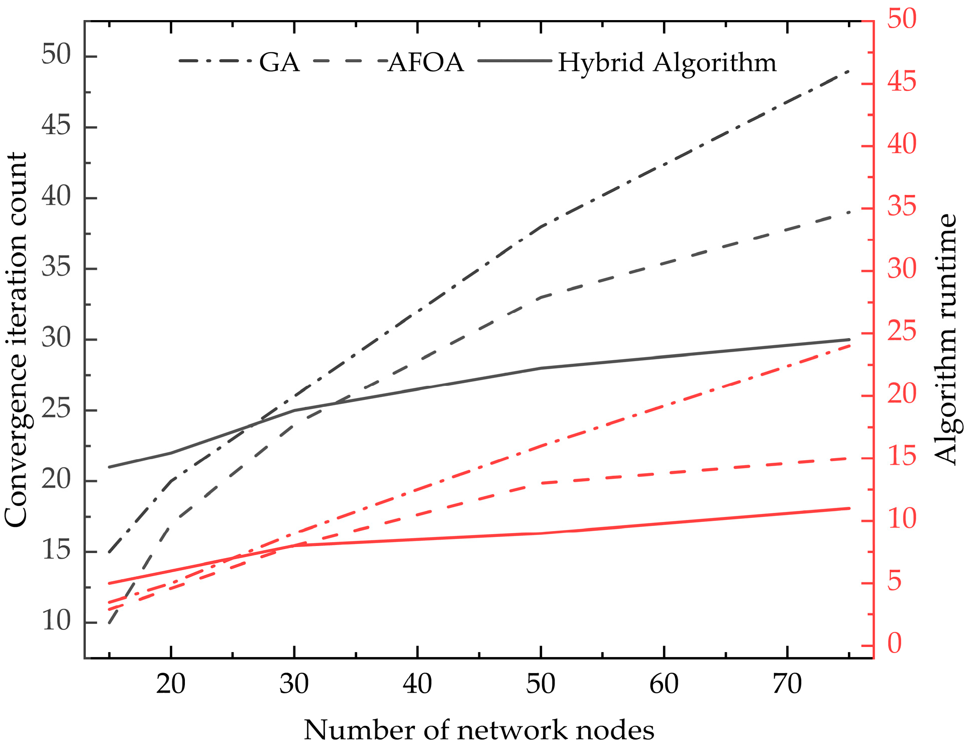
In terms of algorithm design: A fusion of GA and AFO is adopted. GA is utilized to generate the initial population, and then AFO is employed for iterative calculations. This approach avoids both the tendency of GA to fall into local optima and the slow iteration speed of AFO.

(3)

In terms of decision-making methods: A four-objective optimization model is constructed to minimize generalized transportation costs, transportation time, carbon emissions, and risks. By designing a fuzzy evaluation matrix, the demand preference information of multimodal transportation participants is quantified, thereby achieving a deep integration of transportation scheme formulation with user preferences.

3. Problem Description and Model Construction

A multimodal transportation network differs from a single-mode transportation network in that it is an aggregation of multiple transportation modes. The presence of these diverse modes inevitably leads to transfers, which in turn give rise to trans-shipment costs. This is precisely what fundamentally distinguishes the multimodal transportation routing problem from the simple “shortest route” problem. Drawing on the unique characteristics of multimodal transportation, this text defines a specific type of multimodal transportation network and establishes a corresponding route optimization model based on the features of various transportation modes.

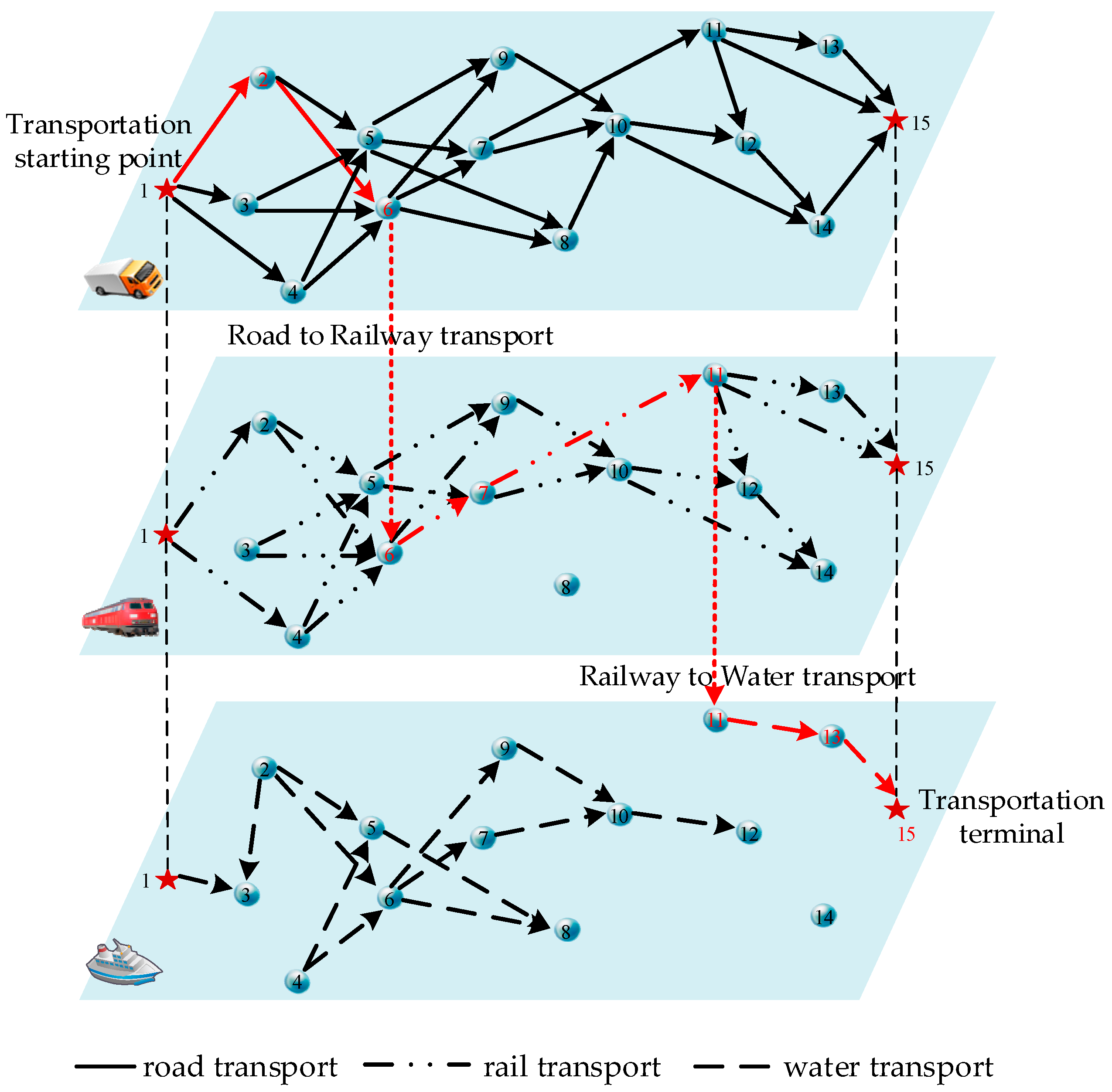
3.1. Problem Description

The multimodal transportation network is defined as shown in Figure 1, where $V$ represents the set of nodes, $E$ represents the set of arcs, and $D$ represents the set of transportation modes. The multimodal transportation operator will plan a reasonable route to transport goods from the origin to the destination, taking into account factors such as cost, time, carbon emissions, and risk. The transportation route will pass through multiple intermediate nodes in the network and may involve mode transfers at some nodes.

3.2. Assumptions

Assumption 1.

Cargo cannot be split for transportation at any node.

Assumption 2.

Cargo can only undergo a maximum of one transportation mode transfer at intermediate nodes.

Assumption 3.

After completing the transfer and unloading operations, the cargo will be transported to the subsequent node according to the nearest departure time of the selected transportation mode.

Assumption 4.

Given the complexity involved in formulating flight schedules, we assume that air transportation is not an available option, and the alternative transportation modes to choose from are highway, railway, and waterway transportation.

3.3. Parameter Description

The set of nodes ($V$): $\left\{o,\cdots ,i,j,\cdots d\right\}\in V$, where o and d represent the origin and destination of the transportation, respectively.

The set of arcs ($E$): $(i,j)\in E$, where (i, j) represents an arc in the intermodal transportation network.

The set of transportation modes ($D$): $(m,n)\in D$, where m, n represent different transportation modes.

$U_i$: The set of backward neighboring nodes of node $i$.

$q$: Cargo volume.

$(i,j)$: Directed arc from node i to node j in the intermodal transportation network.

$t_{ij}^m$: Transportation time of mode m on the directed arc (i, j).

$Q_{ij}^m$: Maximum transportation capacity of mode m on the directed arc (i, j).

$d_{ij}^m$: Transportation distance of mode m on the directed arc (i, j).

$v_{ij}^m$: Transportation speed of mode m on the directed arc (i, j).

$c_{ij}^m$: Unit transportation cost of mode m on the directed arc (i, j).

$c_i$: Waiting cost of cargo at node i.

$e_{ij}^m$: Unit distance carbon emission of mode m on the directed arc (i, j).

$r_{ij}^m$: Transportation risk of mode m on the directed arc (i, j).

$t_i^{mn}$: Transfer time at node i from mode m to mode n.

$c_i^{mn}$: Transfer cost at node i from mode m to mode n.

$Q_i^{mn}$: Transfer capacity at node i from mode m to mode n.

$e_i^{mn}$: Unit carbon emission coefficient for trans-shipment at node i from mode m to mode n.

$r_i^{mn}$: Transfer risk at node i for trans-shipment from mode m to mode n.

$T_i^{\mathrm{A}}$: Departure time from node i using mode m.

${\delta }_j$: Waiting time at node j before departure.

$T_j^{\mathrm{L}}$: Departure time from node.

$T_j^{\mathrm{A}}$: Arrival time at node j from node i using mode m.

$T_{end}$: Arrival time at the destination.

$\omega$: The set of weights for various indicators.

Soft time window ($[T^e,T^l]$): the customer’s desired earliest and latest arrival times for the cargo.

Hard time window ($[ET,LT]$): the customer’s tolerable earliest and latest arrival times for the cargo.

The following are the variables in the model, while the parameters in the model are as previously described:

$x_{ij}^m$: If mode m is selected to transport cargo on the directed arc(i, j), then $x_{ij}^m=1$; otherwise, $x_{ij}^m=0$.

$y_i^{mn}$: If the transportation mode is transferred from m to n at node i, then $y_i^{mn}=1$; otherwise, $y_i^{mn}=0$.

3.4. Model Construction

Considering that railway transportation is influenced by train scheduling, there will be waiting time associated with transportation mode transfers involving railway transportation. When cargo is transferred at a certain node, the total transfer time is determined, as illustrated in Figure 2. If the subsequent transportation mode is railway transportation, there will be a waiting time $\Delta t_{34}$. Based on this, a multi-objective route optimization model is established, as shown in Equations (1)–(18).

Equations (1)–(5) represent the objective functions.

Equation (1) aims to minimize the total cost, total time, total carbon emissions, and total risk.

$$\mathit{min}\left\{C,T,E,R\right\}$$

(1)

Equation (2) represents the total cost, which includes transportation costs, transfer costs, and waiting costs.

$$C={\displaystyle \sum _{i\in V}{\displaystyle \sum _{j\in V}{\displaystyle \sum _{m\in D}q{c}_{ij}^m}}}{x}_{ij}^m+{\displaystyle \sum _{i\in V}{\displaystyle \sum _{m\in D}{\displaystyle \sum _{n\in D}{y}_i^{mn}q(c_i^{mn}+c_i\mathit{max}(T_j^{\mathrm{L}}-{\delta }_j,0)}}})$$

(2)

Equation (3) represents the total time, which includes transportation time, loading/unloading and marshalling time, and waiting time.

$$T={\displaystyle \sum _{i\in V}{\displaystyle \sum _{j\in V}{\displaystyle \sum _{m\in D}{x}_{ij}^m}}}{\displaystyle \frac{d_{ij}^m}{v_{ij}^m}}+{\displaystyle \sum _{i\in V}{\displaystyle \sum _{j\in V}{\displaystyle \sum _{m\in D}{\displaystyle \sum _{n\in D}{y}_i^{mn}(}}}q{t}_i^{mn}+\mathit{max}(T_j^{\mathrm{L}}-{\delta }_j,0)})$$

(3)

Equation (4) represents the total carbon emissions, which include transportation carbon emissions and transfer carbon emissions.

$$E={\displaystyle \sum _{i\in V}{\displaystyle \sum _{j\in V}{\displaystyle \sum _{m\in D}q{e}_{ij}^m}}}{d}_{ij}^m{x}_{ij}^m+{\displaystyle \sum _{i\in V}{\displaystyle \sum _{m\in D}{\displaystyle \sum _{n\in D}q{e}_i^{mn}}}}{y}_i^{mn}$$

(4)

Equation (5) represents the total risk, which includes transportation risk and transfer risk.

$$R={\displaystyle \sum _{i\in V}{\displaystyle \sum _{j\in V}{\displaystyle \sum _{m\in D}{r}_{ij}^m{x}_{ij}^m}}}+{\displaystyle \sum _{i\in V}{\displaystyle \sum _{m\in D}{\displaystyle \sum _{n\in D}{r}_i^{mn}{y}_i^{mn}}}}$$

(5)

Equations (6)–(17) represent the constraints.

Equation (6) indicates the time when the cargo departs from node i and arrives at the next node j via transportation mode m.

$$T_j^{\mathrm{A}}=T_i^{\mathrm{L}}+t_{ij}^m,i,j\in V;m\in D$$

(6)

Equation (7) represents the moment when the transfer, loading, and unloading operations are completed.

$${\delta }_j=T_j^{\mathrm{A}}+t_j^{mn},j\in V;m,n\in D$$

(7)

In Equation (8), $\omega ({\delta }_j,n)$ represents the nearest departure time for adopting transportation mode n in the next stage of the journey at moment ${\delta }_j$.

$$T_j^{\mathrm{L}}=\omega ({\delta }_j,n),j\in V;n\in D$$

(8)

Equation (9) states that the total travel time for the cargo to reach the destination should not exceed the maximum time allowed by the consignee.

$$T_d^{\mathrm{A}}⩽T_{\mathrm{END}}$$

(9)

Equation (10) is the flow balance constraint.

$$\sum _{j\in V}\sum _{m\in D}{x}_{ij}^m-\sum _{j\in V}\sum _{m\in D}{x}_{ji}^m=\left\{\begin{array}{l}-1,i\in o\hfill \\ 0,i\in V\backslash \{o,d\}\hfill \\ 1,i\in d\hfill \end{array}\right.$$

(10)

Equation (11) ensures the continuity of transportation.

$$\begin{gathered} \mathrm{If} y_i^{mn}=1, \mathrm{then} x_{ki}^m=1, x_{ij}^n=1\mathrm{and}\sum _{i,j\in V}\sum _{l\in D}{x}_{ij}^l=1 , \\ l,m,n\in D;k,i,j\in V;i\in U_k,j\in U_i \end{gathered}$$

(11)

Equation (12) indicates that, at most, one transportation mode can be selected between adjacent nodes.

$$\sum _{j\in V}\sum _{m\in D}{x}_{ij}^m\le 1,i\in V$$

(12)

Equation (13) states that the cargo can be transferred, at most, once at any node.

$$\sum _{m,n\in D}{y}_i^{mn}\le 1,i\in V$$

(13)

Equation (14) indicates that the cargo volume cannot exceed the transportation capacity of the selected transportation mode between two nodes.

$$q{x}_{ij}^m\le Q_{ij}^m,m\in D;i,j\in V$$

(14)

Equation (15) states that the cargo volume cannot exceed the transfer capacity of the transfer node.

$$q{y}_i^{mn}\le Q_i^{mn},m,n\in D;i\in V$$

(15)

Equation (16) indicates that no transfer occurs between the same transportation modes.

$$y_i^{mm}=0,m\in D;i\in V$$

(16)

Equation (17) states that no transfer can occur at the origin and destination of the cargo.

$$x_{ii}^m=0,y_i^{mn}=0,i\in V\left\{o,d\right\};m,n\in D$$

(17)

In order to balance various decision-making indicators and reach a unified decision in the end, we assigned weights to each indicator and transformed the objective function (1) into the form shown in Equation (18).

$$\mathit{min}Z=\mathit{min}\left({\omega }_{1}C+{\omega }_{2}T+{\omega }_{3}E+{\omega }_{4}R\right),{\omega }_1,{\omega }_2,{\omega }_2,{\omega }_2\in \omega$$

(18)

4. Methodology

The multimodal transportation route optimization problem is a typical combinatorial optimization problem. Based on the characteristics of the problem, initially, the GA is employed to obtain several promising solutions, which serve as the initial population for the AFO. This approach reduces the number of convergence iterations in the early stages of AFO. Subsequently, through the application of the movement strategy of AFO, the population is guided to search for optimal solutions in the solution space, further enhancing the solution accuracy of the algorithm. The flowchart of the GA-AFO hybrid algorithm is depicted in Figure 3.

4.1. Genetic Algorithm

In the GA, the reciprocal of the objective function value is employed as the fitness function, and the tournament selection method is utilized for the selection operation. The encoding, decoding, and genetic operations are described as follows.

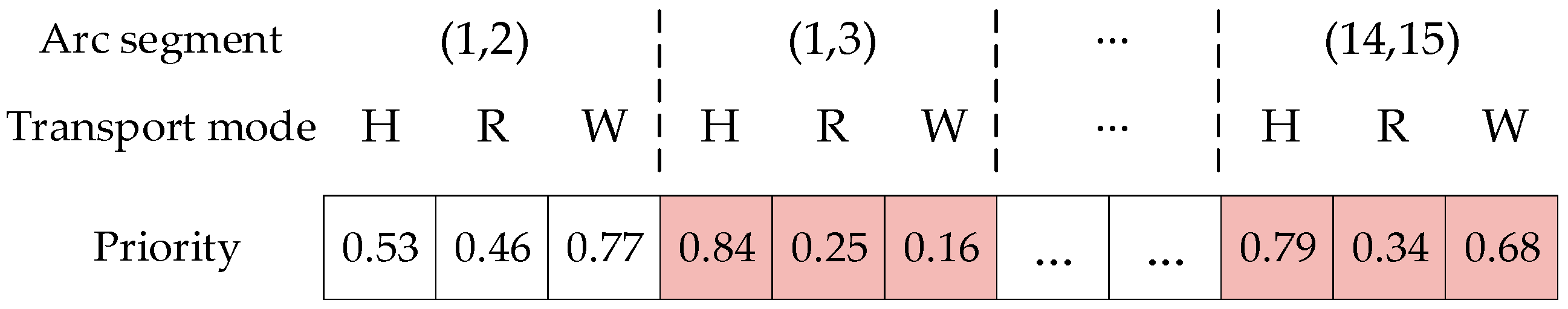
4.1.1. Encoding and Decoding

A node connectivity database is established based on the network topology to characterize the interrelationships between nodes.

Subsequently, for each arc segment in the network, we randomly assign a unique real-value priority to the three transportation modes: highway, railway, and waterway. These priority values are sequentially stored in the chromosome vector, thereby completing the construction of a single chromosome. By repeating this process for the predefined number of chromosomes, we can construct the entire population of chromosomes.

Specifically, under this encoding scheme, each chromosome is represented as a vector of length N × 3, where N represents the total number of arc segments in the network. The structure of this vector is as follows: for each arc segment (there are N in total), we sequentially store the priority values for the highway transportation mode, the railway transportation mode, and the waterway transportation mode. Consequently, the overall length of the vector is the number of arc segments N multiplied by the number of transportation modes 3, which equals N × 3.

This encoding method ensures that each chromosome is of equal length and contains the priority information for all arc segments and all transportation modes within the network, thereby providing a solid foundation for subsequent genetic operations, such as selection, crossover, and mutation. The encoding scheme is illustrated in Figure 4, where H, R, and W denote highway, railway, and waterway transportation modes, respectively.

The decoding process is conducted through the following steps:

Step 1: Starting from the origin node, identify the set of reachable nodes as the candidate node set.

Step 2: Select the transportation mode with the highest priority among the candidate nodes corresponding to the current node. Record the selected node and the adopted transportation mode.

Step 3: Repeat the above operations until the destination node is reached, and output the combined path and transportation mode scheme.

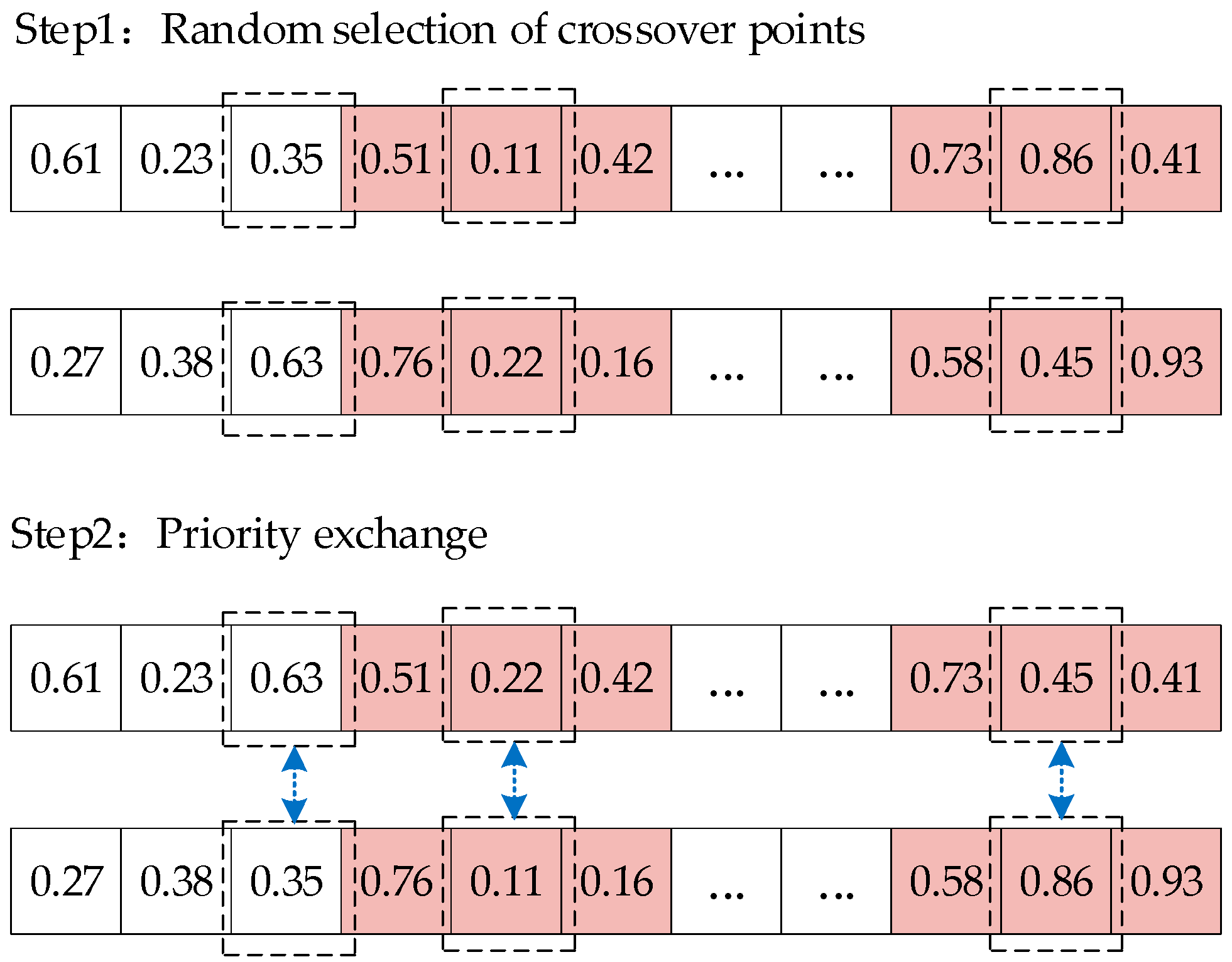
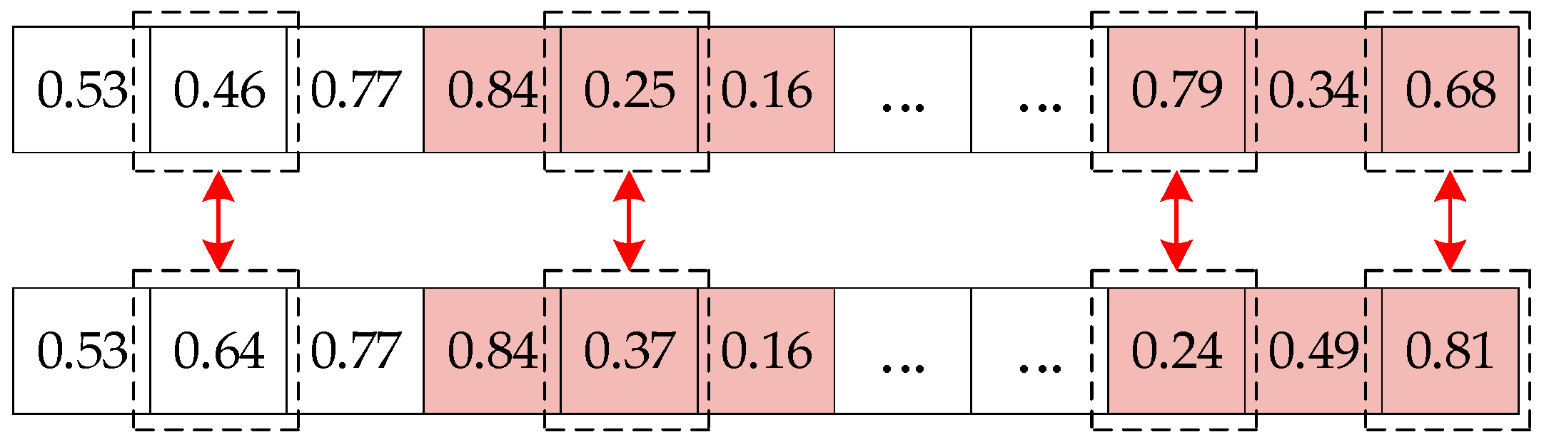
4.1.2. Crossover and Mutation

Multi-point crossover is applied to chromosomes. A certain number of gene loci are randomly selected, and the genes at these loci are exchanged between two parent chromosomes. To prevent excessive crossover from disrupting the structure of high-quality genes, the upper limit of the number of selected genes is set to 50% of the chromosome length. The crossover process is depicted in Figure 5.

Uniform random mutation is performed on chromosomes. A certain number of gene loci are randomly selected, and the genes at these loci are replaced with randomly generated priority values. To avoid excessive mutation from undermining the structure of high-quality genes, the upper limit of the number of mutated genes is set to 30% of the chromosome length. The mutation process is illustrated in Figure 6.

4.2. Hybrid Algorithm

The AFO is a metaheuristic algorithm proposed by Yang [31] in 2021, inspired by the phenomenon of emperor penguins huddling together for warmth in winter. The individual with the highest temperature at the center of the emperor penguin group is considered the optimal individual, while other peripheral individuals move towards the center through several movement strategies.

The priority-based chromosome encoding scheme designed in this paper serves as the foundation for ensuring the effective integration of the GA and the AFO. Each chromosome is represented as a randomly permuted sequence of N × 3 numbers, which not only guarantees that all chromosomes are feasible solutions but also ensures a seamless transition to the AFO algorithm. This is because the structural design of each chromosome aligns precisely with the individual structure of the penguin entities within the AFO population.

When searching for a suitable position, emperor penguins need to perceive changes in temperature, consider the positions of other penguins, move towards the center of the population, and consult their own memory to reduce energy loss. These five modes combine to evolve into three movement strategies for variables.

The first movement strategy is a local search strategy based on gradient estimation. An emperor penguin individual’s perception of the direction of temperature change corresponds to its judgment of the temperature gradient direction. The temperature gradient is a physical quantity that describes the direction and rate of the fastest temperature change in a specific regional environment. In a continuous temperature field, the direction of the maximum temperature change rate at a certain point is in the normal direction of the isotherms, which requires derivation and solution of the target model. However, the multi-modal transportation route optimization problem is a 0–1 integer programming problem with discrete characteristics, making it impossible to calculate its derivative. Therefore, Movement Strategy 1 in the traditional AFO is replaced by a mutation strategy as shown in Figure 7, where the probabilities of selecting 0 and 1 are 0.4 and 0.6, respectively. $X_i\left(a\right)$ not only can inherit some characteristics from $X_i\left(a-1\right)$ but also can generate new characteristics after random mutation operations. The similarity between $X_i\left(a\right)$ and $X_i\left(a-1\right)$ is small, indicating that the mutation operation helps enhance diversity and maintain the genetic nature of the algorithm.

The second movement strategy involves, when penguins gather together for warmth, the position adjustment of an individual emperor penguin considering the positions of surrounding penguins. Within the penguin population, the best positions remembered by two randomly selected emperor penguins are $X{m}_{p_1}\left(a\right)$ and $X{m}_{p_2}\left(a\right)$, with their corresponding objective function values being $Y{m}_{p_1}\left(a\right)$ and $Y{m}_{p_2}\left(a\right)$, respectively. $\gamma$ is the influence coefficient of the positions of other emperor penguins on its displacement. $P_1$ is a random number matrix uniformly distributed between 0 and 1, with the same dimensions as $X_i\left(a\right)$. The formulas for calculating $X_i\left(a\right)$ and $\gamma$ are given by Equations (19) and (20), respectively.

$$X_i(a)=X_i(a-1)+P_1\gamma (X{m}_{p_1}(a-1)-X{m}_{p_2}(a-1))(-sgn(Y{m}_{p_1}(a-1)-Y{m}_{p_2}(a-1)))$$

(19)

$$\gamma =arc tanh(1-{\displaystyle \frac{a}{\max gen}})$$

(20)

The third movement strategy is a combination that comprehensively considers the penguin’s own position, the central position of the population, and energy loss. $X{m}_i\left(a\right)$ represents the position corresponding to the best temperature $Y{m}_i\left(a\right)$ remembered by the emperor penguin at time t. $P_2$ is a random number matrix that follows a standard normal distribution, with dimensions equal to $X_i\left(a\right)$. $\delta$ is the memory influence factor, $Xc\left(a\right)$ is the central position of the population, $\epsilon$ is the influence factor of the population center. E is the displacement influence coefficient at the previous moment. $A_i\left(a-1\right)$ is the displacement at the previous moment, and ${\lambda }_1, {\lambda }_2, {\lambda }_3$ are weight coefficients. The formulas for calculating the penguin’s displacement and its position at time t are given by Equations (20) and (21), respectively.

$$A_i(a)={\lambda }_1{P}_2\beta (X{m}_i(a-1)-X_i(a-1))+{\lambda }_2\delta (Xc(a-1)-X_i(a-1))+{\lambda }_3\epsilon A_i(a-1)$$

(21)

$$X_i(a)=X_i(a-1)+A_i(a)$$

(22)

To prevent the algorithm from falling into a local optimum, this paper introduces a catastrophe operation. During the search process, if the algorithm is deemed to be converging prematurely, a catastrophic strategy is employed: except for one penguin located at the center of the population, the current positions of all other penguins are regenerated, and their memories are cleared. The criterion for judging premature convergence of the algorithm is that the temperature change at the center of the penguin population before and after the search within the current iteration cycle is less than 1%, as shown in Equation (23):

$$count=count+1, 0.99Y_g^{a-1}\le Y_g^a$$

(23)

When the algorithm satisfies the above criterion consecutively for L times (count > L), it is considered to be in a state of premature convergence, and the catastrophe strategy is adopted.

4.3. Multi-Attribute Decision Making

The decision-making indicators for transportation schemes encompass cost, carbon emissions, time, and risk. To reconcile the tension between personal preferences and objective weights, an uncertain multi-attribute decision-making method [32] is employed. This method harmonizes users’ subjective preferences for indicators with their objective weights, leveraging the complementary strengths of both, to produce a more scientifically sound and rational decision-making outcome. The steps for scheme decision making are as follows:

Step 1: List the decision indicators of all alternative schemes in a matrix form $A=(a_{ij}),i\in N,j\in M$, where $N$ denotes the number of schemes and $M$ represents the number of evaluation criteria.

Step 2: To eliminate dimensional differences, normalize the matrix by Equation (24).

$$R=(r_{ij})={\displaystyle \frac{\underset{i}{\min }\left(a_{ij}\right)}{a_{ij}}},i\in N,j\in M$$

(24)

Step 3: To unify decision-making information, incorporate the objective weights $W=({\omega }_1,{\omega }_2,\cdots ,{\omega }_k)$ into the normalized matrix $R$, and construct the objective complementary judgment matrix $\overline{B}={({\overline{b}}_{ij})}_{i\times i}$, where ${\overline{b}}_{ij}={\displaystyle \frac{1}{2}}\left[1+{\displaystyle \sum _{k=1}^k{r}_{ik}{\omega }_k}-{\displaystyle \sum _{k=1}^k{r}_{jk}{\omega }_k}\right],i,j\in N$.

Step 4: Based on decision makers’ subjective preferences, construct the subjective complementary judgment matrix $B={(b_{ij})}_{i\times i}$ using the 0.1–0.9 complementary scale, where $b_{ij}+b_{ji}={\overline{b}}_{ij}+{\overline{b}}_{ji}=1$, $b_{ii}={\overline{b}}_{ii}=0.5$, $b_{ii}\ge 0,{\overline{b}}_{ii}\ge 0,i,j\in N$.

Step 5: Integrate subjective and objective weights by defining the deviation function $f_{ij}=b_{ij}-{\overline{b}}_{ij},i,j\in N$ and then formulate the single-objective optimization model by Equation (25).

$$\left\{\begin{array}{l}\min F(\omega )={\displaystyle \sum _{i=1}^n{\displaystyle \sum _{j=1}^n{f_{ij}}^2}}\hfill \\ s.t.{\omega }_j\ge 0,j\in M,{\displaystyle \sum _{j=1}^m{\omega }_j=1}\hfill \end{array}\right.$$

(25)

Step 6: Solve the above optimization problem to obtain the integrated weights $\omega =({\omega }_1,{\omega }_2,\cdots ,{\omega }_k)$, calculate the comprehensive attribute value of each scheme using $z_i(\omega )={\displaystyle \sum _{j=1}^m{r}_{ij}{\omega }_j},i\in N,j\in M$, and rank the schemes to determine the optimal alternative.

5. Case Study

To verify the validity of the model and the applicability of the algorithm, this paper constructs a multimodal transportation network as shown in Figure 1. Based on this network, we set specific configurations and key parameters to simulate the complexity and diversity of real-world transportation scenarios. Subsequently, we employed the methods mentioned above to first solve the case, and on the basis of the solution, discussed the final decision-making scheme.

5.1. Case Description

The network involves 15 nodes, 28 arcs, and three transportation modes, highway, railway, and waterway, with a transportation demand of 150 tons. We adopt average speeds, where the average speeds for highway, railway, and waterway transportation are 75 km/h, 60 km/h, and 30 km/h, respectively. Additional attributes of the intermodal transportation network are detailed in

Table 1. Transfer costs/times/carbon emissions at the nodes.

	Highway	Railway	Waterway
Highway	0	3.09/1/1.56	5.23/1/6
Railway	3.09/1/1.56	0	26.62/2/3.12
Waterway	5.23/1/6	26.62/2/3.12	0

The units for the data in the table are CNY/t, h, and kg/t.

,

Table 2. Characteristics and values of each transportation mode.

Transportation Mode	Data Category	Value
Highway	Transportation cost (CNY (t/km)−1)	0.3
	Carbon emission factor (kg (t/km)−1)	0.796
Railway	Transportation cost (CNY (t/km)−1)	0.2
	Carbon emission factor (kg (t/km)−1)	0.028
Waterway	Transportation cost (CNY (t/km)−1)	0.1
	Carbon emission factor (kg (t/km)−1)	0.04

and

Table 3. Transportation distances and capacities for different transportation modes on each arc.

Transportation Arc Segment	Highway			Railway			Waterway
	Distance/km	Capacity/t	Risk	Distance/km	Capacity/t	Risk	Distance/km	Capacity/t	Risk
(1, 2)	400	160	20	312	180	12	—	—	—
(1, 3)	350	190	18	—	—	—	650	175	10
(1, 4)	435	168	10	424	190	8	—	—	—
(2, 3)	700	110	10	—	—	—	550	210	15
(2, 5)	318	210	20	335	220	20	463	190	20
(2, 6)	428	168	25	390	190	20	453	185	12
(3, 5)	285	180	15	379	195	25	—	—	—
(3, 6)	306	100	14	337	110	18	—	—	—
(4, 5)	264	180	13	275	230	14	342	210	18
(4, 6)	273	170	10	289	140	10	352	200	11
(5, 7)	250	215	4	369	228	8	—	—	—
(5, 8)	700	200	9	—	—	—	650	180	10
(5, 9)	509	180	5	458	195	6	—	—	—
(6, 7)	441	230	6	851	220	16	420	230	8
(6, 8)	345	400	12	—	—	—	392	390	12
(6, 9)	513	220	10	231	190	10	496	198	5
(7, 10)	400	180	8	468	220	8	460	215	6
(7, 11)	608	180	18	655	195	14	—	—	—
(8, 10)	124	215	4	—	—	—	—	—	—
(9, 10)	100	200	4	163	220	5	158	180	4
(10, 12)	292	220	15	399	230	16	—	—	—
(10, 14)	523	180	8	485	228	8	—	—	—
(11, 12)	290	170	14	399	140	15	—	—	—
(11, 13)	284	150	10	266	195	12	317	182	16
(11, 15)	600	200	8	482	210	6	—	—	—
(12, 14)	369	220	19	—	—	—	—	—	—
(13, 15)	141	200	4	274	220	5	119	180	5
(14, 15)	379	180	10	—	—	—	—	—	—

“—” indicates that this arc segment does not have this mode of transportation.

. Table 1 presents the intermodal transfer costs among different transportation modes, Table 2 provides the unit costs and unit carbon emissions associated with each mode, and Table 3 lists the segment lengths, capacities, and risk metrics for each route section.

5.2. Case Solution

The GA-AFO hybrid algorithm was implemented using MATLAB 2023a and evaluated on a Windows 10 system equipped with a 2.40 GHz processor and 8.00 GB of RAM. Key parameters were configured as follows:

Population size: 50 individuals;

GA iterations (generations): 20 (evolutionary cycles of the genetic algorithm);

AFO iterations (outer loop): 100 (outer optimization loop of the AFO algorithm);

Crossover probability: 0.7;

Mutation probability: 0.1.

This configuration ensures a balance between exploration (via 20 GA generations) and exploitation (via 100 AFO outer-loop iterations), with the GA refining the population structure and the AFO component fine-tuning individual solutions.

The GA-AFO algorithm, as well as the GA and AFO algorithms, each were executed 20 times independently. The best-performing run from each algorithm was selected for comparison, and the results are illustrated in Figure 8. It can be observed that all three algorithms are capable of obtaining the optimal solution. To further validate the efficiency of these algorithms, we tested them on networks with varying numbers of nodes. All three algorithms were able to converge to the same optimal solution, and their iterative convergence processes are depicted in Figure 9. In the figure, the horizontal axis represents the number of nodes in the network, while the vertical axes denote the number of iterations and the iteration time required for the algorithms to converge, respectively. It can be seen that when the network is relatively small, the hybrid GA-AFO algorithm, due to the initial iterations of GA in its early stages, requires slightly more iterations to converge compared to the standalone GA and AFO algorithms. However, as the complexity of the network gradually increases, the number of iterations and the iteration time for both the GA and AFO algorithms rise sharply, whereas those for the hybrid algorithm increase at a much slower pace, maintaining a relatively stable state. This demonstrates the hybrid algorithm’s excellent accuracy and efficiency.

Table 4. Transportation schemes.

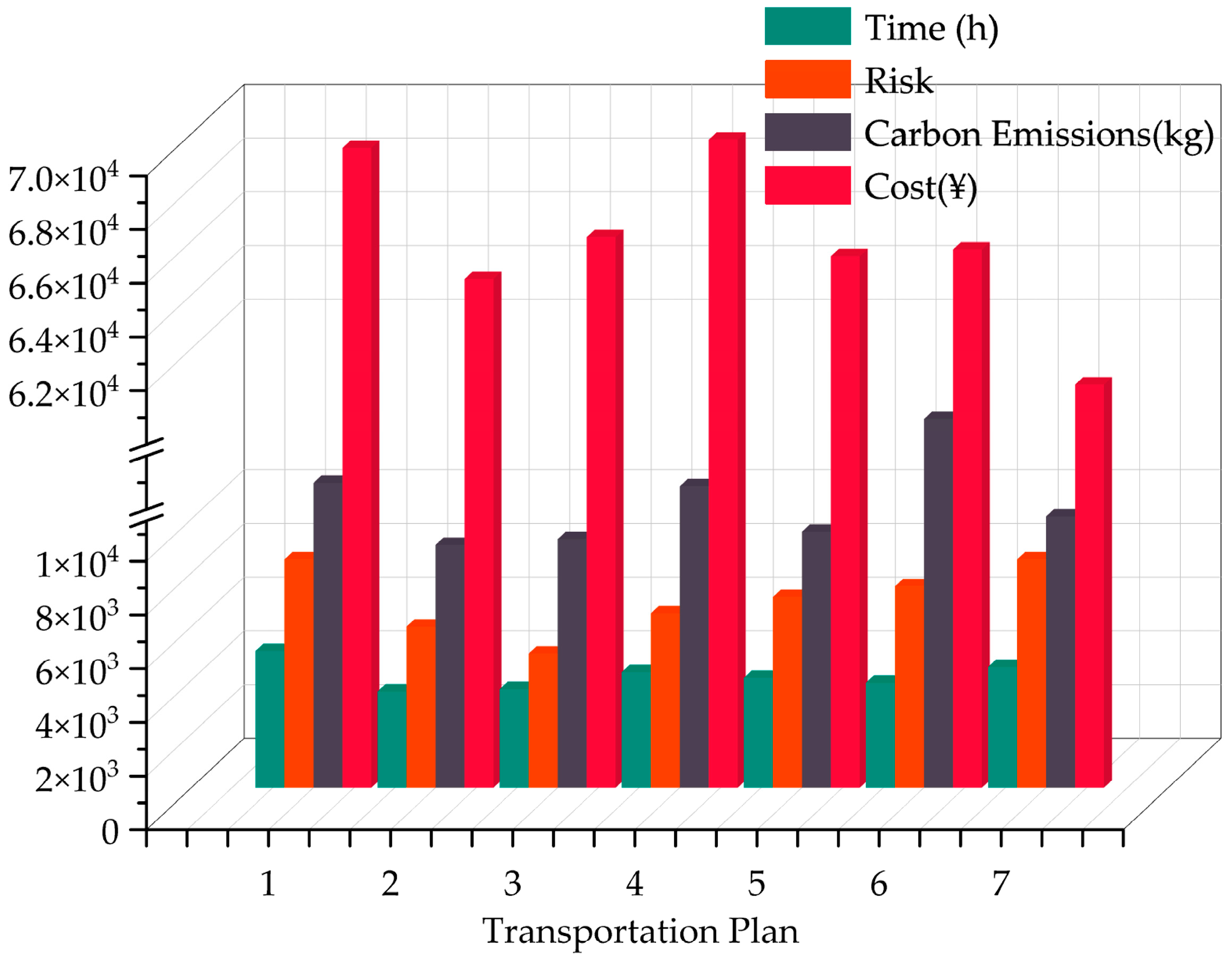
Scheme	Transportation Path	Transportation Mode	Cost/CNY	Carbon Emission/kg	Time/h	Risk
1	1-2-5-7-11-15	Railway-Waterway-Railway-Railway-Railway	69,471	11,350	50.95	85
2	1-2-5-7-11-15	Railway-Railway-Railway-Railway-Railway	64,590	9042.6	35.89	60
3	1-4-5-7-11-15	Railway-Railway-Railway-Railway-Railway	66,150	9261	36.75	50
4	1-4-6-7-11-15	Railway-Railway-Waterway-Railway-Railway	69,786	11,226	53.04	65
5	1-4-5-7-11-13-15	Railway-Railway-Railway-Railway-Railway-Waterway	65,448	9535.8	40.89	71
6	1-2-5-7-11-15	Railway-Railway-Highway-Railway-Railway	65,697	37,811	39.1	75
7	1-2-5-7-11-13-15	Railway-Railway-Railway-Railway-Waterway-Waterway	60,663	10,102	44.96	85

presents the optimized transportation schemes and their corresponding performance indicators. The disparities among these schemes in terms of transportation cost, carbon emissions, travel duration, and risk exposure are visually illustrated in Figure 10. It is evident that each scheme exhibits distinct strengths and weaknesses. For instance, Scheme 7 achieves the lowest transportation cost, while maintaining moderate levels of carbon emissions and travel time, yet it incurs the highest transportation risk. In contrast, Scheme 2 leads in carbon efficiency and shortest delivery time, with its cost and risk profiles ranking second among all options. Meanwhile, Scheme 3 prioritizes risk minimization, while its carbon emissions and travel time rank second, and its cost efficiency places it fifth. Given that different stakeholders exhibit heterogeneous preferences for these performance metrics, it becomes imperative to apply the multi-attribute decision-making methodology to facilitate a structured evaluation and selection process.

5.3. Decision Result Discussion

Building upon the aforementioned research, we further delve into the decision-making strategies of different participants with varying preferences. Whether they are managers, carriers, or shippers, we assume that rational decision makers, in the absence of other influencing factors, consistently gravitate towards selecting the transportation option with the lowest cost. However, the other three factors—carbon emissions, transportation risk, and transit time—respectively represent the perspectives of managers, carriers, and shippers. Managers aim to accomplish transportation tasks with the lowest possible carbon emissions, carriers seek to minimize risks encountered during transit, and shippers desire their goods to be delivered as swiftly as possible. To more clearly analyze these three categories of preferences, we have magnified them by selecting three specific transportation scenarios for testing. Scenario 1 mandates strict adherence to carbon emission policies. Scenario 2 involves the transportation of hazardous goods, where the management and control of transportation risks take precedence. Scenario 3 pertains to the transportation of perishable goods, with the primary focus being the control of transit time, and its time window is set within the range of [36,39] hours.

$B(\mathrm{Scenario} 1)$, $B(\mathrm{Scenario} 2)$, $B(\mathrm{Scenario} 3)$ each provided their subjective complementary judgment matrices under different scenarios, and the decision-making results under these varying scenarios are presented in

Table 5. Decision-making results under varying scenarios.

Scenarios	Scenario 1	Scenario 2	Scenario 3
$W$	${\omega }_1$ = 0.2187	${\omega }_1$ = 0.2918	${\omega }_1$ = 0.7246
	${\omega }_2$ = 0.4692	${\omega }_2$ = 0.1275	${\omega }_2$ = 0.0145
	${\omega }_3$ = 0.2025	${\omega }_3$ = 0.2307	${\omega }_3$ = 0.1140
	${\omega }_4$ = 0.1096	${\omega }_4$ = 0.3500	${\omega }_4$ = 0.0469
$Z$	$z\left(x_1\right)$ = 0.7717	$z\left(x_1\right)$ = 0.7248	$z\left(x_1\right)$ = 0.7522
	$z\left(x_2\right)$ = 0.9684	$z\left(x_2\right)$ = 0.9239	$z\left(x_2\right)$ = 0.8481
	$z\left(x_3\right)$ = 0.9661	$z\left(x_3\right)$ = 0.9674	$z\left(x_3\right)$ = 0.8369
	$z\left(x_4\right)$ = 0.7894	$z\left(x_4\right)$ = 0.7817	$z\left(x_4\right)$ = 0.7548
	$z\left(x_5\right)$ = 0.9026	$z\left(x_5\right)$ = 0.8403	$z\left(x_5\right)$ = 0.8185
	$z\left(x_6\right)$ = 0.5731	$z\left(x_6\right)$ = 0.7450	$z\left(x_6\right)$ = 0.8085
	$z\left(x_7\right)$ = 0.8648	$z\left(x_7\right)$ = 0.7960	$z\left(x_7\right)$ = 0.8562
Scheme ranking	$x_2,x_3,x_5,x_7,x_4,x_1,x_6$	$x_3,x_2,x_5,x_7,x_4,x_6,x_1$	$x_7,x_2,x_3,x_5,x_6,x_4,x_1$

.

$$B(\mathrm{Scenario} 1)=\left|\begin{array}{ccccccc}0.5& 0.1& 0.2& 0.3& 0.2& 0.3& 0.1\\ 0.9& 0.5& 0.6& 0.9& 0.6& 0.6& 0.1\\ 0.8& 0.4& 0.5& 0.9& 0.3& 0.3& 0.1\\ 0.7& 0.1& 0.1& 0.5& 0.2& 0.2& 0.1\\ 0.8& 0.4& 0.7& 0.8& 0.5& 0.5& 0.3\\ 0.7& 0.4& 0.7& 0.8& 0.5& 0.5& 0.3\\ 0.9& 0.9& 0.9& 0.9& 0.7& 0.7& 0.5\end{array}\right|$$

$$B(\mathrm{Scenario} 2)=\left|\begin{array}{ccccccc}0.5& 0.1& 0.1& 0.2& 0.3& 0.3& 0.5\\ 0.9& 0.5& 0.3& 0.7& 0.8& 0.8& 0.9\\ 0.9& 0.7& 0.5& 0.8& 0.9& 0.9& 0.9\\ 0.8& 0.3& 0.2& 0.5& 0.7& 0.8& 0.9\\ 0.7& 0.2& 0.1& 0.3& 0.5& 0.7& 0.9\\ 0.7& 0.2& 0.1& 0.2& 0.3& 0.5& 0.8\\ 0.5& 0.1& 0.1& 0.1& 0.1& 0.2& 0.5\end{array}\right|$$

$$B(\mathrm{Scenario} 3)=\left|\begin{array}{ccccccc}0.5& 0.1& 0.1& 0.7& 0.2& 0.2& 0.3\\ 0.9& 0.5& 0.5& 0.9& 0.7& 0.7& 0.8\\ 0.9& 0.5& 0.5& 0.9& 0.8& 0.7& 0.8\\ 0.3& 0.1& 0.1& 0.5& 0.3& 0.3& 0.6\\ 0.8& 0.3& 0.2& 0.7& 0.5& 0.4& 0.8\\ 0.8& 0.3& 0.3& 0.7& 0.6& 0.5& 0.8\\ 0.7& 0.2& 0.2& 0.4& 0.2& 0.2& 0.5\end{array}\right|$$

As evident from the aforementioned schemes, different preferences of decision makers lead to distinct optimal schemes. From the perspective of carbon emission control, Scheme 2 boasts the lowest carbon emissions and is ultimately selected. When considering risk control, Scheme 3 presents the least risk and is chosen accordingly. However, if time control is the priority, although Scheme 2 has the shortest duration, Scheme 7 is ultimately selected because it has the lowest cost among all the options. This illustrates that, within an acceptable range, it is also acceptable to appropriately extend transportation time to reduce transportation costs. It further demonstrates that the subjective complementary judgment matrices provided by decision makers can influence the scheme selection to a certain extent, but they are not the sole determinant.

On the whole, regardless of the decision makers’ preferences, Scheme 2 and Scheme 3 consistently emerge as the top recommended options. These two schemes indeed exhibit relatively low levels of carbon emissions, risk, and duration, with transportation costs falling within an acceptable mid-range. Additionally, neither of these schemes involves a change in transportation mode, which often makes them the preferred choices in practical transportation scenarios. Evidently, the schemes recommended by the decision-making method proposed in this paper possess practice value.

6. Conclusions

This paper is dedicated to studying the decision-making process for multimodal transportation schemes under different preferences, with the main conclusions summarized as follows:

(1) The proposed GA-AFO is capable of swiftly identifying the optimal solution in environments characterized by complex constraints, such as incorporating various soft and hard time window constraints. Moreover, as the network scale expands, the algorithm demonstrates enhanced problem-solving capabilities and robustness.

(2) In scenarios involving multiple decision makers with diverse preferences, the decision-making method presented in this paper can tailor different recommended schemes according to each decision maker’s unique preferences, all while avoiding significant compromises in other performance indicators and achieving a balanced outcome.

Furthermore, the proposed method remains effective even in environments with a broader spectrum of decision-making preferences. With the widespread integration of digital technologies and the growing emphasis on green concepts, the approach outlined in this paper offers references for formulating personalized transportation schemes.

References

- SteadieSeifi, M.; Dellaert, N.P.; Nuijten, W.; Van Woensel, T.; Raoufi, R. Multimodal Freight Transportation Planning: A Literature Review. Eur. J. Oper. Res. 2014, 233, 1–15. [Google Scholar] [CrossRef]
- Li, Y.; Zhao, J.; Wu, G.; Chen, J.Q. Solving the Mode Selection Problem with Fixed Transportation Cost in Intermodal Transportation. J. Southwest Jiaotong Univ. 2012, 47, 881–887. [Google Scholar]
- Chen, X.; Hu, X.; Liu, H.B. Low-Carbon Route Optimization Model for Multimodal Freight Transport Considering Value and Time Attributes. Socio-Econ. Plan. Sci. 2024, 96, 102108. [Google Scholar] [CrossRef]
- Tang, J.H.; Ji, S.F.; Jiang, L.W.; Zhu, B.L. The Effect of Consumers Bounded “Carbon Behavior” Preference on Location-Routing-Inventory Optimization. J. Manag. Sci. 2016, 24, 110–119. [Google Scholar]
- Wu, P.; Li, Z.; Ji, H.T. Route and Speed Optimization for Green Intermodal Transportation Considering Emission Control Area. J. Transp. Syst. Eng. Inf. Technol. 2023, 23, 20–29. [Google Scholar]
- Liu, S. Multimodal Transportation Route Optimization of Cold Chain Container in Time-Varying Network Considering Carbon Emissions. Sustainability 2023, 15, 4435. [Google Scholar] [CrossRef]
- Bula, G.A.; Afsar, H.M.; González, F.A.; Prodhon, C.; Velasco, N. Bi-Objective Vehicle Routing Problem for Hazardous Materials Transportation. J. Clean. Prod. 2019, 206, 976–986. [Google Scholar] [CrossRef]
- Demir, E.; Hrušovský, M.; Jammernegg, W.; Van Woensel, T. Green Intermodal Freight Transportation: Bi-Objective Modelling and Analysis. Int. J. Prod. Res. 2019, 57, 6162–6180. [Google Scholar] [CrossRef]
- Mouna, M.; Sadok, B. Firework Algorithm for Multi-Objective Optimization of a Multimodal Transportation Network Problem. Procedia Comput. Sci. 2017, 112, 1670–1682. [Google Scholar]
- Zhang, H.; Huang, Q.; Ma, L.; Zhang, Z. Sparrow Search Algorithm with Adaptive T Distribution for Multi-Objective Low-Carbon Multimodal Transportation Planning Problem with Fuzzy Demand and Fuzzy Time. Expert Syst. Appl. 2024, 238, 122042. [Google Scholar] [CrossRef]
- Laurent, A.B.; Vallerand, S.; van der Meer, Y.; D’Amours, S. CarbonRoadMap: A multicriteria decision tool for multimodal transportation. Int. J. Sustain. Transp. 2020, 14, 205–214. [Google Scholar] [CrossRef]
- Li, Z.; Liu, Y.; Yang, Z. An Effective Kernel Search and Dynamic Programming Hybrid Heuristic for a Multimodal Transportation Planning Problem with Order Consolidation. Transp. Res. Part E 2021, 152, 102408. [Google Scholar] [CrossRef]
- Tang, J.H.; Ji, S.F.; Zhang, Y.; Zhu, B.L. Research on Collaboration of Location-Routing-Inventory Optimization Model Based on the Consumers’ Low Carbon Behaviors Preference. Oper. Res. Manag. Sci. 2017, 26, 35–44. [Google Scholar]
- Adil, B.; Kemal, S. A Multi-Objective Sustainable Load Planning Model for Intermodal Transportation Networks with a Real-Life Application. Transp. Res. Part E 2016, 95, 207–247. [Google Scholar]
- Li, Y.M.; Qiu, M.; Yan, K.L.; Liu, Q.X. Multimodal Transportation Route Selection of Fresh Products Considering Time Window with the Participation of High-Speed Rail. J. Chongqing Jiaotong Univ. Nat. Sci. Ed. 2021, 40, 54–61. [Google Scholar]
- Liu, J.; Peng, Q.Y.; Yin, Y. Multimodal Transportation Route Planning under Low Carbon Emissions Background. J. Transp. Syst. Eng. Inf. Technol. 2018, 18, 243–249. [Google Scholar]
- Yin, W.; Hu, W.; Yan, X.; Peng, B.; Yang, X. A Time-Space Network-Based Model for Transportation Service Optimization of China Railway Express. High-Speed Railw. 2024, 2, 153–163. [Google Scholar] [CrossRef]
- Liu, X.; Chen, Y.L.; Por, L.Y.; Ku, C.S. A Systematic Literature Review of Vehicle Routing Problems with Time Windows. Sustainability 2023, 15, 12004. [Google Scholar] [CrossRef]
- Zhang, M. Optimization of Multimodal Transport Routes Considering Carbon Emissions in Fuzzy Scenarios. Int. Core J. Eng. 2022, 8, 35. [Google Scholar]
- Cheng, J. Research on Optimizing Multimodal Transport Path under the Schedule Limitation Based on Genetic Algorithm. J. Phys. Conf. Ser. 2022, 2258, 012014. [Google Scholar]
- Oudani, M. A Simulated Annealing Algorithm for Intermodal Transportation on Incomplete Networks. Appl. Sci. 2021, 11, 4467. [Google Scholar] [CrossRef]
- Faroqi, H.; Mesgari, M.S. Performance Comparison between the Multi-Colony and Multi-Pheromone ACO Algorithms for Solving the Multi-Objective Routing Problem in a Public Transportation Network. J. Navig. 2016, 69, 197–210. [Google Scholar] [CrossRef]
- Zhang, P.; Yang, J.; Lou, F.; Wang, J.; Sun, X. Aptenodytes Forsteri Optimization Algorithm Based on Adaptive Perturbation of Oscillation and Mutation Operation for Image Multi-Threshold Segmentation. Expert Syst. Appl. 2023, 224, 120058. [Google Scholar] [CrossRef]
- Zheng, C.; Sun, K.; Gu, Y.; Shen, J.; Du, M. Multimodal Transport Path Selection of Cold Chain Logistics Based on Improved Particle Swarm Optimization Algorithm. J. Adv. Transp. 2022, 2022, 5458760. [Google Scholar] [CrossRef]
- Zukhruf, F.; Frazila, R.B.; Burhani, J.T.; Prakoso, A.D.; Sahadewa, A.; Langit, J.S. Developing an Integrated Restoration Model of Multimodal Transportation Network. Transp. Res. Part D Transp. Environ. 2022, 110, 103413. [Google Scholar] [CrossRef]
- Archetti, C.; Peirano, L.; Speranza, M.G. Optimization in Multimodal Freight Transportation Problems: A Survey. Eur. J. Oper. Res. 2022, 299, 1–20. [Google Scholar] [CrossRef]
- Li, L.; Zhang, Q.; Zhang, T.; Zou, Y.; Zhao, X. Optimum Route and Transport Mode Selection of Multimodal Transport with Time Window under Uncertain Conditions. Mathematics. 2023, 11, 3244. [Google Scholar] [CrossRef]
- Peng, Y.; Yong, P.; Luo, Y. The Route Problem of Multimodal Transportation with Timetable under Uncertainty: Multi-Objective Robust Optimization Model and Heuristic Approach. RAIRO Oper. Res. 2020, 55, S3035–S3050. [Google Scholar] [CrossRef]
- Guo, J.; Liu, H.; Liu, T.; Song, G.; Guo, B. The Multi-Objective Shortest Path Problem with Multimodal Transportation for Emergency Logistics. Mathematics 2024, 12, 2615. [Google Scholar] [CrossRef]
- Eltoukhy, M.M.; Zakaraia, M. A Modified Emperor Penguin Optimizer Algorithm for Solving Fixed-Charged Transshipment Problem. Informatica 2024, 48, 79–94. [Google Scholar] [CrossRef]
- Yang, Z.; Deng, L.B.; Wang, Y.C.; Liu, J.F. Aptenodytes Forsteri Optimization: Algorithm and Applications. Knowl. Based Syst. 2021, 232, 107483. [Google Scholar] [CrossRef]
- Xu, Z.S. Uncertain Multiple Attribute Decision Making Methods and Applications; Tsinghua University Press: Beijing, China, 2004. [Google Scholar]