Robot Joint Vibration Suppression Method Based on Improved ADRC

Abstract

This article proposes an innovative joint vibration suppression method for six-axis collaborative robots. A permanent magnet synchronous motor (PMSM) and harmonic reducer are considered as a whole system in the design. A novel active disturbance rejection control (ADRC) scheme has been implemented by applying vibration suppression measures to the low-speed end of joint reducers. The mechanism of vibration generated by robot joints was analyzed. A vibration model for harmonic reducers was built. A new extended state observer model was designed to analyze the position disturbance data of two encoders in robot joints. Vibration signals were extracted and input into the ADRC algorithm to suppress joint vibration. A six-axis robot experimental platform was built and used to explore the changes in robot vibration trajectories under different speed conditions by applying the ADRC algorithm. The experimental results clearly show that the fluctuation amplitude of the trajectory of the robot has been reduced. The experimental results clearly show that by applying the new vibration suppression algorithm, the amplitude, vibration velocity, and acceleration of the robot at low speed have decreased $0.533$ mm, $10.12$ mm/s, and $0.49$ mm/s², respectively, and at the same time, the velocity stability of the PMSM has been improved. This article accurately evaluates the vibration suppression performance of the ADRC algorithm at different speeds of robots, effectively suppressing the vibration of robot joints.

1. Introduction

Robots are widely used in various industries, freeing people from heavy, dangerous, and harsh working environments. In industry 4.0, robots are dedicated to performing complex and dangerous tasks, such as automated, high-temperature, full-time, and long-duration assembly line work [1]. With the further development of computer technology, artificial intelligence technology, sensing technology, and control technology, the robotics industry has entered the fast lane of development. Reference [2] proposed a robot system based on a serial manipulator for picking up and placing, classification, and other object operation tasks. Due to mechanical mechanisms and control strategies, vibration problems are inevitable in robot systems during actual operation. Robot vibration not only affects the performance and stability of robots, but also has significant impacts on production efficiency, product quality, working environment, and personnel safety. Robot vibration can cause the following problems: (1) Affect the positioning accuracy and control stability of the robot [3]. (2) Increase the torque ripple of robot joints [4]. (3) Reduce production efficiency. (4) Cause fatigue and damage to the components and structures of robot systems, and shorten the lifespan of robots.

In order to improve the control performance of robots, researchers have conducted lots of research on robot vibration suppression technology. Gong established residual vibration dynamic equations for four types of mobile robots considering the concentrated mass based on the finite element method (FEM) and Timoshenko’s spatial beam element (SBE) model, which are used to suppress the residual vibration of robots [5]. Sancak et al. proposed a new method that can suppress the out-of-plane vibration of planar CDPRs without affecting their in-plane positioning control, using a switching stiffness control algorithm to suppress robot vibration [6]. Maki et al. studied the elastic vibration model of torsional motion of chain-like structure linkages based on multi-rigid body dynamics and established a control method based on optimized control gain design to suppress robot elastic vibration by controlling input redundancy [7]. Yang proposed a dynamic flexible force control strategy to address the vibration and over-grinding phenomena in robotic belt grinding systems. The vibration was suppressed by controlling the dynamic flexible contact force with the robot [8]. Sun proposed a position control scheme for flexible joint robots based on online gravity compensation, designed a nonlinear state feedback controller, and analyzed the overshoot on the motor side and residual vibration on the link side [9]. Park et al. studied the method of applying iterative learning to the first axis to suppress time-varying nonlinear residual vibrations [10]. Sancak et al. proposed a switching stiffness vibration control method by decoupling robot dynamics [6]. Zhang et al. found that the resonant/antiresonant phenomenon is effectively reduced by increasing the viscosity of the ER damper [11].

At present, the methods for suppressing robot vibration mainly focus on improving the mechanical structure of robots, optimizing the trajectory of robot bodies, and optimizing the motion control algorithms of robots. However, these methods still have shortcomings as follows:

(1)

The parameters of dampers or structural optimization are fixed, making it difficult to cope with dynamic load variations or complex environments (such as changes in temperature and humidity).

(2)

Although mechanical vibration absorbers can achieve broadband vibration suppression, their adjustment range is limited by the physical properties of the materials and cannot adapt to high-frequency abrupt vibrations.

(3)

Model-based active control, such as input shaping algorithms, requires an accurate robot dynamics model. However, the nonlinear and time-varying characteristics of robot systems can easily lead to changes in the model.

(4)

There is a discrepancy between laboratory environments and real-world scenarios. Most studies validate their methods in ideal conditions, such as constant-temperature and electromagnetic interference-free environments, without considering the multi-variable and multi-disturbance characteristics of industrial sites.

The core component of a robot is the robot joint module, as shown in Figure 1, which mainly includes a permanent magnet synchronous motor (PMSM) and harmonic reducer.

As shown in Figure 1, a high-speed encoder is installed on the motor side of the joint module, and the measured motor angle is ${\theta }_0$. A low-speed encoder is installed on the side of the harmonic reducer, and the angle of the harmonic reducer is measured as ${\theta }_r$. The reduction ratio of the harmonic reducer is N. In an ideal state, the output angle of the motor shaft and the output angle of the harmonic reducer can be described as

$${\theta }_0=N\ast {\theta }_r$$

(1)

Equation (1) shows that by controlling the motion angle ${\theta }_0$ of the PMSM, the motion angle ${\theta }_r$ of the harmonic reducer can be controlled, thereby controlling the motion trajectory of the robot.

The power of robot joints comes from the PMSM. In the control process, the traditional control strategy is to control the motion accuracy of the PMSM, thereby controlling the trajectory of the robot. Due to the fact that the operating angle of the motor is only a 360-degree data loop, the robot needs to read the R values of its joints when powered on to obtain its static posture and prevent collisions after operation. The main contribution of this article is to study the laws of ${\theta }_r$ and ${\theta }_0$, extract the vibration disturbance signals of robots, and implement a new method for vibration suppression in the robotics industry. In cases where the resonant frequency of the control system is unknown, the ADRC can provide an effective and practical motion control solution [12].

From the perspective of control algorithms, there still exist underexplored gaps in robot vibration suppression research, which involve profound challenges in control strategies, algorithm design, and system modeling. Robot systems involve multiple nonlinear factors, such as variations in joint damping and the aging of harmonic drives. The interaction of these factors complicates the model. Traditional modeling methods, which are usually based on linear assumptions, fail to accurately capture these nonlinear characteristics. The parameters of nonlinear systems may vary with time or operating conditions and are difficult to measure accurately. To address this issue, an ADRC controller is designed in this article for the vibration suppression of robot joints. The core idea is to estimate and compensate for both internal and external disturbances of the system through the ESO, thereby reducing the dependence on an accurate model. Compared with traditional methods, the ADRC has the advantage of robustness, which does not require precise modeling and is very useful for dealing with the nonlinear parameter variations in robot vibrations.

The ADRC is an advanced control method that does not rely on an accurate system model and can actively estimate and compensate for disturbances, thus demonstrating unique advantages in robot vibration suppression. Robot systems involve multiple nonlinear factors that are difficult to model precisely. Therefore, the ADRC theory regards all nonlinear factors and disturbances within and outside the system as “total disturbance” (such as the disturbance variations in friction force and other forces you mentioned) and estimates and compensates for them in real time to reduce the dependence on model accuracy. The core is the design of the ESO: the parts that are not modeled, the nonlinear friction, external disturbances, etc., are all regarded as total disturbance, and the total disturbance value is estimated in real time through the state observer.

This article is a further extension and implementation of the theory of ADRC, with the core being the implementation of a new ADRC control strategy through the feedback signals from the two encoders of the robot joints, combined with the control theory of PMSMs and the harmonic reducer model. This article is not aimed at the ADRC of the PMSM, but regards the PMSM and harmonic reducer as a whole research object to achieve the vibration suppression of robot joints.

2. Mathematical Model of Robot Joint Module

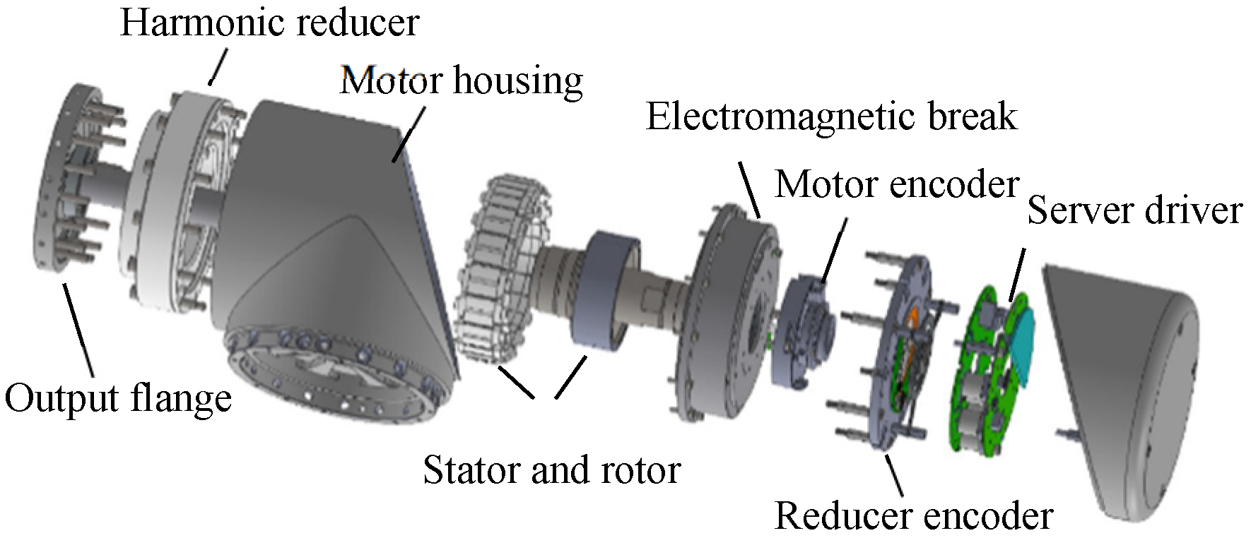
2.1. Structure of Harmonic Reducer

As shown in Figure 2, the harmonic reducer is mainly composed of three components: wave generator, flexible gear, and rigid gear [13].

According to the working principle of harmonic reducers, the meshing effect between the flexible gear and the wave generator can be represented by Fourier series as follows [14,15]:

$$k_{fc}(t)=k_{fc}+{\displaystyle \sum _{i=1}^{\infty }{k}_i}\cos (2\pi i{f}_{c}t+{\psi }_i)$$

(2)

where f_c is the characteristic frequency of the meshing stiffness of the harmonic reducer, i is the order of the Fourier series, k_i is the amplitude corresponding to each Fourier series, ${\psi }_i$ is the phase corresponding to each Fourier series, and k_fc is the meshing stiffness of the harmonic reducer under constant load. In the robot joint module, the wave generator is the input part of the harmonic reducer, driven by a PMSM, with an elliptical shape and a center offset. Therefore, the wave generator generates a periodic fluctuation during rotation. In the OXY coordinate system with the harmonic reducer as the origin, the meshing function between the flexible gear and the wave generator can be expressed as follows:

$$\left\{\begin{array}{l}{k}_{wfx}(t)=k_{x0}+{\displaystyle \sum _{i=2,4,6\dots }^{\infty }{k}_{xi}\cos (2\pi i{f}_n+{\psi }_{xi})}\\ k_{wfy}(t)=k_{y0}+{\displaystyle \sum _{i=2,4,6\dots }^{\infty }{k}_{yi}\cos (2\pi i{f}_n+{\psi }_{yi})}\\ k_{wft}(t)=k_{t0}+{\displaystyle \sum _{i=2,4,6\dots }^{\infty }{k}_{ti}\cos (2\pi i{f}_n+{\psi }_{ti})}\end{array}\right.$$

(3)

where $k_{wfx}(t)$, $k_{wfy}(t)$, $k_{wft}(t)$ are the coupling effect of the x direction, y direction, and rotation direction, $f_n$ is the rotational frequency of the PMSM, ${\psi }_{xi}$, ${\psi }_{yi}$, ${\psi }_{ti}$ are the phases corresponding to Fourier series, $k_{x0}$, $k_{y0}$, $k_{t0}$ are the direct components, and $k_{xi}$, $k_{yi}$, $k_{ti}$ are the amplitudes, respectively. The equation is a periodic function with the rotational frequency of the double-wave generator as the fundamental frequency. The dynamic equation of the wave generator can be described as

$$\left\{\begin{array}{l}{m}_w{\ddot{x}}_w+c_{wx}{\dot{x}}_w+k_{wx}{x}_w=-k_{wfx}(t)(x_w-x_f)-c_{wx}({\dot{x}}_w-{\dot{x}}_f)\\ m_w{\ddot{y}}_w+c_{wy}{\dot{y}}_w+k_{wy}{y}_w=-k_{wfy}(t)(y_w-y_f)-c_{wy}({\dot{y}}_w-{\dot{y}}_f)\\ m_w{\ddot{\theta }}_w+c_{wt}{\dot{\theta }}_w+k_{wt}{\theta }_w=T_{motor}(t)-k_{wft}(t)({\theta }_w-{\theta }_f)-\\ c_{wt}({\dot{\theta }}_w-{\dot{\theta }}_f)\end{array}\right.$$

(4)

where $m_w$ is the quality of the wave generator, $c_{wx}$, $c_{wy}$, $c_{wt}$ are the damping of the wave generator in the x direction, y direction, and rotation direction, respectively, $k_{wx}$, $k_{wy}$, $k_{wt}$ are the stiffness of the wave generator in the x direction, y direction, and rotation direction, respectively, $x_w$, $x_f$ are the vibration displacement of the wave generator in the x and y directions, $y_w$ and $y_f$ are the vibration displacements of the flexible gear in the x and y directions, ${\theta }_w$ and ${\theta }_f$ are the vibration displacements of the rigid gear in the x and y directions, and $T_{motor}(t)$ is the output torque of the PMSM of the joint module. The dynamic equation of the flexible gear can be described as

$$\left\{\begin{array}{c}{m}_f{\ddot{x}}_f+c_{fx}{\dot{x}}_f+k_{fx}{x}_f=k_{wfx}(t)(x_w-x_f)+c_{fx}({\dot{x}}_w-{\dot{x}}_f)\\ +k_{fc}(t)(d_{fc1}-d_{fc2})\cos ({\omega }_{n}t-{\alpha }_{fc})+c_{fc}({\dot{d}}_{fc1}-{\dot{d}}_{fc2})\cos ({\omega }_{n}t-{\alpha }_{fc})\\ m_f{\ddot{y}}_f+c_{fy}{\dot{y}}_f+k_{fy}{y}_f=k_{wfy}(t)(y_w-y_f)+c_{fy}({\dot{y}}_w-{\dot{y}}_f)\\ +k_{fc}(t)(d_{fc1}-d_{fc2})\sin ({\omega }_{n}t-{\alpha }_{fc})+c_{fc}({\dot{d}}_{fc1}-{\dot{d}}_{fc2})\sin ({\omega }_{n}t-{\alpha }_{fc})\\ m_f{\ddot{\theta }}_f+c_{ft}{\dot{\theta }}_f+k_{ft}{\theta }_f=k_{wft}(t)({\theta }_w-{\theta }_f)+c_{ft}({\dot{\theta }}_w-{\dot{\theta }}_f)\\ -k_{fc}(t)(d_{fc1}+d_{fc2})-c_{fc}({\dot{d}}_{fc1}+{\dot{d}}_{fc2})\end{array}\right.$$

(5)

where $m_f$ is the mass of the flexible gear, $c_{fx}$, $c_{fy}$, and $c_{ft}$ are the damping of the flexible gear in the x, y, and rotation directions, $k_{fx}$, $k_{fy}$, and $k_{ft}$ are the stiffness of the flexible gear in the x, y, and rotation directions, ${\alpha }_{fc}$ is the relative displacement angle of the gear mesh, ${\omega }_n$ is the rotational speed of the PMSM, $d_{fc1}$ and $d_{fc2}$ are the displacement values on the equivalent action of the gear, and the expressions are

$$\begin{array}{l}\left\{\begin{array}{l}{d}_{fe1}=-(x_f-x_c)\cos ({\omega }_{n}t-{\alpha }_{fc})-(y_f-y_c)\sin ({\omega }_{n}t-{\alpha }_{fc})\\ +({\theta }_r-{\theta }_c)c_{ft}+e_{fe1}(t)\\ d_{fe2}=(x_f-x_c)\cos ({\omega }_{n}t-{\alpha }_{fc})+(y_f-y_c)\sin ({\omega }_{n}t-{\alpha }_{fc})\\ +({\theta }_r-{\theta }_c)c_{ft}+e_{fe2}(t)\end{array}\right.\end{array}$$

(6)

where $e_{fe1}(t)$ and $e_{fe2}(t)$ are the displacement error forces of gear meshing.

The dynamic equation of a rigid gear can be described as

$$\left\{\begin{array}{c}{m}_c{\ddot{x}}_c+c_{cx}{\dot{x}}_c+k_{cx}{x}_c=-k_{fc}(t)\cos ({\omega }_{n}t-{\alpha }_{fc})(d_{fc1}-d_{fc2})\\ -c_{fc}\cos ({\omega }_{n}t-{\alpha }_{fc})({\dot{d}}_{fc1}-{\dot{d}}_{fc1})\\ m_c{\ddot{y}}_c+c_{cy}{\dot{y}}_c+k_{cy}{y}_c=-k_{fc}(t)\sin ({\omega }_{n}t-{\alpha }_{fc})(d_{fc1}-d_{fc2})\\ -c_{fc}\sin ({\omega }_{n}t-{\alpha }_{fc})({\dot{d}}_{fc1}-{\dot{d}}_{fc1})\\ m_c{\ddot{\theta }}_c+c_{ct}{\dot{\theta }}_c+k_{ct}{\theta }_c=T_{out}(t)+(d_{fc1}+d_{fc2})k_{fc}+({\dot{d}}_{fc1}+{\dot{d}}_{fc2})c_{fc}\end{array}\right.$$

(7)

where $m_c$ is the mass of the rigid gear, $c_{cx}$, $c_{cy}$, and $c_{ct}$ are the damping of the rigid gear in the x, y, and rotation directions, respectively, and $k_{cx}$, $k_{cy}$, and $k_{ct}$ are the stiffness of the rigid gear in the x, y, and rotation directions, respectively.

2.2. Dynamic Response Analysis of Robot Joint Module

In the structure of the robot joint module, vibration mainly comes from the unstable contact between the flexible gear and the wave generator, the periodic variation in the tooth contact force between the flexible gear and the rigid gear, and the elastic deformation of the flexible gear [5]. As described in (4), the vibration of the flexible gear is mainly in the x direction, y direction, and rotational direction. This is mainly caused by factors such as the fluctuation of the tooth contact force between the flexible gear and the rigid gear, and the fluctuation of the driving torque.

The vibrations in these three directions may interact with each other, forming complex vibration patterns. In the study of robot vibration, y direction vibration is easy to measure, so further analysis is needed for the y direction vibration in (4).

According to (4), the dynamic equation of the flexible gear in the y direction is

$$\begin{array}{c}{m}_f{\ddot{y}}_f+c_{fy}{\dot{y}}_f+k_{fy}{y}_f=k_{wfy}(t)(y_w-y_f)+c_{fy}({\dot{y}}_w-{\dot{y}}_f)\\ +k_{fc}(t)(d_{fc1}-d_{fc2})\sin ({\omega }_{n}t-{\alpha }_{fc})+c_{fc}({\dot{d}}_{fc1}-{\dot{d}}_{fc2})\sin ({\omega }_{n}t-{\alpha }_{fc})\end{array}$$

(8)

Substituting (6) into (7) and classifying the nonlinear damping change as an unknown perturbation quantity for processing, one can have

$$m_f{\ddot{y}}_f+c_{fy}{\dot{y}}_f+k_{fy}{y}_f=(e_{fc1}(t)-e_{fc2}(t))k_{fc}(t)\sin ({\omega }_{n}t-{\alpha }_{fc})$$

(9)

$$m_f{\ddot{y}}_f+c_{fy}{\dot{y}}_f+k_{fy}{y}_f=(y_f-y_c)k_{fc}(t)[\cos 2({\omega }_{n}t-{\alpha }_{fc})-1]$$

(10)

$$m_f{\ddot{y}}_f+c_{fy}{\dot{y}}_f+k_{fy}{y}_f=(y_w-y_f)k_{wfy}(t)$$

(11)

The right-hand term $(y_w-y_f)k_{wfy}(t)$ in (10) reflects the magnitude of the excitation force on the flexible gear and is a nonlinear equation. As described in (3) and (4), variables $y_w$ and $y_f$ describe the vibration displacement of the flexible gear in different directions, and $k_{wfy}(t)$ is the meshing function of the flexible gear in the y direction. In fact, it is impossible to accurately obtain the actual data of y_w and y_f in (11), nor can it obtain the accurate data of the nonlinear equation $k_{wfy}(t)$. From the analysis of the force on the flexible gear, the force $(y_w-y_f)k_{wfy}(t)$ includes the synthesis of the load disturbance force on the flexible gear and various vibration disturbance forces.

Let $f_t(t)+T(t)=(y_w-y_f)k_{wfy}(t)$, where $f_t(t)$ is the vibration impact force of the flexible gear itself, and $T(t)$ is the load disturbance force acting on the flexible gear. It is approximately equivalent to the combined force of the load disturbance force and various vibrations. The reason that this combined force is used will be further explained in the ${\theta }_{e1}(t)$ experimental waveform in Section 3. Therefore, one can have

$$m_f{\ddot{y}}_f+c_{fy}{\dot{y}}_f+k_{fy}{y}_f=f_t(t)+T(t)$$

(12)

where $f_t(t)+T(t)$ is the total excitation force of the flexible gear, which is related to the load, mass, damping, stiffness, vibration displacement of the flexible gear, including the load disturbance force and vibration impact force of the flexible gear, and is a nonlinear function.

In vibration analysis, the robot joint module can be considered as a whole. By extending (11), the general form of the vibration equation can be written as

$$m\ddot{y}(t)+c\dot{y}(t)+ky(t)=f(t)+T_{load}(t)$$

(13)

where m is the mass of the joint module, c is the damping of the joint module, k is the stiffness of the joint module, and y(t) is the displacement. $\ddot{y}(t)$ is the vibration velocity. $T_{load}(t)$ is the vibration acceleration. $T_{load}(t)$ is the load disturbance force of the joint module, and $f(t)$ represents the vibration impact force of the joint module, which can be measured by installing vibration sensors on the robot joint module. However, this method has some inconveniences [10].

3. ADRC Control of Robot Joint Module

In order to reduce the vibration of robot joint modules, the following methods can be considered [16]: (1) adjust the frequency of the external force, (2) increase the damping of the robot system, (3) adjust the stiffness of the system, and (4) optimize the control algorithm, such as the adaptive control, fuzzy control, or predictive control, to reduce vibration. This article uses the ADRC algorithm for vibration suppression, and the control structure is shown in Figure 3 [17], including the tracking differentiator (TD), linear state error feedback (LSEF), and extended state observer (ESO).

3.1. Vibration Disturbance Model of Joint Module

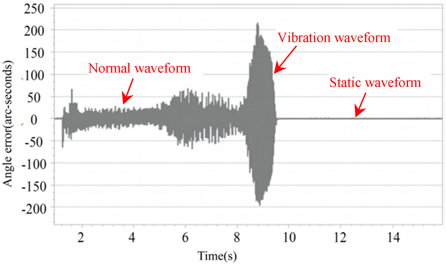
3.1.1. Extraction of Vibration Signals

As shown in Figure 1, two encoders are installed on the robot joint module. The reduction ratio is N.

For the convenience of vibration analysis, a simplified model is adopted for the mechanical part of the joint module, as shown in Figure 4, whose forces are manifested as the meshing vibration and elastic deformation between gears. Then, the following equation is introduced.

$$\left\{\begin{array}{l}{\theta }_{e1}(t)={\theta }_0(t)-N{\theta }_r(t)\\ {\omega }_{e1}(t)={\omega }_0(t)-N{\omega }_r(t)\\ a_{e1}(t)=a_0(t)-N{a}_r(t)\end{array}\right.$$

(14)

where ${\theta }_0(t)$ is the motor angle, ${\omega }_0(t)$ is the motor speed, $a_0(t)$ is the motor angular acceleration, ${\theta }_r(t)$ is the harmonic reducer angle, ${\omega }_r(t)$ is the harmonic reducer speed, $a_r(t)$ is the harmonic reducer angular acceleration, and ${\theta }_{e1}(t)$ is the difference between the theoretical and actual positions of the robot joint module.

Then, one can have

$$\left\{\begin{array}{l}{\omega }_0(t)={\dot{\theta }}_0(t)\\ a_0(t)={\ddot{\theta }}_0(t)\end{array}\right.$$

(15)

$$\left\{\begin{array}{l}{\omega }_r(t)={\dot{\theta }}_r(t)\\ a_r(t)={\ddot{\theta }}_r(t)\end{array}\right.$$

(16)

From (14)–(16), it can be concluded that

$$\left\{\begin{array}{l}{\omega }_{e1}(t)={\dot{\theta }}_{e1}(t)\\ a_{e1}(t)={\ddot{\theta }}_{e1}(t)\end{array}\right.$$

(17)

When the rigidity of the robot joint module is sufficiently high and there is no vibration disturbance, ${\theta }_0(t)-N{\theta }_r(t)=0$, ${\theta }_{e1}(t)=0$. The angle output of the PMSM is completely synchronized with the angle output of the harmonic reducer. When considering the existence of gear deformation and load vibration, the joint module exhibits a nonlinear output of ${\theta }_{e1}(t)$ during rotation. A sampling interval of 1 millisecond and collected data from the two encoders of the joint module are selected to generate ${\theta }_{e1}(t)$ data, as shown in Figure 5. The horizontal axis represents time, and the vertical axis represents ${\theta }_{e1}(t)$, which is the angle error value, in arcseconds.

Figure 5 shows the waveforms of the joint module during the normal operation, vibration, and static state, which approximate the synthesis of the load deformation displacement data and vibration displacement data. By combining (13), (14) and (17), one can have

$$m\alpha {\ddot{\theta }}_{e1}(t)+c\alpha {\dot{\theta }}_{e1}(t)+k\alpha {\theta }_{e1}(t)=f(t)+T_{load}(t)$$

(18)

where $T_{load}(t)$ represents the load disturbance force of the joint module, $f(t)$ represents the vibration impact force of the joint module, and $\alpha$ is an undetermined coefficient that needs to be adjusted through an ADRC controller.

The latter half of Figure 5 shows that in a static and vibration-free state, ${\ddot{\theta }}_{e1}(t)=0$ and ${\dot{\theta }}_{e1}(t)=0$ in (18) describe the vibration acceleration and velocity. Therefore, (18) is further decomposed into

$$\left\{\begin{array}{l}{T}_{load}(t)=k\alpha {\theta }_{e1}(t)\\ f(t)=m\alpha {\ddot{\theta }}_{e1}(t)+c\alpha {\dot{\theta }}_{e1}(t)\end{array}\right.$$

(19)

It should be noted that (19) simplifies the force situation of the joint module, such as linear and time invariance, and ignores some possible nonlinear and time-varying effects, such as the nonlinearity of tooth contact and the time variation in the stiffness and damping.

3.1.2. Vibration Model Analysis of Robot Joint Module

In (19), it is necessary to determine the parameters of the damping ratio and stiffness. The derivation of these two parameters is based on second-order linear differential equations and used to describe the dynamic response of joint module vibration [18].

According to (13), the robot joint module model can be described using a simplified second-order differential equation

$$m\ddot{y}(t)+c\dot{y}(t)+ky(t)=u(t)$$

(20)

where m is the mass, c is the damping coefficient, k is the stiffness coefficient, and y(t) is the displacement response of the system. By conducting static loading experiments and dynamic response experiments on harmonic reducers, data for k and c can be obtained separately [19,20].

The above differential equation can be converted into a standard second-order differential equation form

$$\ddot{y}(t)+{\displaystyle \frac{c}{m}}\dot{y}(t)+{\displaystyle \frac{k}{m}}y(t)={\displaystyle \frac{1}{m}}u(t)$$

(21)

3.2. ESO Design

The ESO is a key component of the ADRC algorithm. The main function of the ESO is to estimate the internal state and total disturbances of the system in real time, including model uncertainty and external disturbances.

3.2.1. Mathematical Model of PMSM

When factors such as magnetic saturation, hysteresis damage, and eddy current losses are ignored, the stator voltage equation of the PMSM in a dq coordinate system can be described as [21]

$$\left\{\begin{array}{l}{u}_d=R_s{i}_d-{\omega }_e{L}_q{i}_q+L_d{\displaystyle \frac{\mathrm{d}{i}_d}{\mathrm{d}t}}\\ u_q=R_s{i}_q+{\omega }_e{L}_d{i}_d+{\omega }_e{\psi }_f+L_q{\displaystyle \frac{\mathrm{d}{i}_q}{\mathrm{d}t}}\end{array}\right.$$

(22)

The electromagnetic torque equation is

$$T_e^{\ast }={\displaystyle \frac{3}{2}}{n}_p{\psi }_f{i}_q$$

(23)

The equation of motion is

$$J{\displaystyle \frac{\mathrm{d}{\omega }_0}{\mathrm{d}t}}=T_e^{\ast }-T_{load}$$

(24)

where $u_d$ and $u_q$ are the d axis and q axis components of the stator voltage, i_d and i_q are the d axis and q axis components of the stator current, $n_p$ is the number of pole pairs, ${\phi }_f$ is the rotor magnetic flux, ${\omega }_e$ is the rotor electrical angular velocity, and ${\omega }_e=n_p{\omega }_0$. ${\omega }_0$ are the motor angular velocity, J is the moment of inertia, $T_e^{\ast }$ is the electromagnetic torque, and $T_{load}$ is the load torque [22,23].

When considering the disturbance term and damping term, (24) can be rewritten as

$$J{\displaystyle \frac{\mathrm{d}{\omega }_0}{\mathrm{d}t}}=T_e^{\ast }-T_{load}-\stackrel{⌢}{d}(t)$$

(25)

where $\stackrel{⌢}{d}(t)$ is the estimated disturbances that include the damping disturbances, vibrational impact disturbances, and sudden load variations, among others.

These disturbances encompass nonlinear factors and exhibit time-varying characteristics, making precise modeling challenging. Consequently, the ADRC theory treats both internal and external nonlinearities and all kinds of disturbances including the frictional forces and other force disturbances you mentioned as a unified “total disturbance,” which is estimated and compensated in real time, thereby reducing reliance on model accuracy.

The core procedure primarily involves the design of an ESO: it treats unmodeled dynamics, nonlinear friction, external disturbances, etc., as total disturbance and provides real-time estimation of the total disturbance through the state observer.

3.2.2. Speed Loop ESO Design

According to the motor motion equation, with ${\omega }_0$, ${\theta }_0$, and ${\theta }_{e1}$ as state variables, the state equation of the robot integrated joint module is written as

$$\left\{\begin{array}{l}{\dot{\theta }}_0={\omega }_0\\ {\dot{\omega }}_0=f(t)+f_n(t)+b_0{T}_e^{\ast }\\ f(t)=m\alpha {\ddot{\theta }}_{e1}(t)+c\alpha {\dot{\theta }}_{e1}(t)\\ f_n(t)=-b_0{T}_{load}(t)-b_{0}B({\omega }_0-{\widehat{\omega }}_0)+n_n(t)\end{array}\right.$$

(26)

where ${\theta }_0$ is the motor angle, ${\omega }_0$ is the motor speed, B is the motor damping, $\alpha$ and $b_0$ are the ESO parameters, ${\theta }_{e1}(t)$ is the difference between the theoretical and actual positions of the robot joint module, m is the mass of the joint module, c is the damping of the joint module, ${\widehat{\omega }}_0$ is the estimated speed, $n_n(t)$ is other unmodeled dynamic terms, $f(t)$ is the vibration disturbance, and $f_n(t)$ represents other unknown disturbances [24].

The unknown disturbance $f_n(t)$ includes the torque disturbance term of the load, other unmodeled dynamic terms $n_n(t)$, and the mismatch between the estimated speed value ${\widehat{\omega }}_0$ and the actual motor speed value. This mismatch is related to the assembly accuracy of the encoder and the delay in data communication transmission. This article used a Nikon photoelectric encoder, which uses the 485 communication protocol and a communication transmission delay time of 40 μs. The higher the motor speed, the greater the disturbance of the communication transmission delay on speed calculation.

The ESO is used to observe the velocity signal in (26), the unknown disturbance term $f_n(t)$ of the robot joint module is expanded to a new state variable as follows.

$$\left\{\begin{array}{l}{\dot{\theta }}_0={\omega }_0\\ {\dot{\omega }}_0=f(t)+f_n(t)+b_0{T}_e^{\ast }\\ f(t)=m\alpha {\ddot{\theta }}_{e1}(t)+c\alpha {\dot{\theta }}_{e1}(t)\\ {\dot{f}}_n(t)=h_n(t)\end{array}\right.$$

(27)

where $h_n(t)$ is the derivative of an unknown perturbation term.

The standard form of the third-order ESO based on (26) and (27) is written as

$$\left\{\begin{array}{l}{e}_{1n}=z_{1n}-{\theta }_0\\ {\dot{z}}_{1n}=z_{2n}-{\beta }_{1n}{e}_{1n}\\ {\dot{z}}_{2n}=z_{3n}+f_n+b_0{T}_e^{\ast }-{\beta }_{2n}{e}_{1n}\\ {\dot{z}}_{3n}=-{\beta }_{3n}{e}_{1n}\end{array}\right.$$

(28)

where $e_{1n}$ is the angle error value, $z_{1n}$ is the estimated value of ${\theta }_0$, $z_{2n}$ is the estimated value of ${\omega }_0$, $z_{3n}$ is the estimated value of the unknown disturbance term $f_n$, and $b_0$, ${\beta }_{1n}$, ${\beta }_{2n}$, and ${\beta }_{3n}$ are the parameters of the ESO [25].

3.2.3. Mathematical Stability Analysis of ADRC

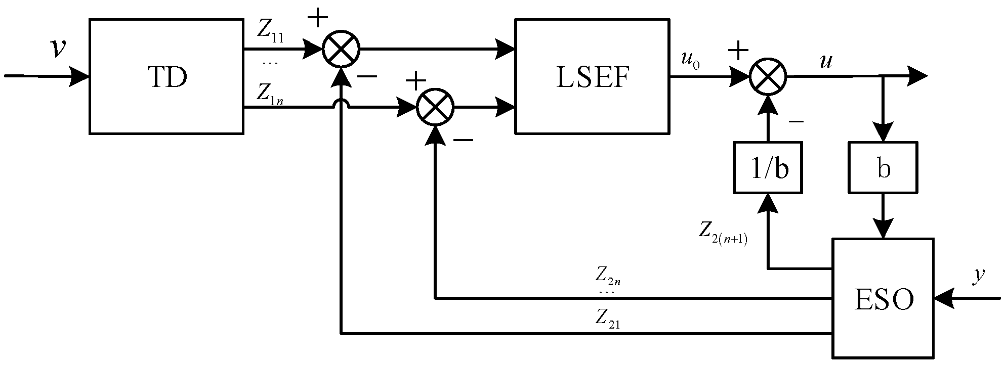
The theoretical basis of ADRC mainly comes from the work of Professor Han, who first proposed the core concept of an ESO but did not provide strict mathematical proof. In the subsequent studies of scholars, the convergence of an ESO has been further proved. For instance, Zhao et al. studied the relationship between the stability of the ESO bandwidth and the system cut-off frequency, and for the first time established the convergence theory of an ESO based on frequency-domain analysis and the Lyapunov method [26,27].

The design of an ESO can usually be expressed as

$$\left\{\begin{array}{l}{e}_1=z_1-x_1\\ {\dot{z}}_1=z_2-{\beta }_1{e}_1\\ {\dot{z}}_2=z_3-{\beta }_2{e}_{1n}+b_{0}u\\ {\dot{z}}_{3n}=-{\beta }_{3n}{e}_{1n}\end{array}\right.$$

(29)

When the bandwidths of an ESO satisfy ${\omega }_0>3{\omega }_c$, ${\omega }_c$ is the cut-off frequency, the estimation error satisfies

$$\underset{t\to \infty }{\lim }|z_i(t)-x_i(t)|<=O({\displaystyle \frac{1}{{\omega }_0^i}})$$

(30)

where $z_i$ is the estimation of the system state and disturbance, $x_i$ is the input signal, $e_i$ is the estimation error, and $O(x)$ is the upper bound of the estimation error proportional to the negative power of ${\omega }_0$. The disturbance suppression conditions in the stability analysis are

$$|\tilde{d}(t)|=|z_3-d(t)|<=\epsilon$$

(31)

where $\tilde{d}(t)$ is the total perturbation estimation residual, $d(t)$ is the perturbation value, $\epsilon$ is the perturbation suppression accuracy threshold, and ${\omega }_0$ is positively correlated with the ESO bandwidth.

3.2.4. LSEF Design

The design requirement of LSEF is that the expected $e_{1n}$ should be as close to zero as possible in both steady-state and dynamic processes. The forward channel error of LSEF is defined as $e_{LSEF}$, which is the error between the given speed value and the estimated speed value

$$e_{LSEF}={\omega }_0^{\ast }-z_{2n}$$

(32)

where ${\omega }_0^{\ast }$ is the given command value for the rotational speed.

The equation of state is

$${\dot{e}}_{LSEF}={\dot{\omega }}_0^{\ast }-{\dot{z}}_{2n}={\dot{\omega }}_0^{\ast }-(z_{3n}+f_n+b_0{T}_e^{\ast }-{\beta }_{2n}{e}_{1n})$$

(33)

where $a_0^{\ast }$ is defined as the command value for the given angular acceleration of the motor, which is obtained through TD based on the given speed command ${\omega }_0^{\ast }$. The difference between the speed acceleration command and the disturbance command is used for feedforward control, to suppress vibration disturbances during the dynamic process of the speed loop, thereby improving system performance.

That is

$$a_0^{\ast }={\dot{\omega }}_0^{\ast }$$

(34)

Combining (35) and (36), LSEF is designed as

$$T_e^{\ast }={\displaystyle \frac{k_{ps}({\omega }_0^{\ast }-z_{2n})+k_{is}\int ({\omega }_0^{\ast }-z_{2n})dt-(a_0^{\ast }-(f_n+f))}{b_0}}$$

(35)

where $k_{ps}$ and $k_{is}$ are the proportion and integration coefficient of the LSEF controller, respectively [28,29].

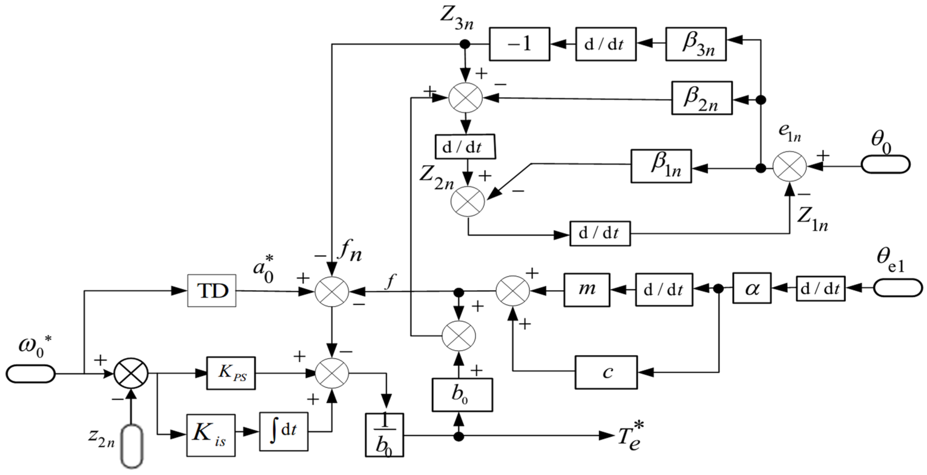
3.3. ADRC Control Strategy

According to (27), (29) and (31), the ADRC block diagram is designed as shown in Figure 6.

Figure 7, Figure 8 and Figure 9 show the simulation experiments, where the red and blue lines represent the joint speed fluctuation and current fluctuation values of the FOC algorithm and ADRC algorithm, respectively. The simulation results show that after adding the ADRC algorithm, the speed fluctuation at 100 rpm of the joint is reduced by 60%, the speed fluctuation at 1000 rpm is reduced by 40%, and the torque current fluctuation is reduced by 50%.

4. Comparison and Analysis of Experimental Results

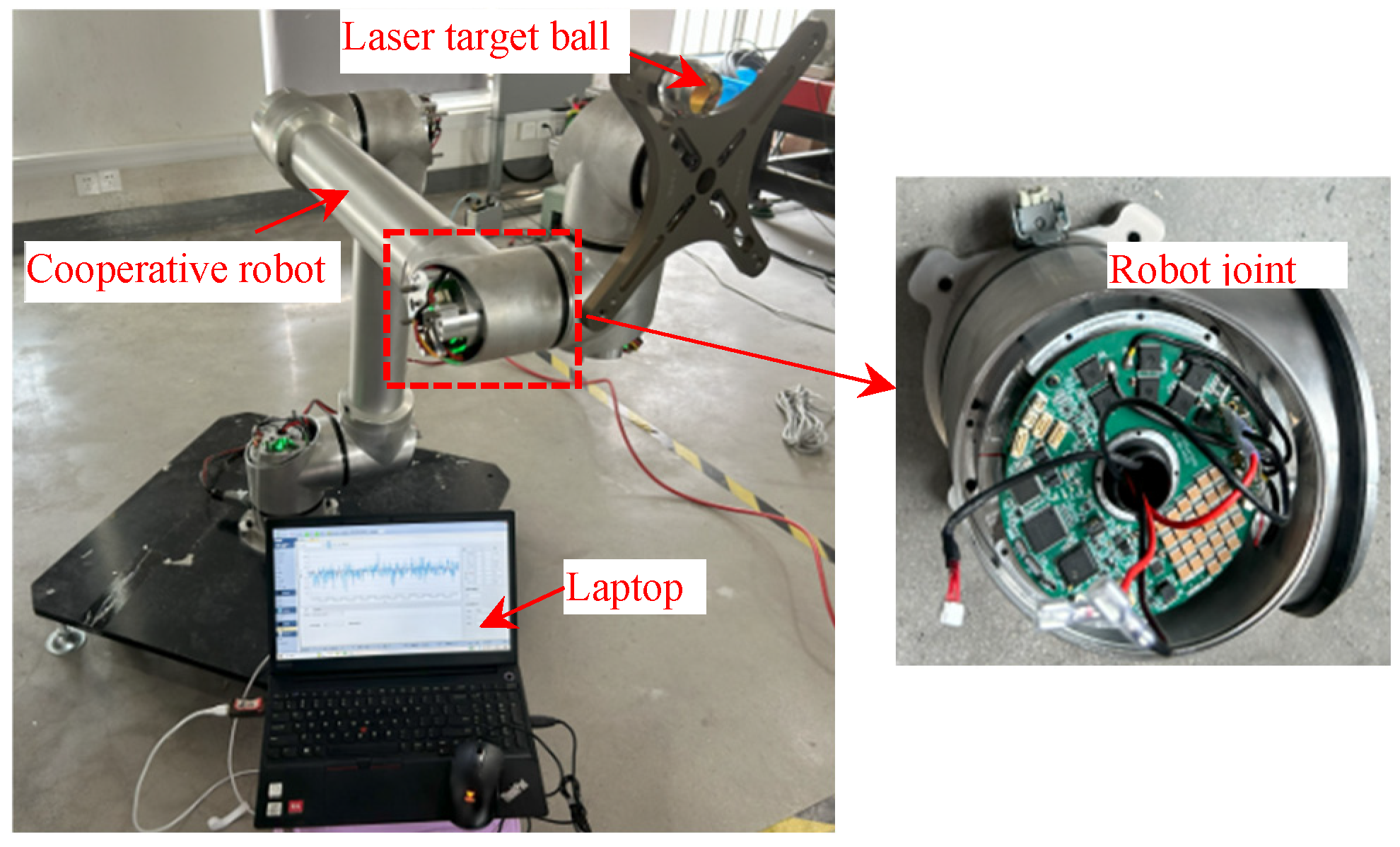
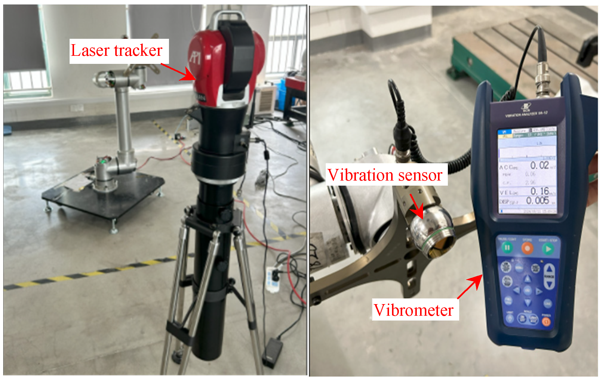
4.1. Experimental Setup and Methods

4.1.1. Robot Integrated Joint Module and Collaborative Robot

In order to verify the correctness of the proposed algorithm, a platform was built as follows. Figure 10 shows the collaborative robot used in the experiment. The electrical parameters are listed in

Table 1. Joint parameter.

Item	Parameters	Unit
Rated speed	1500	rpm
Rated current	19.4	A
Rated torque	3.32	N∙m
Phase resistance	0.25	ohms
Phase inductance	4.9	mH
Back electromotive force	13.6	Vrms/krpm
Encoder resolution	20	bit
Harmonic reducer transmission ratio	1:81
Rated torque of harmonic reducer	107	N∙m
Peak torque of harmonic reducer	169	N∙m
Positioning accuracy	25	arcseconds

.

Figure 11 shows the installation of a laser target ball on the end of the machine, and the use of a laser tracker to collect trajectory velocity fluctuations. At the same time, a vibrometer was installed at the end of the robot to record vibration data.

4.1.2. Experimental Results and Analysis

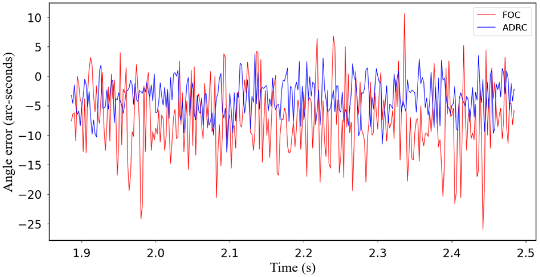
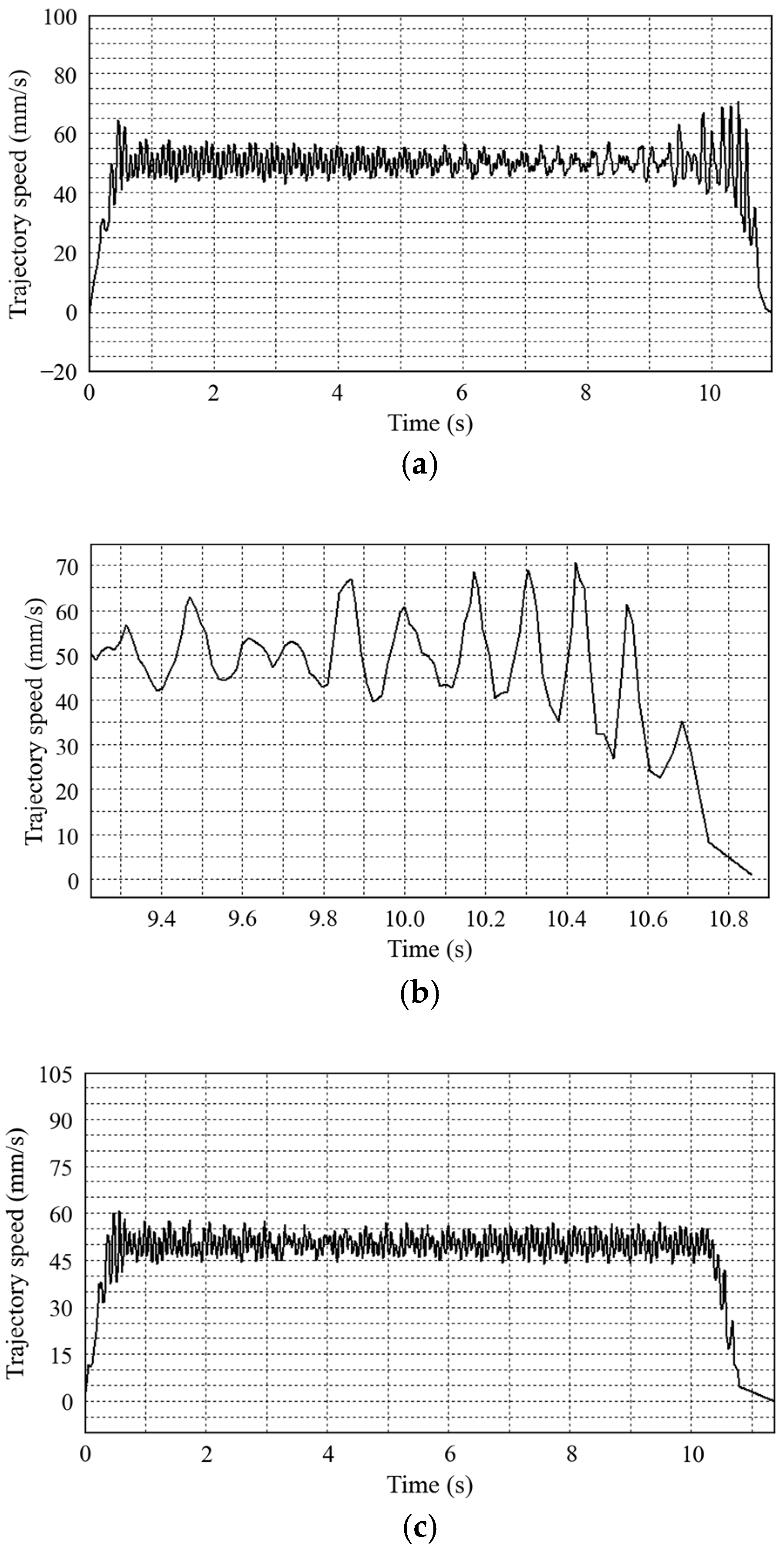
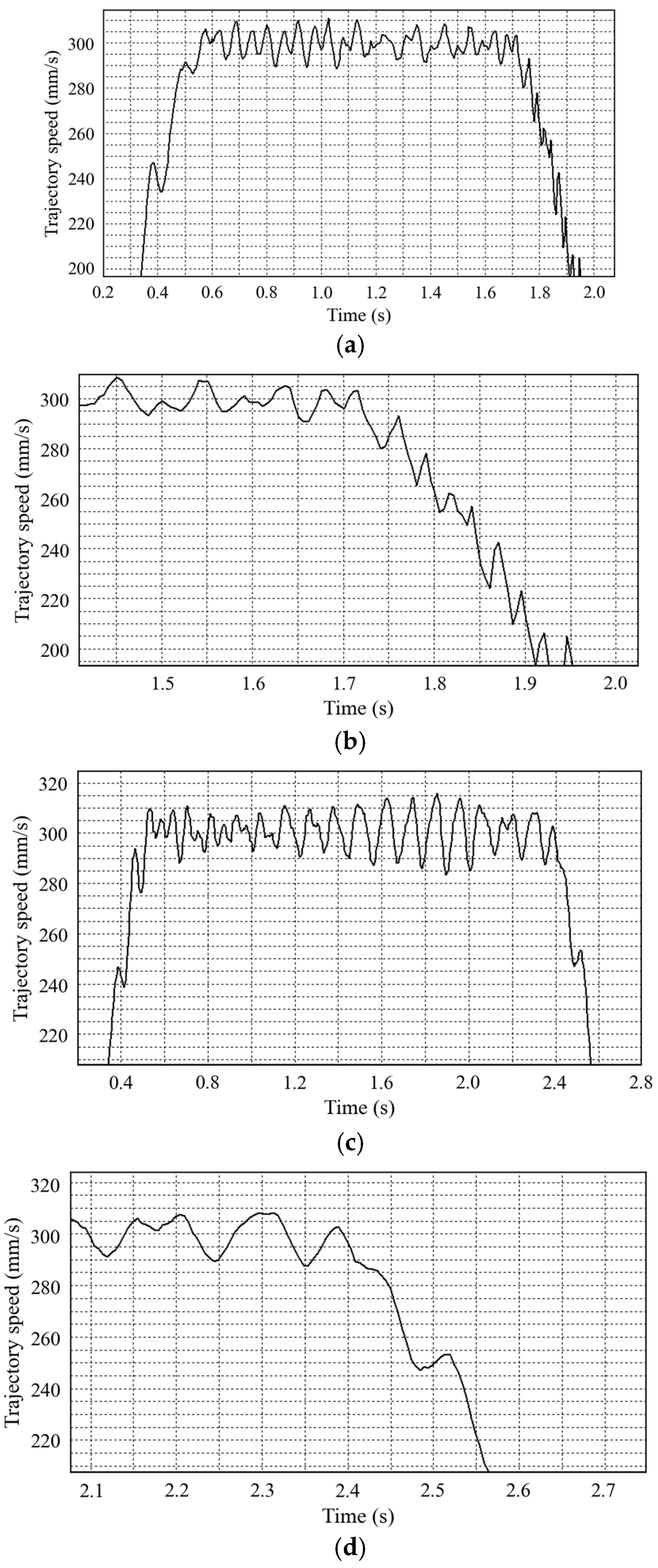
The vibration of robot motion trajectory is usually caused by the velocity fluctuation of one of the joints. During the experiment, six joints of the robot were made to work together to move along a straight path, and the following data were recorded for comparison and reference:

(1)

Robot trajectory jitter waveform.

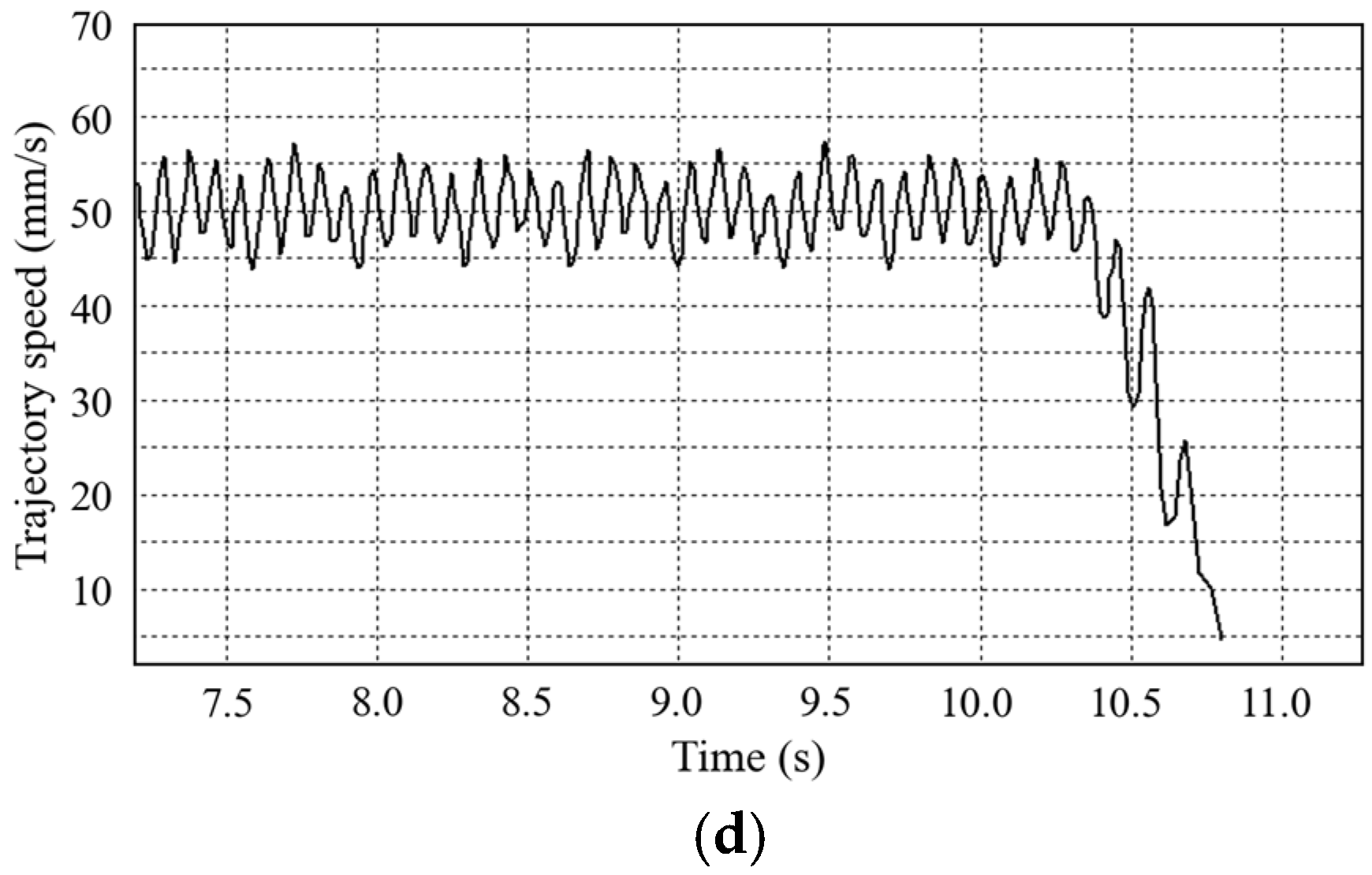
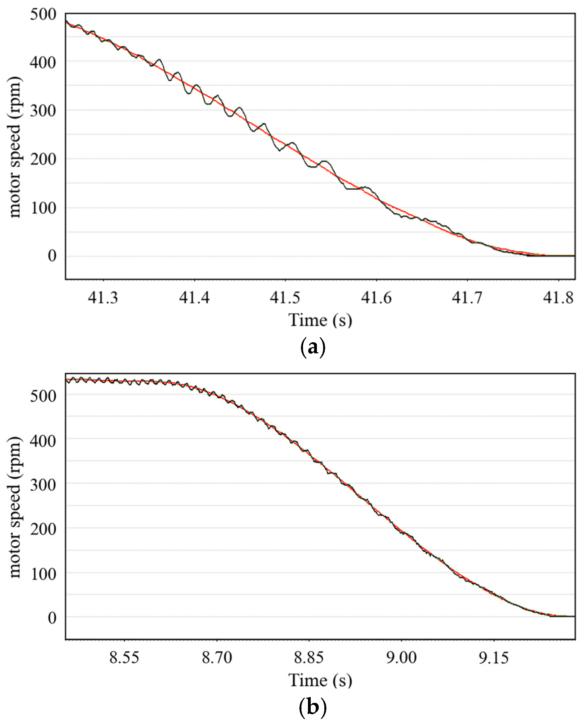
(2)

Velocity waveform of robot joint module PMSM.

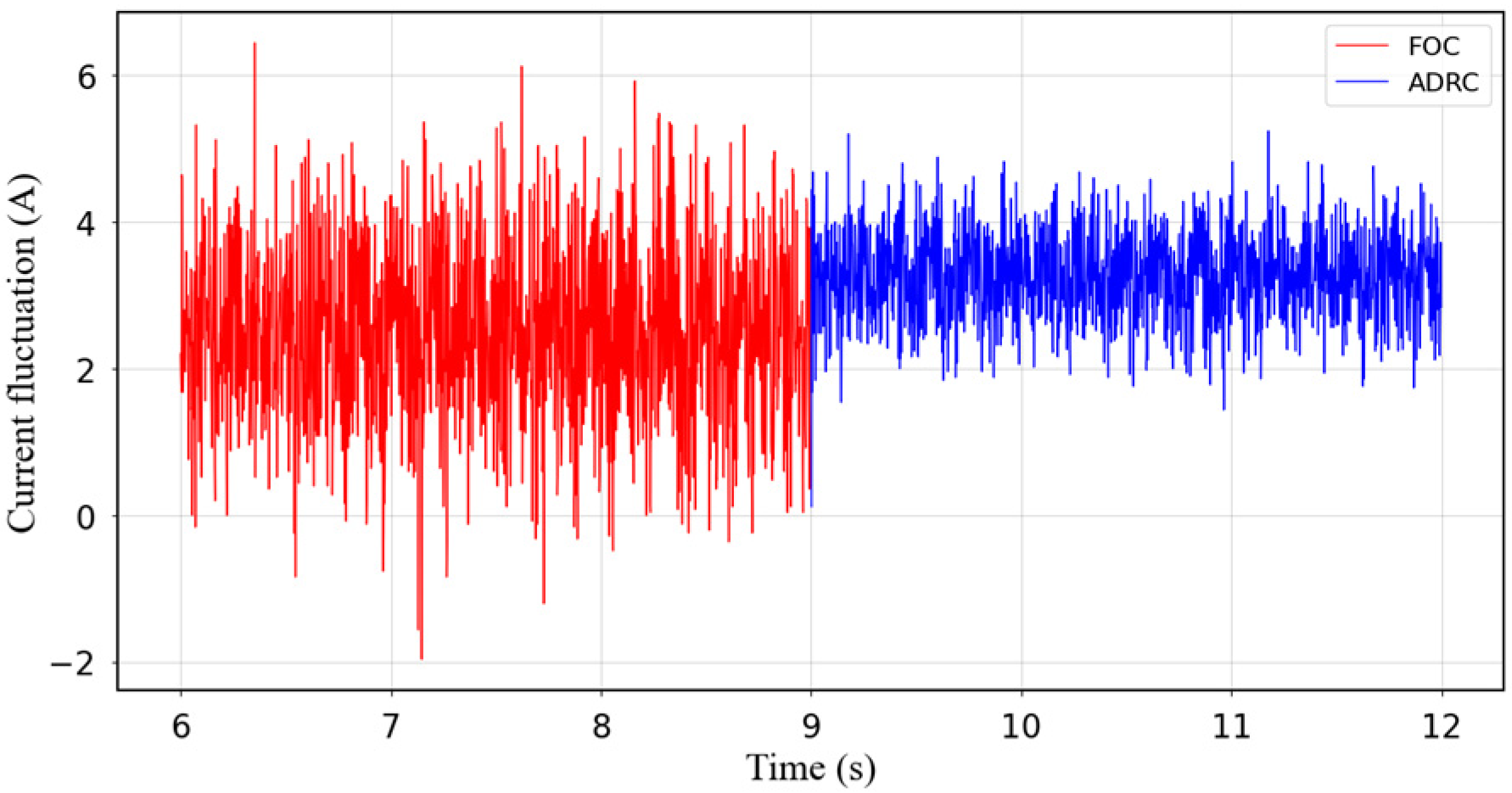
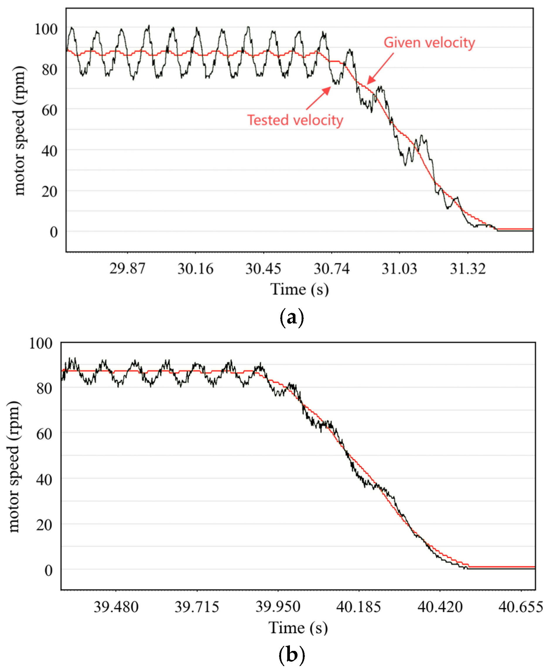
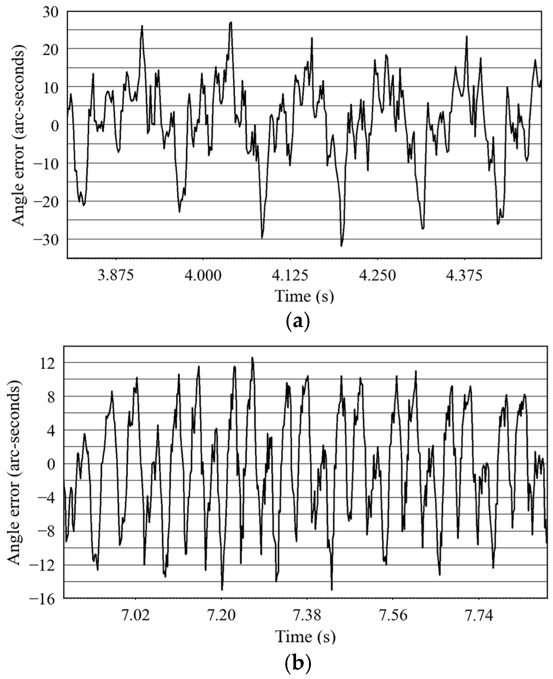
(3)

${\theta }_{e1}(t)$ data waveform.

(4)

The vibration peak data read by the vibrometer.

The rationality of vibration suppression is verified by controlling the fluctuation value of ${\theta }_{e1}(t)$ through these four related data. It was found that the velocity fluctuation of the second joint was significantly higher than that of the other five joints. Therefore, this experiment will focus on comparing and analyzing the vibration data of the second joint.

In order to investigate the influence of different trajectory velocities on vibration, two trajectory velocities were selected to compare the effects of adding the ADRC algorithm, namely 50 mm/s and 300 mm/s.

A.

Experimental results of 50 mm/s

Figure 12 shows the speed fluctuation of the robot trajectory running at a speed of 50 mm/s. The horizontal axis in the figure represents the time coordinate in seconds, and the vertical axis represents the velocity value of the trajectory captured by the laser tracker in millimeters per second.

As shown in Figure 12a,b, when using the vector control algorithm, the maximum trajectory velocity fluctuation occurs during the transition of the robot from uniform speed to deceleration, with a trajectory fluctuation value of plus or minus 20 mm/s. Figure 12c,d show the significant improvement in trajectory fluctuations of the robot joint module after applying the ADRC algorithm, with the fluctuation amplitude successfully reduced to plus or minus 5 mm/s. These data clearly reflect the effectiveness of the ADRC algorithm in improving robot motion stability.

Figure 13 shows the PMSM velocity waveform of the second joint when the robot trajectory speed is set to 50 mm/s. The red line in the waveform corresponds to the speed setting value of the PMSM, while the green line reflects the actual speed value of the PMSM. When the robot performs linear motion at a speed of 50 mm/s, if the vector control algorithm is used, the speed fluctuation range of the PMSM is plus or minus 11 revolutions per minute, as shown in Figure 13a. After applying the ADRC algorithm, the speed fluctuation significantly decreased to plus or minus 5 revolutions per minute, as shown in Figure 13b.

Figure 14 shows the angle error ${\theta }_{e1}(t)$ waveform exhibited by the second joint of the robot under the condition that the robot trajectory running speed is set to 50 mm/s. Specifically, when using the vector control algorithm, the fluctuation range of ${\theta }_{e1}(t)$ is plus or minus 25 arcseconds, as shown in Figure 14a. After applying the ADRC algorithm, the fluctuation range of ${\theta }_{e1}(t)$ was significantly reduced to plus or minus 9 arcseconds, as shown in Figure 14b. This comparison result demonstrates the superiority of the ADRC algorithm in reducing angle error fluctuations.

The vibration data are listed in

Table 2. Comparison of control results for robots running at 50 mm/s speed.

Algorithm	Vector Control	ADRC
Robot trajectory speed	50 mm/s	50 mm/s
Trajectory speed fluctuation	±20 mm/s	±5 mm/s
Joint PMSM speed fluctuation	±11 rpm	±5 rpm
Joint angle error ${\theta }_{e1}(t)$	±25 arcseconds	±9 arcseconds
Amplitude	0.599 mm	0.231 mm
Vibration velocity	9.65 mm/s	4.77 mm/s
Vibration acceleration	0.47 m/s2	0.33 m/s2

for further analysis and research.

B.

Experimental results of 300 mm/s

Figure 15 shows the trajectory fluctuation of the robot when running at a speed of 300 mm/s. Figure 16 shows the speed fluctuation of the PMSM when the robot trajectory begins to decelerate at a speed of 300 mm/s.

Figure 17 shows the angle error ${\theta }_{e1}(t)$ waveform exhibited by the robot joints under the condition that the robot trajectory running speed is set to 300 mm/s. The data are summarized in

Table 3. Comparison of control results for robots running at 300 mm/s speed.

Algorithm	Vector Control	ADRC
Robot trajectory speed	300 mm/s	400 mm/s
Fluctuations during trajectory deceleration	±11 mm/s	±4 mm/s
Joint PMSM speed fluctuation	±12 rpm	±5 rpm
Joint angle error ${\theta }_{e1}(t)$	±28 arcseconds	±13 arcseconds
Amplitude	0.322 mm	0.311 mm
Vibration velocity	8.32 mm/s	6.86 mm/s
Vibration acceleration	1.19 m/s2	0.52 m/s2

.

Through the optimization of the ADRC algorithm and the summarization of the experimental data, the following results can be obtained: The fluctuation values of the robot trajectory speed, joint speed, and joint angle error can be reduced to a maximum of 20.0%, 53.3%, and 35.3% of their original values, respectively. The vibration indicators of robot joints, such as the amplitude, vibration velocity, and vibration acceleration, can be reduced to a maximum of 30.9%, 23.4%, and 24.6% of their original values, respectively. Compared with the traditional FOC algorithm, ADRC exhibits significant advantages.

In the field of robot vibration suppression, traditional control methods and emerging algorithms each have their own characteristics. Theories such as input shaping algorithms, model predictive control, modeling based on the finite element method, and online gravity compensation all require the establishment of precise mathematical models. However, in robot control, the presence of nonlinear factors and time-varying disturbances within the system suppresses the effectiveness of precise model-based control. The ADRC vibration suppression method, by employing the ESO to regard internal nonlinear variations and external disturbances as a “total disturbance” and compensate for it in real time, does not rely on high-precision models. Nevertheless, adjusting the parameters of ADRC is relatively challenging and depends on experience or trial-and-error methods. When the application scenarios of robots vary, parameters need to be adjusted online, and currently, there is a lack of a systematic adaptive mechanism. This is also a difficulty in promoting ADRC theory. The next step of this research will be dedicated to the integration of artificial intelligence with ADRC, adopting machine learning algorithms to enable robot joints to automatically search for the optimal parameters of ADRC.

5. Conclusions

This article proposes a novel vibration suppression strategy, which successfully extracts vibration disturbance signals by accurately measuring the angle error values of robot joints, conducting in-depth analysis of the reducer model, and redesigning the ESO. These disturbance signals are then introduced into the speed loop controller of the PMSM, effectively reducing the fluctuation of the robot joint angle error values. The experimental results have verified the feasibility and effectiveness of this method, significantly reducing the vibration level of the robot and providing a new type of technical support for precise control of the robot.

As an advanced control method that does not rely on an accurate system model and can actively estimate and compensate for disturbances, ADRC demonstrates unique theoretical value and application potential in the field of robot vibration suppression. In response to the challenge of precisely modeling the complex disturbances in robot systems, such as nonlinearity, flexibility deformation, and external interferences, this article employs a unified framework of “total disturbance”. Through the ESO, the unmodeled dynamics, nonlinear coupling effects, and external disturbances are regarded as external state variables of the system and are estimated and dynamically compensated for in real time. The core advantage of this approach is breaking through the dependence of traditional control methods on high-precision dynamic models. Even in the presence of parametric uncertainties and time-varying characteristics in the system, the ESO can still effectively track the changes in disturbances, thereby significantly enhancing the robustness of vibration suppression. Experimental and theoretical studies have shown that ADRC is widely applicable to nonlinear and time-varying robot systems and provides an effective solution for vibration suppression across different speed scenarios.

The adjustment of the ADRC parameters used in this study is rather difficult. A great deal of effort was spent on the experiment to adjust the ADRC parameters. Currently, these parameters are attempted to be adjusted based on the author’s personal practical experience, which is also the difficulty in the promotion of ADRC theory.

The next research work of this paper will focus on the combination of artificial intelligence and ADRC, adopting a machine learning algorithm to enable the robot joint to automatically find the optimal parameters of ADRC.

References

1. Javaid, M.; Haleem, A.; Singh, R.P.; Suman, R. Substantial capabilities of robotics in enhancing industry 4.0 implementation. Cogn. Robot. 2021, 1, 58–75. [Google Scholar] [CrossRef]
2. Islam, R.U.; Iqbal, J.; Manzoor, S.; Khalid, A.; Khan, S. An autonomous image-guided robotic system simulating industrial applications. In Proceedings of the 2012 7th International Conference on System of Systems Engineering (SoSE), Genova, Italy, 16–19 July 2012; pp. 344–349. [Google Scholar] [CrossRef]
3. Erden, M.S.; Billard, A. Hand impedance measurements during interactive manual welding with a robot. IEEE Trans. Robot. 2015, 31, 168–179. [Google Scholar] [CrossRef]
4. Ma, X.; He, X.; Wang, Y.; Jin, L.; Xu, Y.; Yao, J.; Zhao, Y. Error identification and accuracy compensation algorithm for improved 2RPU/UPR+R+P hybrid robot. IEEE Robot. Autom. Lett. 2024, 9, 8547–8554. [Google Scholar] [CrossRef]
5. Gong, J.; Cai, G.; Wei, W.; Zhang, K.; Peng, S. Research on the Residual Vibration Suppression of a Controllable Mechanism Robot. IEEE Access 2022, 10, 39436–39455. [Google Scholar] [CrossRef]
6. Sancak, C.; Itik, M. Out-of-Plane Vibration Suppression and Position Control of a Planar Cable-Driven Robot. IEEE/ASME Trans. Mechatron. 2022, 27, 1311–1320. [Google Scholar] [CrossRef]
7. Maki, T.; Zhao, M.; Okada, K.; Inaba, M. Elastic vibration suppression control for multilinked aerial robot using redundant degrees-of-freedom of thrust force. IEEE Robot. Autom. Lett. 2022, 7, 2859–2866. [Google Scholar] [CrossRef]
8. Yang, Z.; Xu, X.; Kuang, M.; Zhu, D.; Yan, S.; Ge, S.S.; Ding, H. Dynamic compliant force control strategy for suppressing vibrations and over-grinding of robotic belt grinding system. IEEE Trans. Autom. Sci. Eng. 2024, 21, 4536–4547. [Google Scholar] [CrossRef]
9. Sun, L.; Yin, W.; Wang, M.; Liu, J. Position control for flexible joint robot based on online gravity compensation with vibration suppression. IEEE Trans. Ind. Electron. 2018, 65, 4840–4848. [Google Scholar] [CrossRef]
10. Park, J.; Chang, P.-H.; Park, H.-S.; Lee, E. Design of learning input shaping technique for residual vibration suppression in an industrial robot. IEEE/ASME Trans. Mechatron. 2006, 11, 55–65. [Google Scholar] [CrossRef]
11. Zhang, G.; Furusho, J.; Sakaguchi, M. Vibration suppression control of robot arms using a homogeneous-type electrorheological fluid. IEEE/ASME Trans. Mechatron. 2000, 5, 302–309. [Google Scholar] [CrossRef]
12. Ramirez-Neria, M.; Sira-Ramirez, H.; Garrido-Moctezuma, R.; Luviano-Juarez, A.; Gao, Z. Active disturbance rejection control for reference trajectory tracking tasks in the pendubot system. IEEE Access 2021, 9, 102663–102670. [Google Scholar] [CrossRef]
13. Shen, W.; Lou, Z.; Du, Z.; Gao, H.; Wang, X. Torque sensor developed with a strain rosette ring for in situ integration in harmonic reducer. IEEE Sens. J. 2024, 24, 25802–25813. [Google Scholar] [CrossRef]
14. Song, Y.; Huang, H.; Liu, F.; Xi, F.; Zhou, D.; Li, B. Torque estimation for robotic joint with harmonic reducer based on deformation calibration. IEEE Sens. J. 2020, 20, 991–1002. [Google Scholar] [CrossRef]
15. Garcia, O.; Avial, M.; Cobos, J.; Uceda, J.; Gonzalez, J.; Navas, J. Harmonic reducer converter. IEEE Trans. Ind. Electron. 2003, 50, 322–327. [Google Scholar] [CrossRef]
16. Miyazaki, T.; Ohishi, K. Robust speed control system considering vibration suppression caused by angular transmission error of planetary gear. IEEE/ASME Trans. Mechatron. 2002, 7, 235–244. [Google Scholar] [CrossRef]
17. Sira-Ramirez, H.; Linares-Flores, J.; Garcia-Rodriguez, C.; Contreras-Ordaz, M.A. On the control of the permanent magnet synchronous motor: An active disturbance rejection control approach. IEEE Trans. Control Syst. Technol. 2014, 22, 2056–2063. [Google Scholar] [CrossRef]
18. Zhao, J.; Yan, S. Coupling vibration analysis for harmonic drive in joint and flexible arm undergoing large range motion. In Proceedings of the 2016 International Symposium on Flexible Automation (ISFA), Cleveland, OH, USA, 1–3 August 2016; pp. 442–449. [Google Scholar] [CrossRef]
19. Xu, M. Research on composite vibration damping system based on adaptive gasket. In Proceedings of the 2022 International Conference on Manufacturing, Industrial Automation and Electronics (ICMIAE), Rimini, Italy, 26–28 August 2022; pp. 11–15. [Google Scholar] [CrossRef]
20. Ahn, J.-H.; Choi, J.-Y.; Park, C.H.; Han, C.; Kim, C.-W.; Yoon, T.-G. Correlation between rotor vibration and mechanical stress in ultra-high-speed permanent magnet synchronous motors. IEEE Trans. Magn. 2017, 53, 8209906. [Google Scholar] [CrossRef]
21. Liu, P.; Wu, Z. Resonance analysis and suppression of harmonic reducer in low speed servo system. In Proceedings of the 2018 Chinese Control and Decision Conference (CCDC), Shenyang, China, 9–11 June 2018; pp. 2873–2878. [Google Scholar] [CrossRef]
22. Wang, F.; Zuo, K.; Tao, P.; Rodríguez, J. High performance model predictive control for PMSM by using stator current mathematical model self-regulation technique. IEEE Trans. Power Electron. 2020, 35, 13652–13662. [Google Scholar] [CrossRef]
23. Zhang, X.; Liu, Z.; Zhang, P.; Zhang, Y. Model predictive current control for PMSM drives based on nonparametric prediction model. IEEE Trans. Transp. Electrif. 2024, 10, 711–719. [Google Scholar] [CrossRef]
24. El-Sousy, F.F.M.; Amin, M.M.; Soliman, A.S.; Mohammed, O.A. Optimal adaptive ultra-local model-free control based-extended state observer for PMSM driven single-axis servo mechanism system. IEEE Trans. Ind. Appl. 2024, 60, 7728–7745. [Google Scholar] [CrossRef]
25. Xue, W.; Bai, W.; Yang, S.; Song, K.; Huang, Y.; Xie, H. ADRC with adaptive extended state observer and its application to air–fuel ratio control in gasoline engines. IEEE Trans. Ind. Electron. 2015, 62, 5847–5857. [Google Scholar] [CrossRef]
26. Zhao, Z.-L.; Guo, B.-Z. On convergence of nonlinear extended stated observers with switching functions. In Proceedings of the 2016 35th Chinese Control Conference (CCC), Chengdu, China, 27–29 July 2016; pp. 664–669. [Google Scholar]
27. Guo, B.-Z.; Zhao, Z.-L. On convergence of tracking differentiator and application to frequency estimation of sinusoidal signals. In Proceedings of the 2011 8th Asian Control Conference (ASCC), Kaohsiung, Taiwan, 15–18 May 2011; pp. 1470–1475. [Google Scholar]
28. Garran, P.T.; Garcia, G. Design of an optimal PID controller for a coupled tanks system employing ADRC. IEEE Lat. Am. Trans. 2017, 15, 189–196. [Google Scholar] [CrossRef]
29. Muñoz-Hernandez, G.A.; Díaz-Téllez, J.; Estevez-Carreon, J.; García-Ramírez, R.S. ADRC attitude controller based on ROS for a two-wheeled self-balancing mobile robot. IEEE Access 2023, 11, 94636–94646. [Google Scholar] [CrossRef]
Figure 1. Robot joint structure.
Applsci 15 05476 g001
Figure 2. Harmonic reducer structure.
Applsci 15 05476 g002
Figure 3. Disturbance rejection control model.
Applsci 15 05476 g003
Figure 4. Simplified model.
Applsci 15 05476 g004
Figure 5. Intense vibration waveform.
Applsci 15 05476 g005
Figure 6. ADRC block diagram.
Applsci 15 05476 g006
Figure 7. Torque ripple comparison of θ e 1 ( t ) at the speed of 100 rpm.
Applsci 15 05476 g007
Figure 8. Torque ripple comparison of θ e 1 ( t ) at the speed of 1000 rpm.
Applsci 15 05476 g008
Figure 9. Comparison of torque current fluctuations.
Applsci 15 05476 g009
Figure 10. Collaborative robot for testing.
Applsci 15 05476 g010
Figure 11. Laser tracker and vibrometer.
Applsci 15 05476 g011
Figure 12. Velocity waveform of 50 mm/s trajectory. (a) Trajectory waveform using vector control algorithm. (b) Local waveform diagram of trajectory using vector control algorithm. (c) Robot trajectory waveform using ADRC algorithm. (d) Local waveform of trajectory using ADRC algorithm.
Applsci 15 05476 g012aApplsci 15 05476 g012b
Figure 13. PMSM velocity waveform of robot moving at a speed of 50 mm/s. (a) PMSM speed waveform using vector control algorithm. (b) PMSM speed waveform using ADRC algorithm.
Applsci 15 05476 g013
Figure 14. Waveform of robot moving at a speed of 50 mm/s. (a) Angle error value using vector control algorithm. (b) Angle error value using ADRC algorithm.
Applsci 15 05476 g014
Figure 15. Velocity waveform of 300 mm/s trajectory. (a) Robot trajectory waveform using vector control algorithm. (b) Local diagram of trajectory waveform using vector control algorithm. (c) Robot trajectory waveform using ADRC algorithm. (d) Local waveform of trajectory using ADRC algorithm.
Applsci 15 05476 g015
Figure 16. PMSM velocity waveform of robot moving at a speed of 300 mm/s. (a) PMSM speed waveform using vector control algorithm. (b) PMSM speed waveform using ADRC algorithm. The red line is the reference speed and the black line is the actual speed.
Applsci 15 05476 g016
Figure 17. Waveform of robot moving at a speed of 300 mm/s. (a) Angle error value using vector control algorithm. (b) Angle error value using ADRC algorithm.
Applsci 15 05476 g017