Path Tracking Control Strategy Based on Adaptive MPC for Intelligent Vehicles

Abstract

This paper proposes an adaptive path tracking control method tailored for intelligent vehicles, aiming to enhance accuracy and stability. Initially, based on the traditional model predictive control (MPC) theory, the lateral speed stability boundary concerning the vehicle yaw rate is derived to establish the constraint conditions. Subsequently, optimal time domain parameters are determined across 100 typical curve conditions using a genetic algorithm. To achieve condition-adaptive path tracking control, speed and road curvature feedback are integrated into the MPC controller, enabling real-time adjustment of optimal control parameters. The simulation results from CarSim and Simulink co-simulation, as well as hardware-in-the-loop (HIL) experiments, demonstrate that the proposed method significantly improves path tracking accuracy for intelligent vehicles under varying curvature path conditions, outperforming both traditional MPC and higher-order sliding mode control (HOSMC) controllers.

1. Introduction

Path tracking control, a pivotal technology in autonomous driving, involves steering and speed regulation of the vehicle by leveraging information from environmental perception and planning decision-making modules. This technology enables intelligent vehicles to navigate along the planned path while maintaining accuracy and stability in path tracking. Recent advancements in path tracking control have leveraged AI-driven MPC adaptations, such as neural-network-based parameter tuning [1], and multi-sensor fusion for real-time curvature estimation [2]. However, challenges persist in achieving adaptive control under variable curvature conditions, where traditional MPC methods exhibit limitations in parameter flexibility [3,4,5]. The existing research primarily employs the pre-tracking theory [6,7], the proportional integral derivative (PID) theory [8,9], the linear optimal regulator (LQR) theory [10], sliding control algorithms [11,12], genetic algorithms [13,14], fuzzy adaptive control algorithms [15,16] and model predictive control (MPC) algorithms [17,18,19,20]. Among these, the traditional MPC is a model feedback and optimization-based control algorithm consisting of a predictive model, rolling optimization and feedback correction. It generally applies a set of predetermined parameters and constraints to the control process and is widely used in path tracking control due to the incorporation of dynamic constraints related to the controlled object. Consequently, MPC has found extensive application in path tracking control [21,22].

Yang, B. et al. [23] developed an MPC-based obstacle avoidance controller with rollover prevention. However, high-speed scenarios cause excessive LTR growth, significantly degrading tracking performance. Zhang Yan et al. [24] developed a 3-DOF MPC controller with GA-optimized time domains; yet, significant tracking errors remain in high-speed/high-curvature scenarios. Swain, S. K. et al. [25] developed a radial basis function (RBF) neural-network-based controller with high-order sliding mode (HOSMC) adaptation to handle random disturbances. While effective in standard conditions, its offline-tuned time domain parameters limit robustness in variable operating conditions, compromising tracking accuracy in complex scenarios. SA Nugroho et al. [26] developed a Koopman-operator-based MPC using extended dynamic mode decomposition (EDMD) to linearize non-linear dynamics, enabling simultaneous speed/fuel optimization. While effective for global energy management, the method may compromise path tracking accuracy due to weakened lateral dynamics and slower response from high-dimensional optimization. Duan Jianmin et al. [27] proposed an improved intelligent vehicle target path tracking method by enhancing the objective function, incorporating dynamic constraints for tire sideslip angle and adopting the vehicle dynamics model as the predictive model for model predictive control. However, this method exhibits significant sideslip at high speeds, resulting in tracking deviations. Wang Xudong et al. [28] developed a curvature-aware MPC controller using LTR for stability assessment, optimizing trajectories via a normalized cost function. While polynomial fitting reduces computation, real-time performance remains challenging in dynamic environments. The method was only validated for static/uniformly moving obstacles at medium–low speeds, and LTR alone may insufficiently capture vehicle stability. Zhang Zhineng et al. [29] developed a spline-based path planner with discrete optimization and a PSO-tuned fractional-order PID controller, improving tracking robustness. Despite integrating dynamic safety metrics, the high-complexity algorithm faces real-time challenges and lacks dynamic obstacle validation. Zhang Lixia et al. [30] integrated artificial potential field (APF) into the MPC’s objective function for dynamic obstacle avoidance, with fuzzy control optimizing MPC weights to improve tracking. While enhancing dynamic adaptability, the method suffers from MPC’s computational demands and fuzzy rules’ empirical limitations in complex scenarios. Guo Minghao et al. [31] enhanced APF with the safety ellipse theory and velocity potential field for dynamic obstacles, combined with 3-DOF MPC for tracking. While improving path efficiency and dynamic avoidance, manual ellipse parameter tuning limits adaptability, and real-time performance suffers in highly dynamic scenarios.

To enhance the tracking control performance and driving stability of the MPC controller under complex curve conditions, a condition-adaptive MPC controller for intelligent vehicles is proposed in this paper. The proposed MPC algorithm differs significantly from the traditional MPC algorithm in several aspects.

Firstly, in terms of model establishment, the traditional MPC may employ a relatively simplified vehicle model. In contrast, this paper develops a three-degree-of-freedom vehicle dynamics model that accounts for longitudinal, lateral and yaw motions of the vehicle. This comprehensive model better reflects the actual motion state of the vehicle, providing a more accurate basis for path tracking control.

Secondly, regarding constraints, the traditional MPC often employs fixed constraints. In this study, the stability boundaries for the yaw rate and lateral velocity are derived, and adaptive constraints are established. This means that constraints can be adjusted according to the vehicle’s actual driving conditions rather than remaining static. This adaptability allows the controller to better handle various complex scenarios.

Thirdly, the parameter determination differs. The traditional MPC typically uses pre-set time domain parameters. In this work, based on the traditional MPC theory, the optimal time domain parameters under 100 typical conditions are obtained using a genetic algorithm. Subsequently, the feedback from vehicle speed and road curvature is introduced into the MPC controller. This real-time matching of control parameters enables the controller to adjust the strategies based on current vehicle speed and road curvature, achieving adaptive path tracking control. This represents a notable improvement over the traditional MPC, which may struggle to adapt well to changes in driving conditions.

2. MPC Path Tracking Controller

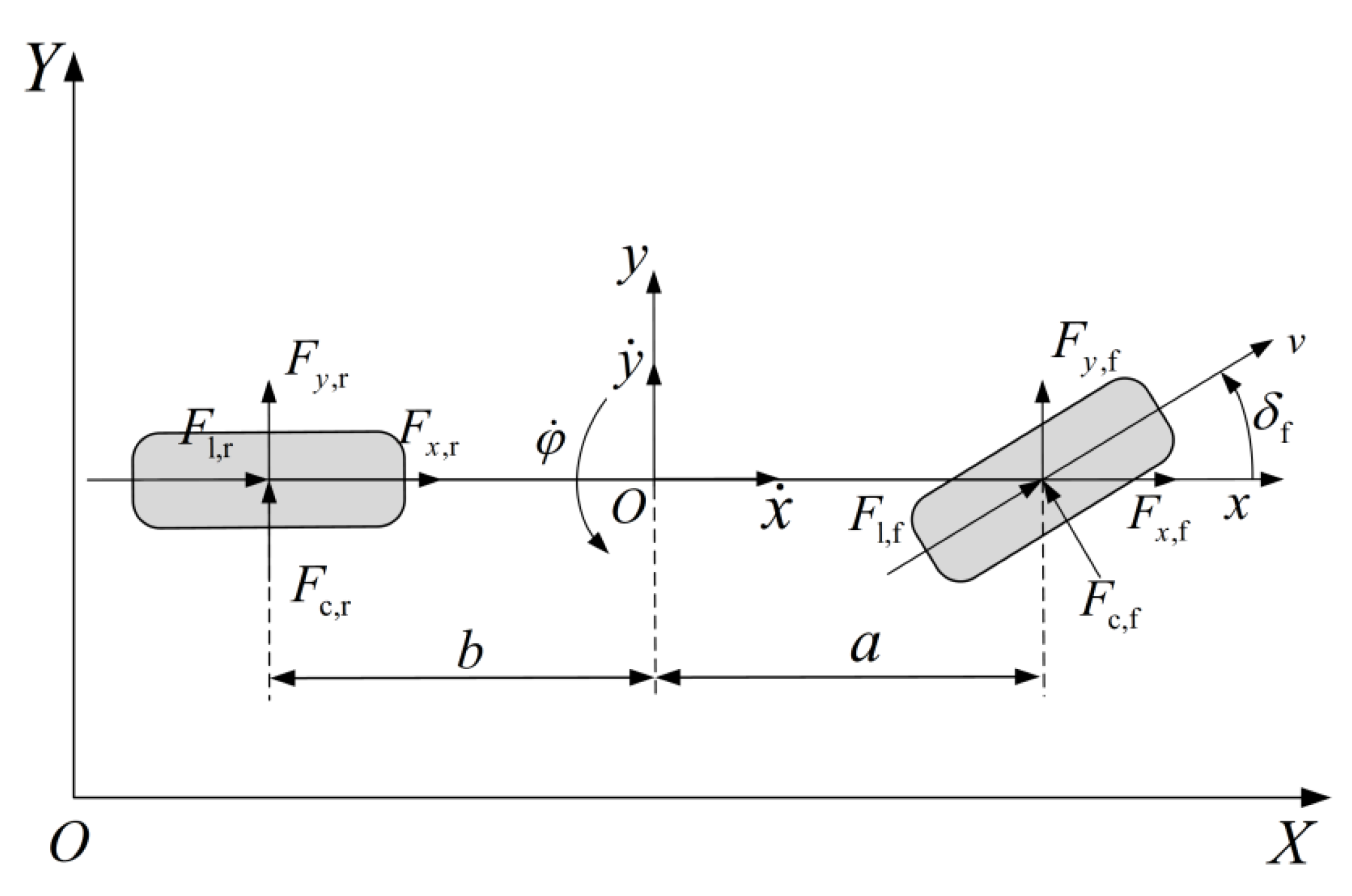
2.1. Vehicle Dynamics Modeling

The three-degree-of-freedom vehicle dynamics model is capable of precisely capturing the lateral, longitudinal and yaw dynamic characteristics exhibited during the path tracking process of an intelligent vehicle. In order to investigate the path tracking control of front wheel steering vehicles under varying road conditions, a simplified three-degree-of-freedom vehicle dynamics model is established in this section to serve as the MPC prediction model, as illustrated in Figure 1. In the diagram, $OXY$ is the geodetic inertial coordinate system; $oxy$ is the vehicle coordinate system; $a$, $b$ is the distance from the front and rear axles of the vehicle to the center of mass; $F_{x,\mathrm{f}}$, $F_{x,\mathrm{r}}$ denote the forces acting along the x-axis on the front and rear wheels; $F_{y,\mathrm{f}}$, $F_{x,\mathrm{r}}$ denote the forces acting along the y-axis on the front and rear wheels; $F_{l,\mathrm{f}}$, $F_{l,\mathrm{r}}$ denote the longitudinal forces experienced by the front and rear wheels; $F_{c,\mathrm{f}}$, $F_{c,\mathrm{r}}$ denote the lateral forces acting on the front and rear wheels; ${\delta }_{\mathrm{f}}$ is the steering angle of the front wheel; $\dot{x}$, $\dot{y}$ are the longitudinal and transverse speeds of the vehicle, respectively; $\dot{\phi }$ is the yaw rate of the vehicle.

According to the literature [32], the expression of a three-degree-of-freedom vehicle dynamics non-linear model based on a linear tire model can be expressed as

$$\left\{\begin{array}{l}\ddot{y}={\displaystyle \frac{2}{m}}\left[C_{c,\mathrm{r}}{\displaystyle \frac{b\dot{\phi }-\dot{y}}{\dot{x}}}+C_{l,\mathrm{f}}{S}_{\mathrm{f}}{\delta }_{\mathrm{f}}+C_{c,\mathrm{f}}\left({\delta }_{\mathrm{f}}-{\displaystyle \frac{\dot{y}+a\dot{\phi }}{\dot{x}}}\right)\right]-\stackrel{.}{x\dot{\phi }}\\ \ddot{x}={\displaystyle \frac{2}{m}}\left[C_{l,\mathrm{r}}{S}_{\mathrm{r}}+C_{l,\mathrm{f}}{S}_{\mathrm{f}}-C_{c,\mathrm{f}}\left({\delta }_{\mathrm{f}}-{\displaystyle \frac{\dot{y}+a\dot{\phi }}{\dot{x}}}\right){\delta }_{\mathrm{f}}\right]+\dot{y}\dot{\phi }\\ \ddot{\phi }={\displaystyle \frac{2a}{I_z}}\left[C_{l,\mathrm{f}}{S}_{\mathrm{f}}{\delta }_{\mathrm{f}}+C_{c,\mathrm{f}}\left({\delta }_{\mathrm{f}}-{\displaystyle \frac{\dot{y}+a\dot{\phi }}{\dot{x}}}\right)\right]-{\displaystyle \frac{2b}{I_z}}{C}_{c,\mathrm{r}}{\displaystyle \frac{b\dot{\phi }-\dot{y}}{\dot{x}}}\\ \dot{y}=\dot{x}\sin \phi +\dot{y}\cos \phi \hspace{1em}\hspace{1em}\dot{X}=\dot{x}\cos \phi -\dot{y}\sin \phi \end{array}\right.$$

(1)

where $m$ is the vehicle mass; $\ddot{x}$, $\ddot{y}$ are the longitudinal and transverse acceleration of the vehicle, respectively; $\dot{X}$, $\dot{Y}$ are, respectively, the longitudinal and lateral speeds of the vehicle in the global coordinate system; $\phi$ is the yaw angle of the vehicle; $\ddot{\phi }$ is the yaw rate acceleration; $I_z$ is the moment of inertia of the vehicle around the z-axis; $C_{l,\mathrm{f}}$, $C_{l,\mathrm{r}}$ are the longitudinal stiffness of front and rear wheels; $C_{c,\mathrm{f}}$, $C_{c,\mathrm{r}}$ are the lateral stiffness of front and rear wheels; $S_{\mathrm{f}}$, $S_{\mathrm{r}}$ are the slip ratio of front and rear wheels. The test vehicle parameters are shown in

Table 1. Test vehicle parameters.

Parameter/Unit	Value
Full mass of vehicle/m (kg)	1723
Distance from centroid to front axle/a (m)	1.232
Distance from centroid to rear axle/b (m)	1.468
Moment of inertia about Z-axis/Iz (kg·m2)	4175
Front wheel lateral stiffness/Cc,f (N·rad−1)	66,900
Rear wheel lateral stiffness/Cc,r (N·rad−1)	62,700

.

2.2. Model Linearization and Prediction Equation

Convert Equation (1) into the state-space representation to derive the vehicle control system model at any time point t:

$$\dot{\xi }(t)=f\left(\xi (t), \mathit{u}(t)\right), \mathit{y}(t)=\mathit{C}\mathit{\xi }(t)$$

(2)

Let $\xi ={\left[\dot{y},\dot{x},\phi ,\dot{\phi },Y,X\right]}^T$ be selected as the system state variable, the front wheel angle $\mathit{u}={\delta }_{\mathrm{f}}$ as the system control input, $\mathit{y}(t)={\left[\phi ,Y\right]}^T$ as the system output quantity, C as the output matrix, $\mathit{C}=\left[\begin{array}{cccccc}0\hfill & 0\hfill & 1\hfill & 0\hfill & 0\hfill & 0\hfill \\ 0\hfill & 0\hfill & 0\hfill & 0\hfill & 1\hfill & 0\hfill \end{array}\right]$, and let f (t) denote the mapping relationship.

When operating at high speeds, a vehicle necessitates a controller with high real-time capabilities, which the previously derived non-linear model finds challenging to fulfill. Consequently, Equation (2) undergoes linearization to yield a linear time-varying state equation:

$$\dot{\mathit{\xi }}=\mathit{A}(t)\mathit{\xi }(t)+\mathit{B}(t)\mathit{u}(t)$$

(3)

where $\mathit{A}(t)$ and $\mathit{B}(t)$ are the Jacobi matrix of $\mathit{\xi }$ and $\mathit{u}$ corresponding to the state equation, respectively.

$$\mathit{A}(t)=\left[\begin{array}{cccccc}\hfill {\displaystyle \frac{\partial f_{\dot{y}}}{\partial \dot{y}}}\hfill & \hfill {\displaystyle \frac{\partial f_{\dot{y}}}{\partial \dot{x}}}\hfill & \hfill 0\hfill & \hfill {\displaystyle \frac{\partial f_{\dot{y}}}{\partial \dot{\phi }}}\hfill & \hfill 0\hfill & \hfill 0\hfill \\ \hfill {\displaystyle \frac{\partial f_{\dot{x}}}{\partial \dot{y}}}\hfill & \hfill {\displaystyle \frac{\partial f_{\dot{x}}}{\partial \dot{x}}}\hfill & \hfill 0\hfill & \hfill {\displaystyle \frac{\partial f_{\dot{x}}}{\partial \dot{\phi }}}\hfill & \hfill 0\hfill & \hfill 0\hfill \\ \hfill 0\hfill & \hfill 0\hfill & \hfill 0\hfill & \hfill 1\hfill & \hfill 0\hfill & \hfill 0\hfill \\ \hfill {\displaystyle \frac{\partial f_{\dot{\phi }}}{\partial \dot{y}}}\hfill & \hfill {\displaystyle \frac{\partial f_{\dot{\phi }}}{\partial \dot{x}}}\hfill & \hfill 0\hfill & \hfill {\displaystyle \frac{\partial f_{\dot{\phi }}}{\partial \dot{\phi }}}\hfill & \hfill 0\hfill & \hfill 0\hfill \\ \hfill \cos \phi \hfill & \hfill \sin \phi \hfill & \hfill \dot{x}\cos \phi -\dot{y}\sin \phi \hfill & \hfill 0\hfill & \hfill 0\hfill & \hfill 0\hfill \\ \hfill -\sin \phi \hfill & \hfill \cos \phi \hfill & \hfill -\dot{x}\sin \phi -\dot{y}\cos \phi \hfill & \hfill 0\hfill & \hfill 0\hfill & \hfill 0\hfill \end{array}\right]$$

In $\mathit{A}(t)$, ${\displaystyle \frac{\partial f_{\dot{y}}}{\partial \dot{y}}}=-{\displaystyle \frac{2(C_{c,\mathrm{f}}+C_{c,\mathrm{r}})}{m\dot{x}}}$, ${\displaystyle \frac{\partial f_{\dot{y}}}{\partial \dot{x}}}=-\dot{\phi }+{\displaystyle \frac{C_{c,\mathrm{f}}+C_{c,\mathrm{r}}}{m{\dot{x}}^2}}\dot{y}-{\displaystyle \frac{C_{c,\mathrm{r}}b-C_{c,\mathrm{f}}a}{m{\dot{x}}^2}}\dot{\phi }$,

${\displaystyle \frac{\partial f_{\dot{y}}}{\partial \dot{\phi }}}=-\dot{x}+{\displaystyle \frac{2(C_{c,\mathrm{r}}b+C_{c,\mathrm{f}}a)}{m\dot{x}}}$, ${\displaystyle \frac{\partial f_{\dot{x}}}{\partial \dot{y}}}=\dot{\phi }-{\displaystyle \frac{2C_{c,\mathrm{f}}{\delta }_{\mathrm{f}}}{m\dot{x}}}$, ${\displaystyle \frac{\partial f_{\dot{x}}}{\partial \dot{x}}}={\displaystyle \frac{2C_{c,\mathrm{f}}{\delta }_{\mathrm{f}}(\dot{y}+a\dot{\phi })}{m{\dot{x}}^2}}$,

${\displaystyle \frac{\partial f_{\dot{x}}}{\partial \dot{\phi }}}=\dot{y}-{\displaystyle \frac{2a{C}_{c,\mathrm{f}}{\delta }_{\mathrm{f}}}{m\dot{x}}}$, ${\displaystyle \frac{\partial f_{\dot{\phi }}}{\partial \dot{y}}}={\displaystyle \frac{2(C_{c,\mathrm{r}}b-C_{c,\mathrm{f}}a)}{I_z\dot{x}}}$,

${\displaystyle \frac{\partial f_{\dot{\phi }}}{\partial \dot{x}}}=-{\displaystyle \frac{C_{c,\mathrm{r}}b-C_{c,\mathrm{f}}a}{I_z{\dot{x}}^2}}\dot{y}+{\displaystyle \frac{C_{c,\mathrm{f}}{a}^2+C_{c,\mathrm{r}}{b}^2}{I_z{\dot{x}}^2}}\dot{\phi }$, ${\displaystyle \frac{\partial f_{\dot{\phi }}}{\partial \dot{\phi }}}=-{\displaystyle \frac{2(C_{c,\mathrm{f}}{a}^2+C_{c,\mathrm{r}}{b}^2)}{I_z\dot{x}}}$.

$$\mathit{B}(t)={\left.{\displaystyle \frac{\delta f}{\delta u}}\right|}_{\begin{array}{l}\xi =\xi (t)\\ u=\mathit{u}(t)\end{array}}={\left[\begin{array}{cccccc}{\displaystyle \frac{2C_{\mathrm{c},\mathrm{f}}}{m}}\hfill & {\displaystyle \frac{2C_{c,\mathrm{f}}(2{\delta }_f-\frac{{\dot{y}}_t+a{\dot{\phi }}_t}{{\dot{x}}_t})}{m}}\hfill & 0\hfill & {\displaystyle \frac{2C_{c,\mathrm{f}}a}{I_z}}\hfill & 0\hfill & 0\hfill \end{array}\right]}^T$$

The linear discrete state-space representation can be acquired by discretizing Equation (3) using the forward Euler method:

$$\left\{\begin{array}{l}\Delta \mathit{\xi }(k+1)=\mathit{A}(k)\Delta \mathit{\xi }(k)+\mathit{B}(k)\Delta \mathit{u}(k)\\ \mathit{y}(k)=\mathit{C}\Delta \mathit{\xi }(k)\end{array}\right.$$

(4)

where $\mathit{A}(k)=\mathit{I}+T\mathit{A}(t)$, $\mathit{B}(k)=T\mathit{B}(t)$, I denote the identity matrix, and T represents the sampling period.

Formulate a prediction equation to calculate the current state vector $\xi (k)$ and the control input sequence $\Delta \mathit{U}(k)$ over the control time horizon, thereby obtaining the future system output:

$$\mathit{\xi }(k | t)=\left[\begin{array}{c}\mathit{\xi }(k | t)\\ u(k-1 | t)\end{array}\right]$$

(5)

By integrating Formulae (4) and (5), a novel state-space expression is derived:

$$\left\{\begin{array}{l}\mathit{\xi }(k+1 | t)=\tilde{A}(k)\mathit{\xi }(k | \mathrm{t})+\tilde{B}(k)\Delta \mathit{u}(k | \mathrm{t})\\ \mathit{y}(k | \mathrm{t})=\tilde{C}(k)\mathit{\xi }(k | \mathrm{t})\end{array}\right.$$

(6)

where $\tilde{A}(k)=\left[\begin{array}{cc}\mathit{A}(k)& \mathit{B}(k)\\ 0& I\end{array}\right]$, $\tilde{B}(k)=\left[\begin{array}{c}\mathit{B}(k)\\ I\end{array}\right]$, $\tilde{C}(k)=\left[\begin{array}{cc}C& 0_{2\times 1}\end{array}\right]$, $\Delta \mathit{u}(k | \mathrm{t})=\mathit{u}(k)-\mathit{u}(k-1)$.

Define the system output and input at time k as follows:

$$\mathit{Y}(k+1 \mid k)=\left[\begin{array}{c}\mathit{y}(k+1 \mid k)\\ \mathit{y}(k+2 \mid k)\\ \cdots \\ \mathit{y}\left(k+N_{\mathrm{c}} \mid k\right)\\ \cdots \\ \mathit{y}\left(k+N_{\mathrm{p}} \mid k\right)\end{array}\right], \Delta \mathit{U}(k)=\left[\begin{array}{c}\Delta \mathit{u}(k \mid k)\\ \Delta \mathit{u}(k+1 \mid k)\\ \cdots \\ \Delta \mathit{u}\left(k+N_{\mathrm{c}} \mid k\right)\end{array}\right]$$

(7)

where $N_{\mathrm{p}}$ is the prediction horizon, $N_{\mathrm{c}}$ is the control horizon, $N_{\mathrm{p}}>N_{\mathrm{c}}$.

By substituting Equation (7) into Equation (6), the expression of the prediction equation of the system can be expressed as

$$\mathit{Y}(k+1 \mid k)=\mathit{\psi }\mathit{\xi }(k)+\mathit{\Theta }\Delta \mathit{U}(k)$$

(8)

where $\mathit{\Theta }=\left[\begin{array}{cccc}C\tilde{B}(k)& 0& 0& 0\\ C\tilde{A}(k)\tilde{B}(k)& C\tilde{B}(k)& 0& 0\\ \cdots & \cdots & \ddots & \cdots \\ \begin{array}{c}C\tilde{A}{(k)}^{N_{\mathrm{c}}-1}\tilde{B}(k)\\ \begin{array}{c}C\tilde{A}{(k)}^{N_{\mathrm{c}}}\tilde{B}(k)\\ ⋮\\ C\tilde{A}{(k)}^{N_{\mathrm{p}}-1}\tilde{B}(k)\end{array}\end{array}& \begin{array}{c}\begin{array}{c}C\tilde{A}{(k)}^{N_{\mathrm{c}}-2}\tilde{B}(k)\\ C\tilde{A}{(k)}^{N_{\mathrm{c}}-1}\tilde{B}(k)\\ ⋮\end{array}\\ C\tilde{A}{(k)}^{N_{\mathrm{p}}-2}\tilde{B}(k)\end{array}& \begin{array}{c}\cdots \\ \begin{array}{c}\cdots \\ \ddots \\ \cdots \end{array}\end{array}& \begin{array}{c}C\tilde{B}(k)\\ \begin{array}{c}C\tilde{A}(k)\tilde{B}(k)\\ ⋮\\ C\tilde{A}{(k)}^{N_{\mathrm{p}}-N_{\mathrm{c}}-1}\tilde{B}(k)\end{array}\end{array}\end{array}\right]$, $\mathit{\psi }=\left[\begin{array}{c}C\tilde{A}(k)\\ C\tilde{A}{(k)}^2\\ \begin{array}{c}⋮\\ C\tilde{A}{(k)}^{N_{\mathrm{c}}}\\ ⋮\end{array}\\ C\tilde{A}{(k)}^{N_{\mathrm{p}}}\end{array}\right]$.

The primary objective of the linearization approach is to enable real-time computation capabilities for model predictive control (MPC) implementation, which is a prevalent practice in automotive control systems. This necessity arises from several critical factors: the stringent timing requirements that sampling rates must adhere to, the constrained computational resources of controller hardware and the imperative for predictions to be completed within fixed control cycles. The linearized model in this paper adheres to well-established procedures within the vehicle dynamics control literature, as evidenced by the references cited in the work.

The reference trajectory is initially generated by the path planning module, which provides a series of waypoints (X_ref, Y_ref) based on the vehicle’s global positioning and road geometry information. These waypoints encompass the desired lateral positions, heading angles and curvature details. Based on the vehicle’s current speed and the sampling period, the waypoints in global coordinates are discretized into time-series data y_ref(k), ensuring that the reference trajectory can be dynamically updated to align with the vehicle’s motion state. The curvature of the reference path is calculated and integrated into Equation (6) to account for variable curvature conditions. This enables the MPC controller to anticipate upcoming changes in the road geometry and adjust the control inputs accordingly.

3. MPC Controller Design Based on Stability Boundary

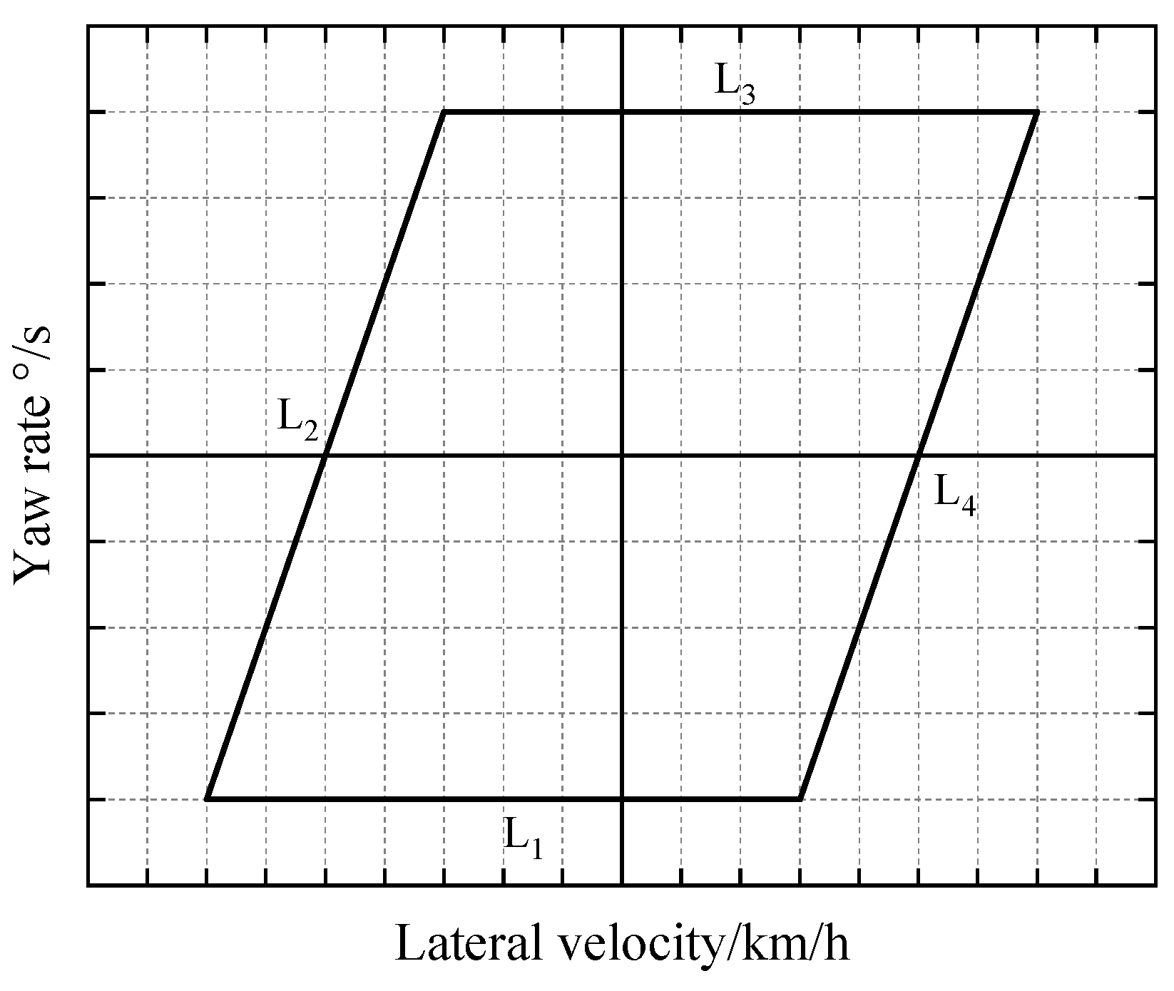
3.1. Vehicle Stability Boundary

In order to ensure the stability and precision of path tracking of the MPC controller based on the dynamic model, precision constraints are incorporated into the controller design. The yaw stability of vehicles under extreme conditions holds particular significance. Currently, the phase plane method is frequently employed to analyze the yaw stability boundary of vehicles. Specifically, the phase plane method based on yaw rate/lateral velocity can accurately depict the yaw motion characteristics of the vehicle and the constraints imposed on the tire’s sideslip angle, yielding promising results in real vehicle testing. Consequently, based on this method, the yaw stability criterion for vehicles with front wheel steering is derived, followed by the establishment of adaptive constraint conditions.

According to the vehicle yaw dynamic model (1) under the small angle assumption

$$\left\{\begin{array}{l}\dot{y}=-\dot{\phi }\dot{x}+{\displaystyle \frac{2(F_{y,\mathrm{f}}+F_{y,\mathrm{r}})}{m}}\\ \ddot{\phi }={\displaystyle \frac{2(a{F}_{y,\mathrm{f}}-b{F}_{y,\mathrm{r}})}{I_z}}\end{array}\right.$$

(9)

Given the rear axle sideslip poses a greater risk during vehicle yaw instability [33], this paper examines a scenario where the rear wheel side deflection angle attains its steady-state limit value.

The calculation formulae for the front and rear wheel slip angles are as follows:

$$\left\{\begin{array}{c}{\alpha }_{\mathrm{f}}={\displaystyle \frac{\dot{y}+a\dot{\phi }}{\dot{x}}}-{\delta }_{\mathrm{f}}\hfill \\ {\alpha }_{\mathrm{r}}={\displaystyle \frac{\dot{y}-b\dot{\phi }}{\dot{x}}}\hfill \end{array}\right.$$

The simplified expressions of the lateral forces acting on the front and rear wheels of a vehicle are as follows:

$$\left\{\begin{array}{c}{F}_{c,\mathrm{f}}=C_{c,\mathrm{f}}({\displaystyle \frac{\dot{y}+a\dot{\phi }}{\dot{x}}}-{\delta }_{\mathrm{f}})\hfill \\ F_{c,\mathrm{r}}=C_{c,\mathrm{r}}{\displaystyle \frac{\dot{y}-b\dot{\phi }}{\dot{x}}}\hfill \end{array}\right.$$

During the driving process of a vehicle, there are the following transformation relationships between the forces acting on the front and rear wheels along the x-axis and y-axis directions and the tire lateral forces:

$$\left\{\begin{array}{c}{F}_{y,\mathrm{f}}=F_{l,\mathrm{f}}\sin {\delta }_{\mathrm{f}}+F_{c,\mathrm{f}}\cos {\delta }_{\mathrm{f}}\hfill \\ F_{y,\mathrm{r}}=F_{l,\mathrm{r}}\sin {\delta }_{\mathrm{r}}+F_{c,\mathrm{r}}\cos {\delta }_{\mathrm{r}}\hfill \end{array}\right.$$

Thus, by combining Equations (1) and (9), the maximum control law of the yaw rate at any k time can be obtained:

$${\dot{\phi }}_{\mathrm{ss},\max }(k)={\displaystyle \frac{C_{c,\mathrm{r}}{\alpha }_{\mathrm{r},\max }(1+\frac{b}{a})}{m\dot{x}(k)}}$$

(10)

Here, ${\alpha }_{\mathrm{r},\max }$ represents the steady-state limit value of the sideslip angle for the rear wheel when an impending sideslip occurs. According to the literature [34], when the tire sideslip angle is ≤5°, the lateral force and sideslip angle exhibit an approximately linear relationship. To ensure good driving stability of the vehicle on low-adhesion roads, this paper further restricts the tire sideslip angle to $-2.5°⩽{\alpha }_{\mathrm{f}}⩽2.5°$.

Consequently, the constraint relationship for the yaw rate is as follows:

$$-{\displaystyle \frac{C_{\mathrm{c},\mathrm{r}}{\alpha }_{\mathrm{r},\max }(1+\frac{b}{a})}{m\dot{x}(k)}}⩽{\dot{\phi }}_{\mathrm{ss}}(k)⩽{\displaystyle \frac{C_{\mathrm{c},\mathrm{r}}{\alpha }_{\mathrm{r},\max }(1+\frac{b}{a})}{m\dot{x}(k)}}$$

(11)

The restraint relationship of vehicle lateral speed meets

$$-{\alpha }_{\mathrm{r},\max }⩽{\displaystyle \frac{\dot{y}-b\dot{\phi }}{\dot{x}(k)}}⩽{\alpha }_{\mathrm{r},\max }$$

(12)

Based on the aforementioned equations, the stability boundary constraint condition derived from the relationship between the yaw rate and lateral velocity can be reformulated into the subsequent matrix inequality form:

$$-{\mathit{G}}_{\mathrm{sh}}(k)⩽{\mathit{H}}_{\mathrm{sh}}(k)\xi (k)⩽{\mathit{G}}_{\mathrm{sh}}(k)$$

(13)

Here, ${\mathit{G}}_{\mathrm{sh}}(k)=\left[\begin{array}{c}{\alpha }_{\mathrm{r},\max }\\ {\displaystyle \frac{C_{\mathrm{c},\mathrm{r}}{\alpha }_{\mathrm{r},\max }(1+\frac{b}{a})}{m\dot{x}(k)}}\end{array}\right]$, ${\mathit{H}}_{\mathrm{sh}}(k)=\left[\begin{array}{cccccc}{\displaystyle \frac{1}{\dot{x}(k)}}& -{\displaystyle \frac{b}{\dot{x}(k)}}& 0& 0& 0& 0\\ 0& 1& {\displaystyle \frac{g}{\dot{x}(k)}}& 0& 0& 0\end{array}\right]$, $\xi (k)$ represents the status of the vehicle at the k-th time.

In the phase plane of the yaw rate/lateral velocity, a closed stability boundary can be constructed by employing Equations (11) and (12), as illustrated in Figure 2. The extent of the boundary is influenced by the longitudinal speed of the vehicle and the side deflection angle of the rear wheel. Specifically, the stability boundaries L₁ and L₃ are constrained by Equation (11), whereas the stability boundaries L₂ and L₄ are subject to the constraints imposed by Equation (12). When the vehicle’s state variables lie within the stability boundary, driving stability can be ensured.

Furthermore, it is worth noting that when the vehicle tire operates within the non-linear region for a brief duration, it does not inevitably result in vehicle instability. In order to avoid overly restricting the solution space of the controller, a relaxation factor can be introduced into Equation (13), leading to its revised formulation as follows:

$$-{\mathit{G}}_{\mathrm{sh}}(k)-{\mathit{S}}_{\mathrm{sh}}(k)⩽{\mathit{H}}_{\mathrm{sh}}(k)\xi (k)⩽{\mathit{G}}_{\mathrm{sh}}(k)+{\mathit{S}}_{\mathrm{sh}}(k)$$

(14)

In this context, ${\mathit{S}}_{\mathrm{sh}}(k)={\left[\begin{array}{cc}{\alpha }_{\mathrm{r},\mathrm{sh}}& {\dot{\phi }}_{\mathrm{sh}}\end{array}\right]}^T$ represents the relaxation factor vector pertaining to the stability boundary constraint; ${\alpha }_{\mathrm{r},\mathrm{sh}}$ denotes the relaxation measure for the rear wheel side deflection constraint; and ${\dot{\phi }}_{\mathrm{sh}}$ signifies the relaxation parameter for the yaw rate constraint.

3.2. Solve MPC Controller

In the design process of MPC controllers, in addition to incorporating appropriate constraints, it is also necessary to design a suitable objective function. Given that a vehicle dynamics model is employed in this study, and numerous constraints are imposed, there may be instances of infeasible solutions during the computation process. To reduce computational complexity and enhance system operational efficiency, a slack variable is incorporated into the objective function of the MPC controller [35].

The objective function formulated in this study is expressed as follows:

$$J(\mathit{\xi }(t),\mathit{u}(t-1),\Delta \mathit{U}(t))={\displaystyle \mathbf{\sum }_{i=1}^{N_{\mathrm{p}}}\parallel \mathit{y}(}t+i \mid t)-{\mathit{y}}_{\mathrm{ref}}(t+i \mid t){\parallel }_{\mathit{Q}}^2+{\displaystyle \sum _{i=1}^{N_{\mathrm{c}}-1}\parallel \Delta \mathit{u}(}t+i \mid t){\parallel }_{\mathit{R}}^2+\rho {\epsilon }^2$$

(15)

where Q and R are the weighting matrices; $\rho$ is the weight coefficient; and $\epsilon$ is the relaxation factor. The first term of the objective function represents the discrepancy between the anticipated path and the system output. The second term accounts for the control increment of the system, while the third term serves to enable the controller to adjust the constraint range. The entire objective function is meticulously crafted to guarantee the accuracy, stability and viability of the controller during the path tracking procedure.

The deviation between the predicted outputs (Y(k)) and the reference trajectory (y_ref(k)) is embedded into Equation (15), enabling the controller to minimize tracking errors while satisfying stability constraints.

The controller cannot directly solve the path tracking optimization problem represented by Formula (15). Instead, it is necessary to transform this path tracking optimization problem into a quadratic programming problem that can be directly solved by the controller.

During the optimization process of the objective function, since the variables to be solved are control increments within the control horizon, the established constraints need to be converted into forms involving control increments or the product of control increments and a transformation matrix.

The following relationship exists between the control variable and the control increment of the system:

$$\mathit{u}(t+k)=\mathit{u}(t+k-1)+\Delta \mathit{u}(t+k)$$

Therefore, it is set as follows:

$$\mathit{U}(t)={\mathit{I}}_{N_{\mathrm{c}}}\otimes \mathit{u}(k-1)$$

$$\mathit{A}=\left(\begin{array}{ccccc}1\hfill & 0\hfill & \cdots \hfill & 0\hfill & 0\hfill \\ 1\hfill & 1\hfill & 0\hfill & \cdots \hfill & 0\hfill \\ 1\hfill & 1\hfill & 1\hfill & \ddots \hfill & ⋮\hfill \\ ⋮\hfill & ⋮\hfill & ⋮\hfill & \ddots \hfill & 0\hfill \\ 1\hfill & 1\hfill & 1\hfill & \cdots \hfill & 1\hfill \end{array}\right)\otimes {\mathit{I}}_{\mathrm{m}}$$

In the formula, ${\mathit{I}}_{N_c}$ is a column vector with ${\mathit{N}}_{\mathrm{c}}$ rows; ${\mathit{I}}_{\mathrm{m}}$ is an identity matrix of dimension m; $\otimes$ denotes the Kronecker product of two matrices; and $\mathit{u}(k-1)$ represents the actual control variable in the previous control horizon.

The formula can be derived as follows:

$${\mathit{U}}_{\min }\le A\Delta \mathit{U}(t)+\mathit{U}(t)\le {\mathit{U}}_{\max }$$

By substituting Equation (8) into the objective function expressed in Equation (15), the output deviation within the prediction horizon is obtained as follows:

$$\left\{\begin{array}{c}{\mathit{Y}}_{\mathrm{ref}}(t)={\left[\begin{array}{ccc}{y}_{\mathrm{ref}}(t+1\left|t\right.)& \cdots & y_{\mathrm{ref}}(t+N_{\mathrm{p}}\left|t\right.)\end{array}\right]}^{\mathrm{T}}\hfill \\ \mathit{E}(t)=\mathit{\psi }\mathit{\xi }(t)+\mathit{\Theta }\Delta \mathit{U}(t)-{\mathit{Y}}_{\mathrm{ref}}(t)\hfill \end{array}\right.$$

By synthesizing the above expressions, the objective function is transformed into a standard quadratic form.

$$J(\mathit{\xi }(t),\mathit{u}(t-1),\Delta \mathit{U}(t))={\left[\Delta \mathit{U}{(t)}^T, \epsilon \right]}^T{\mathit{H}}_{\mathrm{t}}{\left[\Delta \mathit{U}{(t)}^T, \epsilon \right]}^T+{\mathit{G}}_{\mathrm{t}}{\left[\Delta \mathit{U}{(t)}^T, \epsilon \right]}^T+{\mathit{P}}_{\mathrm{t}}$$

where ${\mathit{H}}_{\mathrm{t}}=\left[\begin{array}{cc}\mathit{\Theta }{\mathit{Q}}_Q\mathit{\Theta }+{\mathit{R}}_R& 0\\ 0& \rho \end{array}\right]$, ${\mathit{G}}_{\mathrm{t}}=\left[\begin{array}{cc}2\mathit{E}{(t)}^T{\mathit{Q}}_Q\mathit{\Theta }& 0\end{array}\right]$, ${\mathit{P}}_{\mathrm{t}}=\mathit{E}{(t)}^T{\mathit{Q}}_Q\mathit{E}(t)$, ${\mathit{Q}}_Q={\mathit{I}}_{{\mathit{N}}_{\mathrm{p}}}\otimes \mathit{Q}$, ${\mathit{R}}_R={\mathit{I}}_{N_{\mathrm{p}}}\otimes \mathit{R}$.

The constraint conditions and objective functions are incorporated into the solving process of quadratic programming to obtain Equation (16). Within each sampling period, the path tracking controller is tasked with solving the subsequent multi-objective optimization problems:

$$\left\{\begin{array}{c}\min J(\xi (t),\mathit{u}(t-1),\Delta \mathit{U}(t),\epsilon )\hfill \\ \Delta {\mathit{U}}_{\min }⩽\Delta \mathit{U}(t)⩽\Delta {\mathit{U}}_{\max }\hfill \\ {\mathit{U}}_{\min }⩽\mathit{A}\Delta \mathit{U}(t)+\mathit{U}(t)⩽{\mathit{U}}_{\max }\hfill \\ {\mathit{y}}_{\mathrm{h},\min }⩽{\mathit{y}}_{\mathrm{h}}⩽{\mathit{y}}_{\mathrm{h},\max }\hfill \\ {\mathit{y}}_{\mathrm{s},\min }-\epsilon ⩽ {\mathit{y}}_{\mathrm{s}}⩽{\mathit{y}}_{\mathrm{s},\max }+\epsilon \hfill \end{array}\right.$$

(16)

where U_max and U_min are the maximum and minimum values of the control quantity, respectively; ${\mathit{y}}_{\mathrm{h}}$, ${\mathit{y}}_{\mathrm{s}}$ are the hard constraint output and the soft constraint output, respectively. ${\mathit{y}}_{\mathrm{h},\min }$, ${\mathit{y}}_{\mathrm{h},\max }$, ${\mathit{y}}_{\mathrm{s},\min }$, ${\mathit{y}}_{\mathrm{s},\max }$ are the limit values of the hard constraint output and soft constraint output, respectively.

The system obtains the control increment sequence through QP solution in each control time domain:

$$\Delta \mathit{U}{(t)}^{*}={\left[\Delta {\mathit{u}}_t^{*},\Delta {\mathit{u}}_{t+1}^{*},\cdots ,{\Delta {\mathit{u}}_{t+N_{c-1}}}^{*}\right]}^{\mathrm{T}}$$

(17)

By inputting the first element in Equation (17) into the system as the actual control increment, it can be obtained that

$$\mathit{u}(t)=\mathit{u}(t-1)+\Delta {\mathit{u}}_t^{*}$$

(18)

Upon entering the subsequent control time domain, the system perpetually iterates through the aforementioned process, thereby enabling closed-loop tracking of the reference path. The devised MPC control algorithm is implemented via an S-function, and an intelligent vehicle path tracking controller is established on the CarSim/Simulink co-simulation platform. Certain controller parameters are detailed in

Table 2. The controller parameters.

Parameter/Unit	Value
Sampling period T	0.05
Weighting matrix Q	Diag [200, 100, 100]
Weighting matrix R	[5 × 104]
Weight coefficient ρ	1000

.

The following is an explanation for the determination of the controller parameters in Table 2.

(1)

Determination of Weighting Matrices Q and R:

Q Matrix (State Weighting): The relative importance of lateral deviation, heading deviation and yaw rate in path tracking was analyzed. Initial values were referenced from classical MPC literature, followed by iterative tuning via CarSim/Simulink co-simulation under typical conditions (e.g., double lane change, serpentine curves). The final selection, Q = diag [200, 100, 100], prioritizes lateral tracking accuracy.

R Matrix (Control Input Weighting): To prevent abrupt front wheel steering, a high weight (R = [5 × 10⁴]) was set based on vehicle dynamic stability constraints, ensuring smooth control inputs.

(2)

Relaxation Factor Weight (ρ):

To balance constraint violations and optimization objectives, ρ = 1000 was selected through genetic algorithm testing across multiple scenarios, ensuring solver feasibility even when tire slip angles approach non-linear regions.

(3)

Sampling Period (T):

Considering both real-time performance (computational load) and control precision, T = 0.05 s was chosen based on vehicle dynamics time constants (0.05~0.1 s) and hardware capabilities.

4. Condition-Adaptive MPC Controller

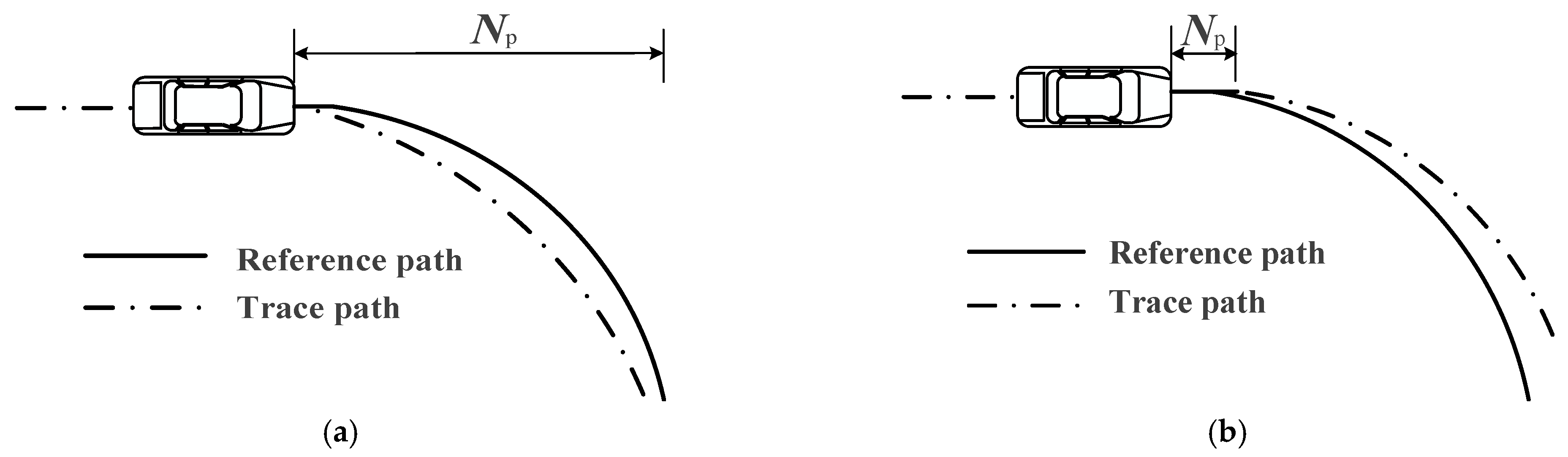
4.1. Factors Affecting MPC Path Tracking

In the MPC controller, the prediction horizon N_p indicates the number of future time steps the system predicts, and the control horizon N_c represents the number of groups of control increments the system solves in a control cycle. As shown in Figure 3, when N_p is large, the controller can predict a longer period, but the weight assigned to tracking errors far from the current position will be greater, leading to an increase in the cumulative error and heightened complexity in controller solution. When N_p is small, the controller has a lower calculation burden, enabling faster system response and higher real-time performance. However, the predicted distance is too short, which reduces system responsiveness to the future. Under the constraint of the controller on the front wheel angle, the vehicle may fail to turn in time, leading to path tracking failure. When N_c increases, the sensitivity and accuracy of the controller will be improved, but this will increase the amount of calculation and reduce the real-time performance and stability of the system. When N_c decreases, the sensitivity and accuracy of the controller decrease, but the stability and real-time performance of the system will be improved.

Vehicle speed and road curvature are pivotal factors influencing MPC path tracking. During path tracking, the vehicle’s anticipated rotation angle varies in tandem with alterations in road curvature [36]. Given that the controller imposes limitations on steering angular velocity, the vehicle necessitates a certain duration to output the desired steering angle. As depicted in Figure 4, when the vehicle is moving at a slower speed, its turning radius is smaller; conversely, at higher speeds, the turning radius increases. In such scenarios, if the vehicle traverses a curve with significant curvature, a substantial tracking deviation may arise.

In summary, the tracking performance of the MPC is highly contingent upon its time domain parameters. Moreover, the optimal time domain parameters of the system are not static; they undergo changes in response to variations in the current road curvature and vehicle speed.

4.2. Division of Steady-State Steering Conditions

In order to enhance the tracking accuracy of the MPC algorithm across a range of vehicle speeds and varying curvature conditions, it is essential to incorporate feedback mechanisms involving longitudinal vehicle speed and road curvature radius into the MPC controller. This integration enables the analysis and matching of optimal control parameters, facilitating the achievement of adaptive control parameters that better align with real-time driving conditions. Consequently, the dynamic characteristics of intelligent vehicles are more accurately captured, thereby enabling precise path tracking even under complex driving scenarios. As a reference,

Table 3. Minimum road curvature radius corresponding to different design speeds.

Speed/km/h	20	30	40	60	80	100	120
Minimum radius of curvature (general value)/m	30	65	100	200	400	700	1000
Minimum radius of curvature (limit value)/m	15	30	60	125	250	400	650

presents the minimum road curvature radius corresponding to different design speeds, as outlined in the China National Highway Route Design Specification JTG D20-2017.

When a vehicle is in motion, its turning radius must not fall below the threshold value defined by the minimum road curvature radius corresponding to the design speed of the current road section. In accordance with the uniform design principle and the minimum road curvature radius stipulated by the design speed, 100 distinct groups of steady-state steering conditions were categorized, as illustrated in

Table 4. Division of steady-state steering conditions.

Speed/km/h	10	20	30	40	50	60	70	80	90	100
Radius of road curvature /m	6	15	30	60	90	125	185	250	320	400
	8	20	35	65	100	135	200	270	350	440
	10	25	40	70	110	145	215	290	380	480
	12	30	45	75	120	155	230	310	410	520
	14	35	50	80	130	165	245	330	440	560
	16	40	55	85	140	175	260	350	470	600
	18	45	60	90	150	185	275	370	500	640
	20	50	65	95	160	195	290	390	530	680
	22	55	70	100	170	205	305	410	560	720
	24	60	75	105	180	215	320	430	590	760

.

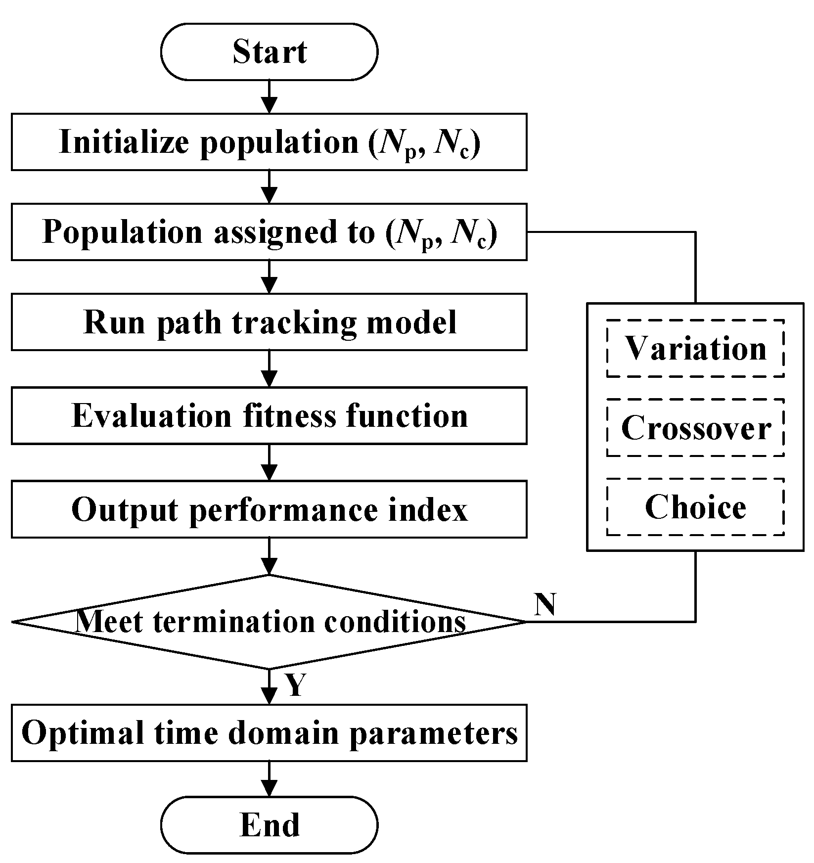
4.3. Solving Optimal Time Domain Parameter Combination Based on GA

Table 4 delineates numerous typical curve conditions (totaling 100 groups), rendering the enumeration method impractical for identifying the optimal solution. The genetic algorithm (GA) offers distinct advantages, including robust global search capabilities, rapid convergence speed and high search efficiency. Consequently, in this study, the genetic algorithm toolbox within MATLAB R2020b is employed to optimize the time domain parameters across various operational conditions.

The time domain parameter matrix of the MPC controller is determined as the optimization objective:

$$K_1=\left[\begin{array}{cc}{N}_{\mathrm{p}}& N_{\mathrm{c}}\end{array}\right]$$

(19)

To improve the optimization efficiency, set the prediction horizon value range N_p∈(0,40] and the control horizon value range N_c∈(0,20].

Since the dimensions of the lateral deviation and heading deviation of vehicle path tracking are inconsistent, they are normalized:

$$\left\{\begin{array}{l}{\overline{y}}_{\mathrm{e}}=1-2{\displaystyle \frac{y_{\mathrm{e}\max }-y_{\mathrm{e}}}{y_{\mathrm{e}\max }-y_{\mathrm{e}\min }}}\\ {\overline{\phi }}_{\mathrm{e}}=1-2{\displaystyle \frac{{\phi }_{\mathrm{e}\max }-{\phi }_{\mathrm{e}}}{{\phi }_{\mathrm{e}\max }-{\phi }_{\mathrm{e}\min }}}\end{array}\right.$$

(20)

where ${\overline{y}}_{\mathrm{e}}$ and ${\overline{\phi }}_{\mathrm{e}}$ are, respectively, the lateral deviation and heading deviation after the above treatment. $y_{\mathrm{e}\max }$ and $y_{\mathrm{e}\min }$ are, respectively, the maximum and minimum lateral deviation generated when tracking the target path. ${\phi }_{\mathrm{e}\max }$ and $y_{\mathrm{e}\min }$ are the maximum and minimum values of heading deviation, respectively.

Set the comprehensive deviation during vehicle path tracking as

$$e=\kappa {\overline{y}}_{\mathrm{e}}+(1-\kappa ){\overline{\phi }}_{\mathrm{e}}$$

(21)

where $\mathit{\kappa }$ denotes the deviation weight coefficient, which is assigned a value of 0.5 in this paper.

The fitness function for the genetic algorithm is designed by incorporating the time index and the squared error resulting from time multiplication [37]:

$$J={\displaystyle {\int }_{{\mathrm{t}}_1}^{{\mathrm{t}}_2}t} | e(t)|\mathrm{d}t$$

(22)

(1)

Optimization Problem Definition:

The performance function is explicitly defined in Equation (22) as the fitness function for GA optimization, combining the tracking accuracy and control effort. The search space boundaries for the time domain parameters are Np∈(0,40] and Nc∈(0,20]. The vehicle stability constraints in Equation (14) ensure that the yaw rate and lateral velocity remain within safe limits.

(2)

GA Configuration and Performance:

Parameters: Population size = 50, Generations = 20, Crossover probability = 0.5, Mutation probability = 0.1.

Performance: The optimized results in

Table 5. Optimal time domain parameter combination under various operating conditions.

Speed/km/h	10	20	30	40	50	60	70	80	90	100
Group 1	5.1	7.1	8.2	10.2	12.3	15.4	17.4	17.5	18.6	20.6
Group 2	5.1	7.1	8.2	10.2	12.3	16.4	17.4	18.5	19.6	20.7
Group 3	5.1	7.1	9.2	10.2	13.3	16.4	17.5	18.6	20.7	21.7
Group 4	5.1	7.1	9.2	10.2	14.3	17.4	17.6	19.6	20.7	22.7
Group 5	5.1	7.1	9.2	11.2	15.3	17.5	18.6	19.6	22.7	23.8
Group 6	5.1	7.1	10.2	11.2	15.3	17.5	18.6	20.6	22.8	24.9
Group 7	5.1	8.1	10.2	11.2	15.3	17.5	19.6	20.7	23.9	25.9
Group 8	5.1	8.1	10.2	12.2	15.3	18.5	19.6	20.7	24.9	27.10
Group 9	5.1	8.1	10.2	12.2	16.4	18.5	19.6	20.7	24.10	28.10
Group 10	6.1	8.1	10.2	12.2	16.4	18.5	20.7	20.8	25.10	30.10

Footnote: The optimal Np and Nc values are selected in real time via a two-step interpolation process. Speed–Curvature Matching: For the current speed v and road curvature κ, first refer to Table 4 and then identify the nearest four condition groups in Table 5 (e.g., if the vehicle speed is 45 km/h and the radius of road curvature is 120 m, interpolate between columns 4–5 for speed and rows 3–4 for curvature). Linear Interpolation and Rounding: Compute the weighted averages of Np and Nc from the adjacent groups, then round to nearest integers. If κ exceeds the tabulated ranges, values from the closest boundary condition are adopted. For sharp curves or high-speed road segments, the reference trajectory is dynamically adjusted based on adaptive time domain parameters (Np and Nc, as detailed in Table 5) to ensure optimal tracking performance under varying conditions.

demonstrate the GA’s effectiveness in identifying the best time domain parameters for various operating conditions.

(3)

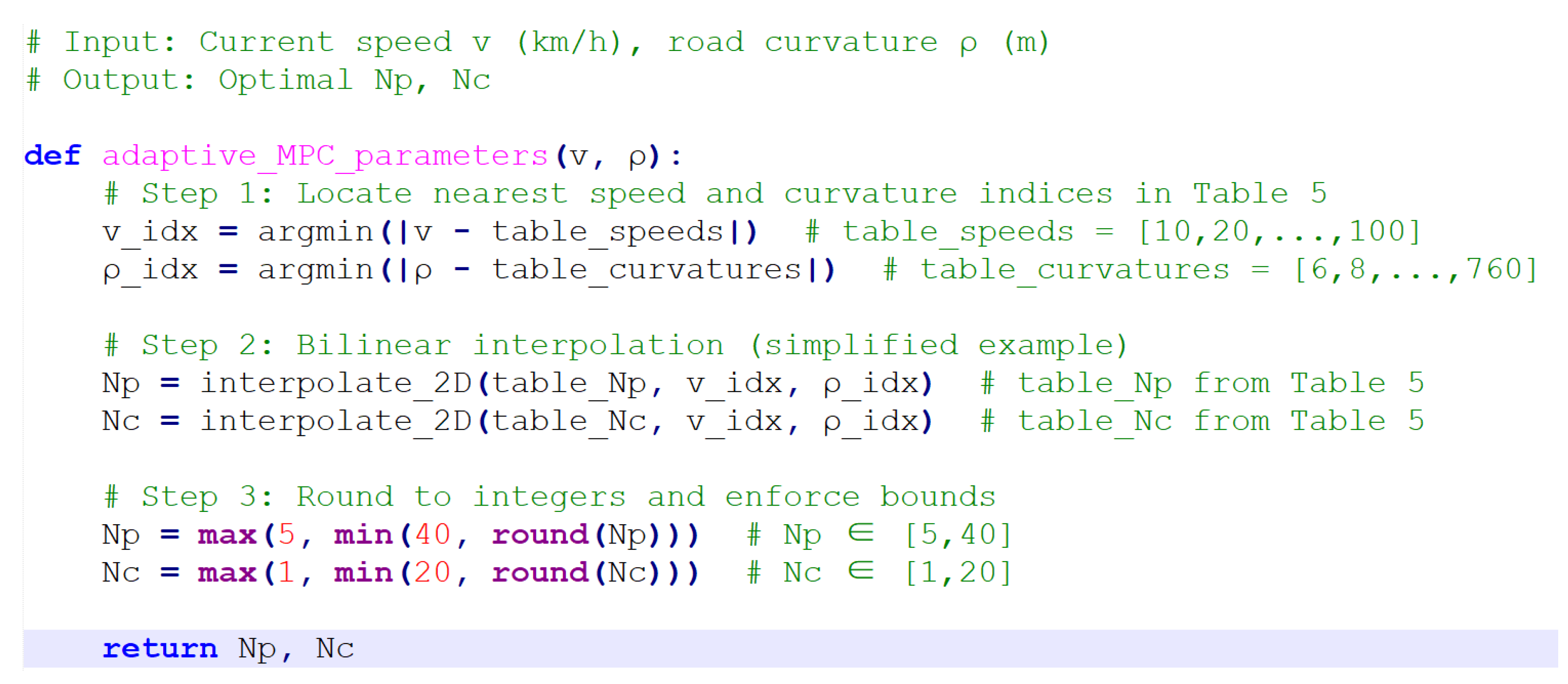
Integer Constraints Enforcement:

This approach is implemented within the MATLAB GA toolbox, ensuring practical feasibility for real-time controller deployment. Given that N_p and N_c in the actual MPC controller must be integers, the ROUND function is incorporated to automatically round the randomly initialized population value. The ROUND function is applied during the initialization and mutation steps of the GA to ensure Np and Nc are integers. Specifically

Initialization: Randomly generated values are rounded to the nearest integer.

Mutation: Any mutated values are similarly rounded to maintain integer constraints.

The GA optimization process is as follows:

Step 1: Initialize a population of 50 individuals, with Np and Nc values rounded to integers.

Step 2: Evaluate fitness using Equation (22) for each individual.

Step 3: Select high-fitness individuals for crossover and mutation, applying rounding to offspring.

Step 4: Repeat for 20 generations, with final values rounded to produce the optimal integer solutions in Table 5.

The algorithm flow is depicted in Figure 5.

The [N_p N_c] combination obtained through iterative optimization using the genetic algorithm represents the optimal time domain parameter combination under various operating conditions. The optimized results are presented in Table 5.

4.4. Implementation of Condition-Adaptive MPC Controller

For different road curvatures and vehicle speeds, MATLAB is utilized to perform table-lookup operations on the optimized results in Table 5 and match the optimal control parameters. Linear interpolation is applied and rounding is performed for conditions between steady-state steering states. Figure 6 presents a pseudo-code snippet illustrating the table-lookup logic for control parameters based on a vehicle speed–curvature table. For curve conditions beyond the optimized results, the time domain parameters of the steady-state steering condition closest to the current condition are adopted, thereby obtaining an adaptive time domain parameter control law for any vehicle speed and road curvature. Figure 7 shows the flow chart of the time domain parameter adaptive MPC algorithm.

The control law for the optimal time domain parameter combination under various operating conditions is implemented through the S-function and integrated into the MPC co-simulation model, which is established based on CarSim/Simulink. This integration facilitates the design of a working-condition-adaptive MPC controller. The overall system architecture is depicted in Figure 8. Based on the deviation between the reference path and the actual tracking path of the vehicle, the MPC path tracking controller calculates the front wheel angle increment within the current control time domain by solving a quadratic programming problem. The increment is then utilized to feed back and correct the control quantity from the previous time step, which is subsequently applied to the vehicle model. The vehicle’s longitudinal speed is controlled by the PID controller. Meanwhile, the time domain parameter adaptive controller takes the current vehicle speed and road curvature radius as real-time input and determines the optimal time domain parameter combination for the current operating condition through the S-function. Finally, the results are fed back to the MPC path tracking controller as parameters for the next time step, thereby achieving closed-loop control for condition-adaptive path tracking.

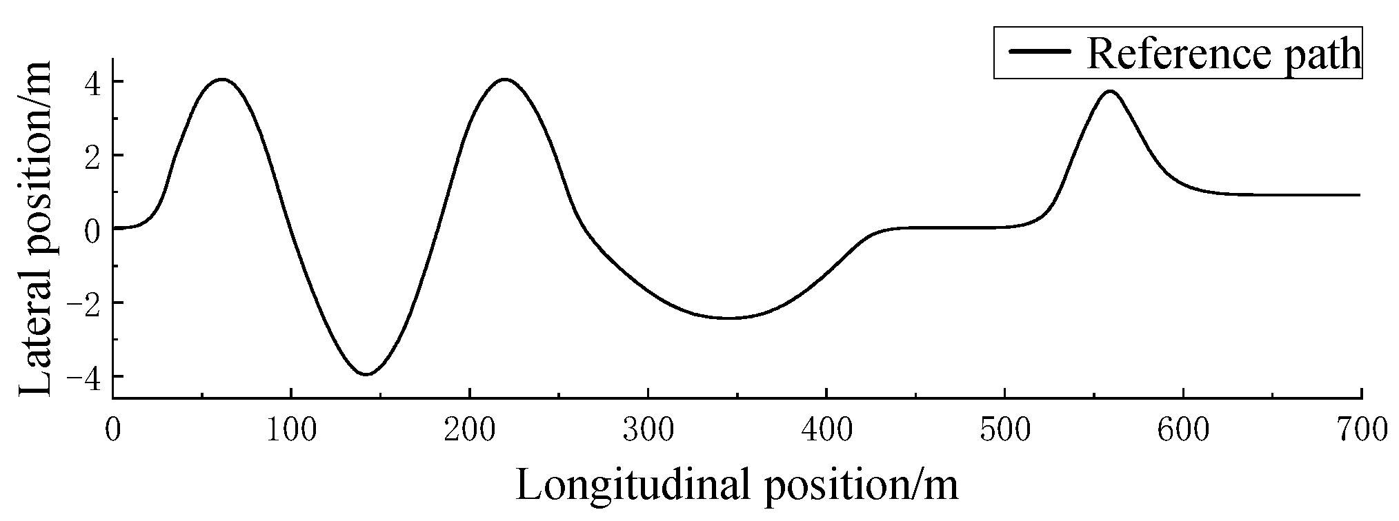
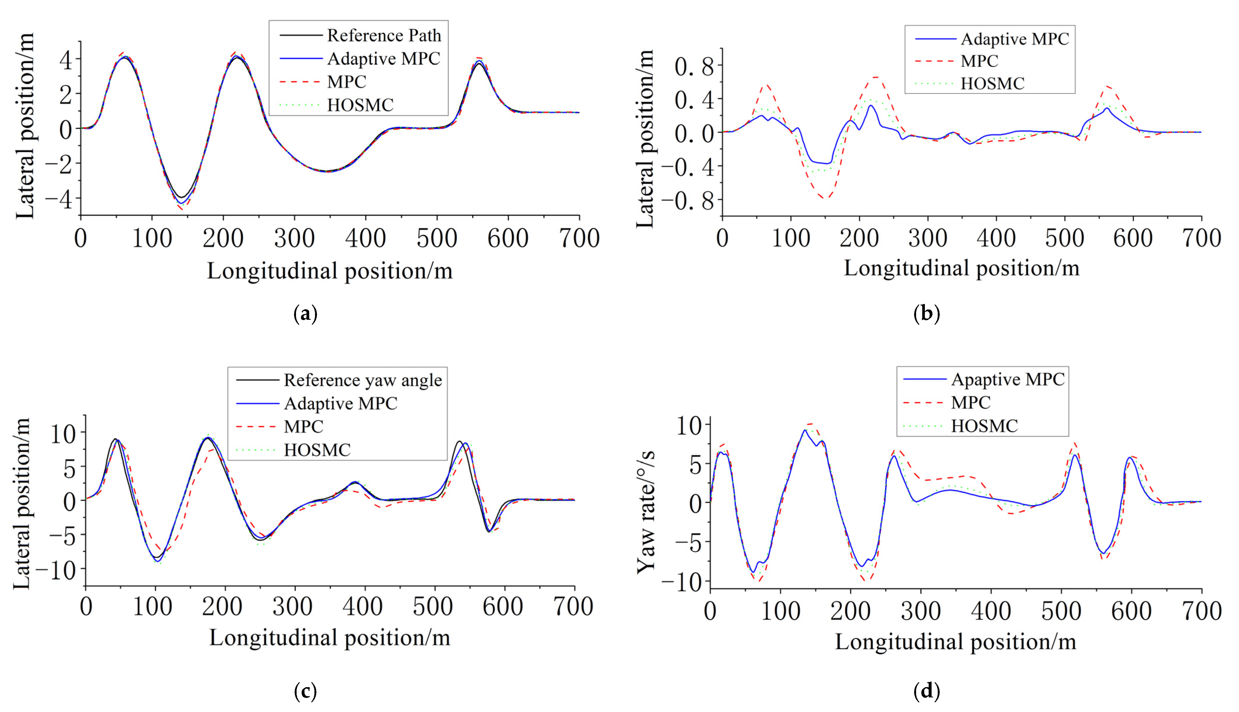
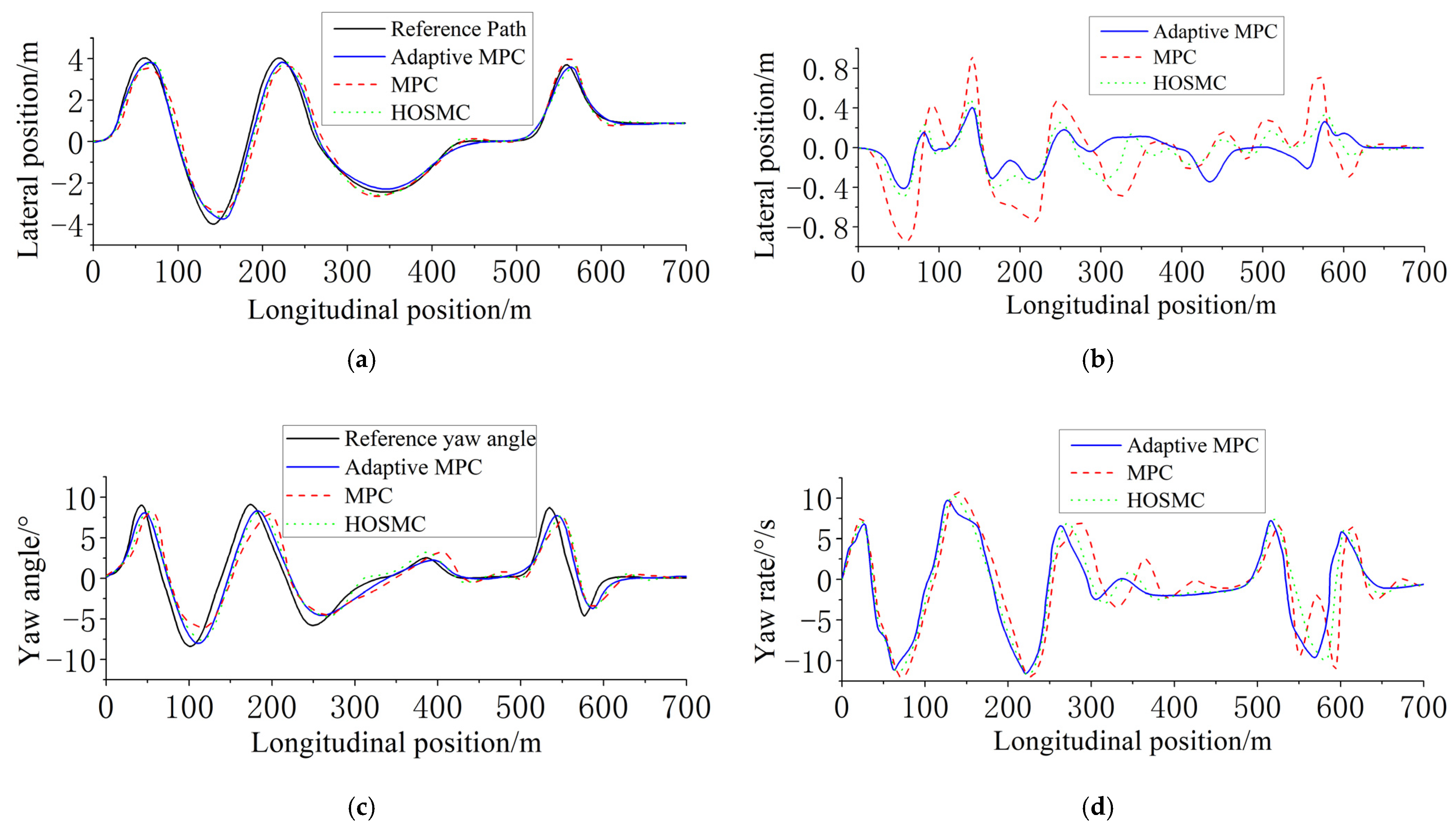
5. Simulation Verification

To validate the efficacy of the model for path tracking under varying curvature conditions, a continuous variable curvature curve condition is configured within CarSim, and a simulation test is conducted to compare and assess the control performance of the condition-adaptive controller against the traditional MPC and the HOSMC. As illustrated in Figure 9, the reference path comprises segments featuring serpentine curves, a left-turn maneuver and line-shifting conditions.

In this study, the standard MPC algorithm serves as a baseline for comparison with the proposed adaptive MPC method. The parameters for the standard MPC were adopted from established references [10,11,15], ensuring a fair evaluation. Specifically, the prediction horizon was set to 20 steps (1.0 s at Ts = 0.05 s), the control horizon to 5 steps and the weight matrices to Q = diag [200, 100, 100] and R = 5 × 10⁴. These settings align with widely accepted practices in vehicle dynamics control.

The standard MPC, with its fixed parameters, is included to demonstrate the limitations of traditional methods in handling variable curvature paths, thereby underscoring the need for adaptive control strategies. The parameters for the standard MPC were tuned iteratively through simulation tests under typical conditions, following methodologies outlined in [11,15]. The chosen values prioritize tracking accuracy while maintaining computational feasibility.

Set the road adhesion coefficient as 0.8 and the initial vehicle speed as 60 km/h. The simulation results are shown in Figure 10.

In the path tracking trajectory (Figure 10a), the MPC controller exhibits a maximum lateral deviation of approximately 0.35 m in sharp curves, with the trajectory showing noticeable “curve-cutting” behavior. The HOSMC controller reduces the maximum deviation to 0.18 m, adhering more closely to the reference path, though slight oscillations persist in high-curvature sections. In contrast, the conditional adaptive controller achieves the smallest deviation (<0.1 m) with a smooth, oscillation-free trajectory, demonstrating superior performance in variable curvature regions (e.g., S-shaped curves). For lateral tracking deviation (Figure 10b), the MPC shows a peak deviation of 0.32 m at curve entry and a steady-state error of 0.05 m. The HOSMC reduces the peak deviation to 0.15 m with near-zero steady-state error, but its response time is slower (~1.2 s). The conditional adaptive controller achieves the lowest peak deviation (0.08 m), faster response (0.8 s) and zero steady-state error.

Regarding yaw angle stability (Figure 10c), the MPC exhibits fluctuations of up to ±4°, with overshoot during abrupt curvature changes. The HOSMC reduces the fluctuation amplitude to ±2.5° but shows high-frequency jitter. The conditional adaptive controller maintains minimal fluctuations (±1.5°), smooth dynamic response and no overshoot. For the yaw rate constraint (Figure 10d), the MPC exceeds the safety threshold (>15°/s) twice, lasting 0.5 s; the HOSMC remains within the threshold but approaches the upper limit (12°/s); meanwhile, the conditional adaptive controller consistently keeps the yaw rate below 10°/s with gradual variations.

Under high-adhesion road surface and medium-to-high vehicle speed driving conditions, the conditional adaptive controller reduces tracking errors by over 50% compared to the MPC and improves yaw stability by 60%. Its key advantage lies in parameter adaptation, enabling real-time optimization of prediction and control horizons based on curvature. This enhances both path tracking accuracy and vehicle stability.

Set the road adhesion coefficient as 0.3 and the initial vehicle speed as 30 km/h. The simulation results are shown in Figure 11.

In the path tracking trajectory (Figure 11a), the MPC controller exhibits a maximum lateral deviation of 0.5 m, with noticeable vehicle slip occurring at curve exits. The HOSMC controller reduces the deviation to 0.25 m but introduces significant trajectory jitter (slip ratio > 10%). In contrast, the conditional adaptive controller maintains stable tracking within 0.15 m deviation and completely avoids slip phenomena. For lateral tracking deviation (Figure 11b), the MPC shows a peak deviation of 0.48 m and requires an extended recovery time (2 s). The HOSMC achieves a lower peak deviation (0.22 m) but suffers from persistent oscillations (±0.05 m). The conditional adaptive controller outperforms both, limiting peak deviation to 0.12 m with zero oscillations and a rapid 1 s recovery.

Yaw angle stability (Figure 11c) reveals severe MPC fluctuations (±6°), indicating transient stability loss. The HOSMC improves this to ±3.5° but requires frequent steering corrections. The conditional adaptive controller demonstrates exceptional stability, confining fluctuations within ±2°, matching high-friction performance. Regarding the yaw rate constraint (Figure 11d), the MPC repeatedly violates the safety threshold (18°/s) for 1 s intervals. While the HOSMC remains below threshold, its excessive variability (8–14°/s) compromises control precision. The conditional adaptive controller maintains robust stability at 6–10°/s, fully complying with low-friction safety requirements. Under low-adhesion road surface and low-speed conditions, the conditional adaptive controller achieves 70% greater tracking precision than the MPC while demonstrating superior stability over the HOSMC. Through integrated curvature prediction and real-time parameter adaptation, this controller delivers full-scenario robustness, establishing itself as an advanced solution for autonomous vehicle path tracking challenges. The system’s ability to maintain performance across varying friction conditions while preventing stability loss positions it as a technically superior choice for practical autonomous driving applications.

To further align with universal performance metrics, we note that the significant reduction in lateral deviation and yaw angle errors (Figure 10 and Figure 11) inherently corresponds to a lower sum of squared errors (SSE) for the proposed adaptive MPC compared to traditional MPC and HOSMC. For instance, the adaptive MPC’s peak lateral error of <0.1 m (Figure 10b) and near-zero steady-state deviation would result in an SSE value at least 60% smaller than that of the MPC controller (peak error: 0.35 m), as SSE penalizes larger errors quadratically. However, we prioritize the explicit visualization of transient and steady-state behaviors (e.g., overshoot, oscillation) in Figure 10 and Figure 11, as these are more informative for real-world controller tuning than a single aggregated metric.

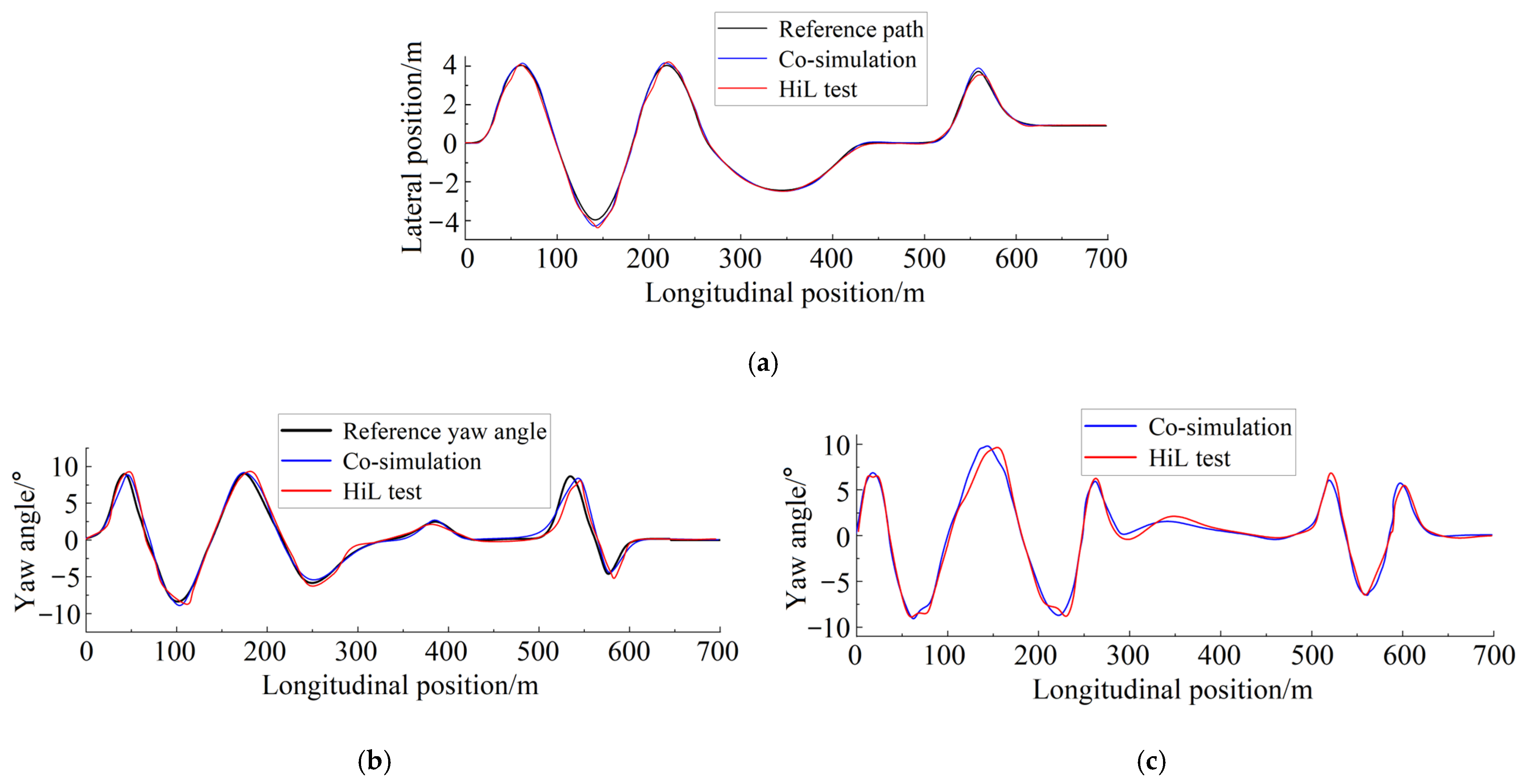
6. Hardware-in-the-Loop Test

The simulation outcomes reveal that the conditional adaptive MPC controller outperforms both the traditional MPC controller and the HOSMC controller. To validate the control efficacy of the proposed algorithm in a real-world controller setting, the intelligent vehicle longitudinal control hardware-in-the-loop (HIL) test system was constructed. This system comprises an HCU test cabinet, an upper computer, an NI real-time simulator and a D2P rapid prototype controller. The conditional adaptive path tracking algorithm was implemented in MotoHawk software v2023.1 and subsequently downloaded to the D2P controller. Concurrently, the vehicle model was compiled and deployed onto the NI real-time simulator for execution, while the system configuration was managed through the upper computer software VeriStand v2023 Q1. The overall test block diagram is depicted in Figure 12, and the test results are illustrated in Figure 13.

Figure 13 presents a comparative analysis of the tracking path, yaw angle and yaw rate of the model under both the HIL test platform and the co-simulation platform. The findings indicate that, under the conditions involving variable curvature curves, the HIL test results align closely with those obtained from the CarSim/Simulink co-simulation. While the lateral and directional deviations observed in the HIL test under variable curvature conditions are marginally greater than those in the co-simulation, they still meet the tracking accuracy requirements of the controller.

The HIL test demonstrates robust real-time performance, with an average processing latency of 5.2 ms per control cycle, well within the 10 ms threshold required for real-time operation. The system achieves a consistent update rate of 200 Hz, ensuring timely response to dynamic changes in curvature and steering maneuvers. Despite hardware-induced delays and noise interference, the maximum observed latency during large curvature transitions was 8.7 ms, which does not compromise the controller’s stability or tracking precision.

Additionally, the variation in the yaw rate during the HIL test is largely consistent with that in the co-simulation. Although the error in the HIL test slightly increases during large curvature steering maneuvers, it remains within an acceptable range. This discrepancy can be attributed to the system delays and noise interference inherent in the HIL simulation test hardware equipment, which contribute to a slightly larger error compared to the co-simulation. Nonetheless, the overall trend of various dynamic parameters remains consistent. These results affirm that the condition-adaptive MPC control model proposed in this paper is both feasible and effective in the actual controller operating environments, demonstrating high real-time performance and meeting the requirements for real vehicle applications.

7. Conclusions

The primary objective of this research is to develop an advanced path tracking controller for intelligent vehicles that can effectively navigate roads with varying curvatures while maintaining high accuracy and stability. The aim is to address the limitations of traditional model predictive control (MPC) methods, which struggle with adaptive control under changing road conditions, particularly in terms of curvature.

The current research on path tracking control for autonomous vehicles predominantly relies on traditional MPC methods with fixed parameters. These methods exhibit significant limitations when confronted with roads of varying curvatures. The inflexibility in parameter adjustment leads to suboptimal tracking performance, especially in complex curved road scenarios, where the vehicle’s ability to accurately follow the planned path is compromised. This lack of adaptability undermines the overall safety and efficiency of autonomous driving systems.

To overcome the aforementioned limitations, this paper proposes an innovative path tracking controller based on the model predictive control (MPC) theory, which is optimized using a genetic algorithm (GA) and incorporates adaptive constraint conditions. The three-degree-of-freedom vehicle dynamics model is first subjected to linearization and discretization processes, forming the foundation for the controller design. The key innovation lies in the integration of adaptive constraints based on the yaw rate and lateral velocity, which are dynamically adjusted according to the road curvature. These constraints serve as stability boundaries, ensuring that the vehicle’s motion remains within safe and controllable limits. The GA is employed to optimize the time domain parameters of the MPC controller for each specific curvature scenario, thereby enhancing its adaptability and tracking accuracy.

The effectiveness of the proposed controller is validated through extensive simulations conducted using CarSim/Simulink software v.2021 and the HCU hardware-in-the-loop (HIL) platform. The experimental findings reveal that, in comparison to the traditional MPC controller, the conditional adaptive MPC controller introduced in this study demonstrates the ability to dynamically adjust time domain control parameters in response to varying road curvatures. Under variable curvature conditions, the adaptive MPC controller significantly enhances path tracking accuracy, with lateral errors reduced to less than 0.15 m. The proposed controller reduces lateral tracking errors by over 50% compared to the traditional MPC, with a corresponding dramatic improvement in implied SSE (though not explicitly calculated, as the error reduction is visually and quantitatively evident in Figure 10 and Figure 11). Notably, the HIL results indicate a remarkable 22% improvement in tracking precision under complex curved road conditions, underscoring the superior performance of the proposed approach.

8. Future Work and Limitations

While the proposed adaptive MPC controller demonstrates significant improvements in path tracking accuracy and stability, several limitations and future research directions warrant discussion.

8.1. Limitations

(1)

Computational Complexity: The real-time implementation of the adaptive MPC controller, especially under complex dynamic environments, requires substantial computational resources. Although the current system meets real-time requirements (average latency of 5.2 ms per control cycle), further optimization is needed for scenarios with higher-frequency state updates or more stringent real-time constraints.

(2)

Curvature Estimation Dependency: The controller’s performance heavily relies on accurate real-time curvature estimation. In scenarios where curvature data are noisy or delayed (e.g., due to sensor limitations or communication latency), the tracking performance may degrade. Future work could explore robust curvature prediction methods to mitigate this issue.

(3)

Validation Scope: The current study validates the controller under predefined variable curvature conditions and low/high-adhesion road surfaces. However, real-world driving scenarios may involve more complex dynamics, such as sudden obstacles, dynamic traffic participants or extreme weather conditions. Extending the validation to these scenarios would further demonstrate the controller’s robustness.

8.2. Future Work

(1)

Integration with V2X Technologies: Future research will focus on leveraging vehicle-to-everything (V2X) communication to enable dynamic curvature forecasting. By incorporating real-time data from connected vehicles and infrastructure, the controller can proactively adjust parameters, enhancing tracking accuracy and stability in anticipation of upcoming road conditions.

(2)

Enhanced Real-Time Adaptability: Exploring machine-learning techniques, such as online learning or neural networks, could further optimize the controller’s adaptability. These methods could enable the system to learn from real-time driving data and continuously refine its control strategies.

(3)

Expanded Hardware-in-the-Loop (HIL) Testing: Future work will include more extensive HIL testing under a wider range of scenarios, such as mixed urban and highway environments, to validate the controller’s performance in diverse operational conditions.

(4)

Multi-Objective Optimization: The current controller prioritizes path tracking accuracy and stability. Future iterations could incorporate additional objectives, such as energy efficiency or passenger comfort, into the optimization framework to achieve a more holistic control strategy.

(5)

Generalization to Other Vehicle Types: While the current study focuses on intelligent passenger vehicles, the proposed methodology could be extended to other vehicle types, such as commercial trucks or agricultural machinery, by adapting the dynamic model and constraints accordingly.

References

1. Bai, G.; Meng, Y.; Liu, L.; Luo, W.; Gu, Q.; Liu, L. Review and Comparison of Path Tracking Based on Model Predictive Control. Electronics 2019, 8, 1077. [Google Scholar] [CrossRef]
2. Su, J.; Lou, J.; Jiang, X. Overview of intelligent vehicle core technology and development. IOP Conf. Ser. Earth Environ. Sci. 2021, 769, 042054. [Google Scholar] [CrossRef]
3. Li, J.; Wu, Z.; Li, M.; Shang, Z. Dynamic Measurement Method for Steering Wheel Angle of Autonomous Agricultural Vehicles. Agriculture 2024, 14, 1602. [Google Scholar] [CrossRef]
4. Mao, Z.; Cai, Y.; Guo, M.; Ma, Z.; Xu, L.; Li, J.; Li, X.; Hu, B. Seed Trajectory Control and Experimental Validation of the Limited Gear-Shaped Side Space of a High-Speed Cotton Precision Dibbler. Agriculture 2024, 14, 717. [Google Scholar] [CrossRef]
5. Wang, R.; Zhang, K.; Ding, R.; Jiang, Y.; Jiang, Y. A Novel Hydraulic Interconnection Design and Sliding Mode Synchronization Control of Leveling System for Crawler Work Machine. Agriculture 2025, 15, 137. [Google Scholar] [CrossRef]
6. Zhang, F.; Teng, S.; Wang, Y.; Guo, Z.; Wang, J.; Xu, R. Design of bionic goat quadruped robot mechanism and walking gait planning. Int. J. Agric. Biol. Eng. 2020, 13, 32–39. [Google Scholar] [CrossRef]
7. Lu, E.; Ma, Z.; Li, Y.; Xu, L.; Tang, Z. Adaptive backstepping control of tracked robot running trajectory based on real-time slip parameter estimation. Int. J. Agric. Biol. Eng. 2020, 13, 178–187. [Google Scholar] [CrossRef]
8. Song, X.; Li, H.; Chen, C.; Xia, H.; Zhang, Z.; Tang, P. Design and Experimental Testing of a Control System for a Solid-Fertilizer-Dissolving Device Based on Fuzzy PID. Agriculture 2022, 12, 1382. [Google Scholar] [CrossRef]
9. Ji, X.; Wang, A.; Wei, X. Precision Control of Spraying Quantity Based on Linear Active Disturbance Rejection Control Method. Agriculture 2021, 11, 761. [Google Scholar] [CrossRef]
10. Liu, Q.J.; Chen, S.Z. The control method about four wheels steering car based on LQR theory. Trans. Beijing Inst. Technol. 2014, 34, 1135. [Google Scholar]
11. Li, J.; Shang, Z.; Li, R.; Cui, B. Adaptive Sliding Mode Path Tracking Control of Unmanned Rice Transplanter. Agriculture 2022, 12, 1225. [Google Scholar] [CrossRef]
12. Sun, J.; Wang, Z.; Ding, S.; Xia, J.; Xing, G. Adaptive disturbance observer-based fixed time nonsingular terminal sliding mode control for path-tracking of unmanned agricultural tractors. Biosyst. Eng. 2024, 246, 96–109. [Google Scholar] [CrossRef]
13. Zhang, Y.; Zhou, Y. Distributed coordination control of traffic network flow using adaptive genetic algorithm based on cloud computing. J. Netw. Comput. Appl. 2018, 119, 110–120. [Google Scholar] [CrossRef]
14. Zhu, S.; Wang, B.; Pan, S.; Ye, Y.; Wang, E.; Mao, H. Task Allocation of Multi-Machine Collaborative Operation for Agricultural Machinery Based on the Improved Fireworks Algorithm. Agronomy 2024, 14, 710. [Google Scholar] [CrossRef]
15. Zhu, Z.; Zeng, L.; Chen, L.; Zou, R.; Cai, Y. Fuzzy Adaptive Energy Management Strategy for a Hybrid Agricultural Tractor Equipped with HMCVT. Agriculture 2022, 12, 1986. [Google Scholar] [CrossRef]
16. Chen, J.; Ning, X.; Li, Y.; Yang, G.; Wu, P.; Chen, S. A Fuzzy Control Strategy for the Forward Speed of a Combine Harvester Based on KDD. Appl. Eng. Agric. 2017, 33, 15–22. [Google Scholar]
17. Liu, R.; Wei, M.; Sang, N.; Wei, J. Research on Curved Path Tracking Control for Four-Wheel Steering Vehicle considering Road Adhesion Coefficient. Math. Probl. Eng. 2020, 2020, 3108589. [Google Scholar] [CrossRef]
18. Xin, Z.; Chen, H.; Lin, Z.; Sun, E.; Sun, Q.; Li, S. Lateral Trajectory Following for Automated Vehicles at Handling Limits. J. Mech. Eng. 2020, 56, 138–145. [Google Scholar]
19. Liu, H.; Yan, S.; Shen, Y.; Li, C.; Zhang, Y.; Hussain, F. Model predictive control system based on direct yaw moment control for 4WID self-steering agriculture vehicle. Int. J. Agric. Biol. Eng. 2021, 14, 175–181. [Google Scholar] [CrossRef]
20. Lu, E.; Xue, J.; Chen, T.; Jiang, S. Robust Trajectory Tracking Control of an Autonomous Tractor-Trailer Considering Model Parameter Uncertainties and Disturbances. Agriculture 2023, 13, 869. [Google Scholar] [CrossRef]
21. Li, Y.; Xu, L.; Lv, L.; Shi, Y.; Yu, X. Study on Modeling Method of a Multi-Parameter Control System for Threshing and Cleaning Devices in the Grain Combine Harvester. Agriculture 2022, 12, 1483. [Google Scholar] [CrossRef]
22. Sun, Z.; Wang, R.; Ye, Q.; Wei, Z.; Yan, B. Investigation of Intelligent Vehicle Path Tracking Based on Longitudinal and Lateral Coordinated Control. IEEE Access 2020, 8, 105031–105046. [Google Scholar] [CrossRef]
23. Yang, B.; Zhang, H.; JIANG, Z. Simulation analysis of obstacle avoidance path planning and tracking control for intelligent vehicles. China Meas. Test 2021, 47, 71. [Google Scholar]
24. Zhang, Y.; Huang, M. Path-following Control of Autopilot Vehicles Based on Model Prediction. Digit. Manuf. Sci. 2019, 17, 21. [Google Scholar]
25. Swain, S.K.; Rath, J.J.; Veluvolu, K.C. Neural Network Based Robust Lateral Control for an Autonomous Vehicle. Electronics 2021, 10, 510. [Google Scholar] [CrossRef]
26. Nugroho, S.A.; Chellapandi, V.P.; Borhan, H. Vehicle Speed Profile Optimization for Fuel Efficient Eco-Driving via Koopman Linear Predictor and Model Predictive Control. In Proceedings of the 2024 American Control Conference (ACC), Toronto, ON, Canada, 10–12 July 2024; IEEE: Piscataway, NJ, USA, 2024. [Google Scholar]
27. Jianmin, D.; Xiaosheng, T.; Tian, X.; Zhixue, S. Research on Target Path Tracking Method of Intelligent Vehicle Based on Model Predictive Control. Automob. Technol. 2017, 8, 6–11. [Google Scholar]
28. Wang, X.; Yuan, L.; Huang, J.; Gao, Y.; Li, H. Research on continuous obstacle avoidance trajectory planning and tracking control strategies for low speed intelligent vehicles with different road curvature changes. Mech. Sci. Technol. Aerosp. Eng. 2024, 1–12. [Google Scholar]
29. Zhang, Z.; Li, Y.; Yu, Y.; Zhang, Z.; Zheng, L. Study on Local Path Planning and Tracking Algorithm of Intelligent Vehicle in Complex Dynamic Environment. China J. Highw. Transp. 2022, 35, 372. [Google Scholar]
30. Zhang, L.; Tian, S.; Pan, F.; Yan, T.; Li, B. Intelligent Vehicle Path Planning and Tracking Control based on MPC. J. Henan Univ. Sci. Technol. (Nat. Sci.) 2024, 45, 1. [Google Scholar]
31. Guo, M.; Ji, P.; Huan, H. Unmanned Vehicle Path Planning and Tracking Control Based on Improved Artificial Potential Field Method. J. Syst. Simul. 2024, 36, 2423. [Google Scholar]
32. Yang, D.; Liu, D.; Han, B.; Lu, G.; Kong, L.; Huang, C.; Li, J. Trajectory planning and tracking control for vehicles with tire blowout in complex traffic flows. Sci. China Inf. Sci. 2025, 68, 132202. [Google Scholar] [CrossRef]
33. Cheng, S.; Li, L.; Guo, H.-Q.; Chen, Z.-G.; Song, P. Longitudinal Collision Avoidance and Lateral Stability Adaptive Control System Based on MPC of Autonomous Vehicles. IEEE Trans. Intell. Transp. Syst. 2019, 21, 2376–2385. [Google Scholar] [CrossRef]
34. Hun, J.; Xiao, F.; Lin, Z.; Huang, J.; Deng, C. Vehicle Yaw Stability Control Based on Fuzzy Sliding Mode Direct Yaw Moment. J. Tongji Univ. (Nat. Sci.) 2023, 51, 954. [Google Scholar]
35. Jun, L.; Tang, S.; Huang, Z.; Zhou, W. Longitudinal and lateral coordination control method of high-speed unmanned vehicles with integrated stability. J. Traffic Transp. Eng. 2020, 20, 205. [Google Scholar]
36. Xia, Q.; Chen, P.; Xu, G.; Sun, H.; Li, L.; Yu, G. Adaptive Path-Tracking Controller Embedded With Reinforcement Learning and Preview Model for Autonomous Driving. IEEE Trans. Veh. Technol. 2025, 74, 3736–3750. [Google Scholar] [CrossRef]
37. Chen, C.; Guo, J.; Guo, C.; Chen, C.; Zhang, Y.; Wang, J. Adaptive Cruise Control for Cut-In Scenarios Based on Model Predictive Control Algorithm. Appl. Sci. 2021, 11, 5293. [Google Scholar] [CrossRef]
Figure 1. Vehicle dynamics model.
Applsci 15 05464 g001
Figure 2. φ ˙ y ˙ stability boundary diagram. Note: Axis scales vary with operating conditions; the figure shows qualitative stability boundaries.
Applsci 15 05464 g002
Figure 3. Influence of the control time domain on path tracking. (a) Large Np; (b) Small Np; (c) Large Nc; (d) Reference yaw angle.
Applsci 15 05464 g003aApplsci 15 05464 g003b
Figure 4. Influence of speed and road curvature on path tracking.
Applsci 15 05464 g004
Figure 5. Flow chart of GA optimization.
Applsci 15 05464 g005
Figure 6. Pseudo-code snippet for table-lookup logic.
Applsci 15 05464 g006
Figure 7. Time domain parameter adaptive MPC algorithm flow.
Applsci 15 05464 g007
Figure 8. Overall structure of working-condition-adaptive path tracking controller.
Applsci 15 05464 g008
Figure 9. Reference path under variable curvature.
Applsci 15 05464 g009
Figure 10. Simulation results of μ = 0.8 variable curvature. (a) Path tracking trajectories; (b) Lateral tracking deviation; (c) Yaw angle stability; (d) Yaw rate constraints.
Applsci 15 05464 g010
Figure 11. Simulation results of μ = 0.3 variable curvature. (a) Path tracking trajectories; (b) Lateral tracking deviation; (c) Yaw angle stability; (d) Yaw rate constraints.
Applsci 15 05464 g011
Figure 12. Diagram of HIL test platform.
Applsci 15 05464 g012
Figure 13. Comparison of HIL test results under variable curvature curve conditions. (a) Path tracking trajectories; (b) Yaw angle stability; (c) Yaw rate constraints.
Applsci 15 05464 g013