

Classification of Multiple Partial Discharge Sources Using Time-Frequency Analysis and Deep Learning


Abstract
1. Introduction
1.1. Challenges in Multiple PD Source Classification
1.2. Literature Review
1.3. Effective Proposed Approaches for Classifying Multiple PD Sources
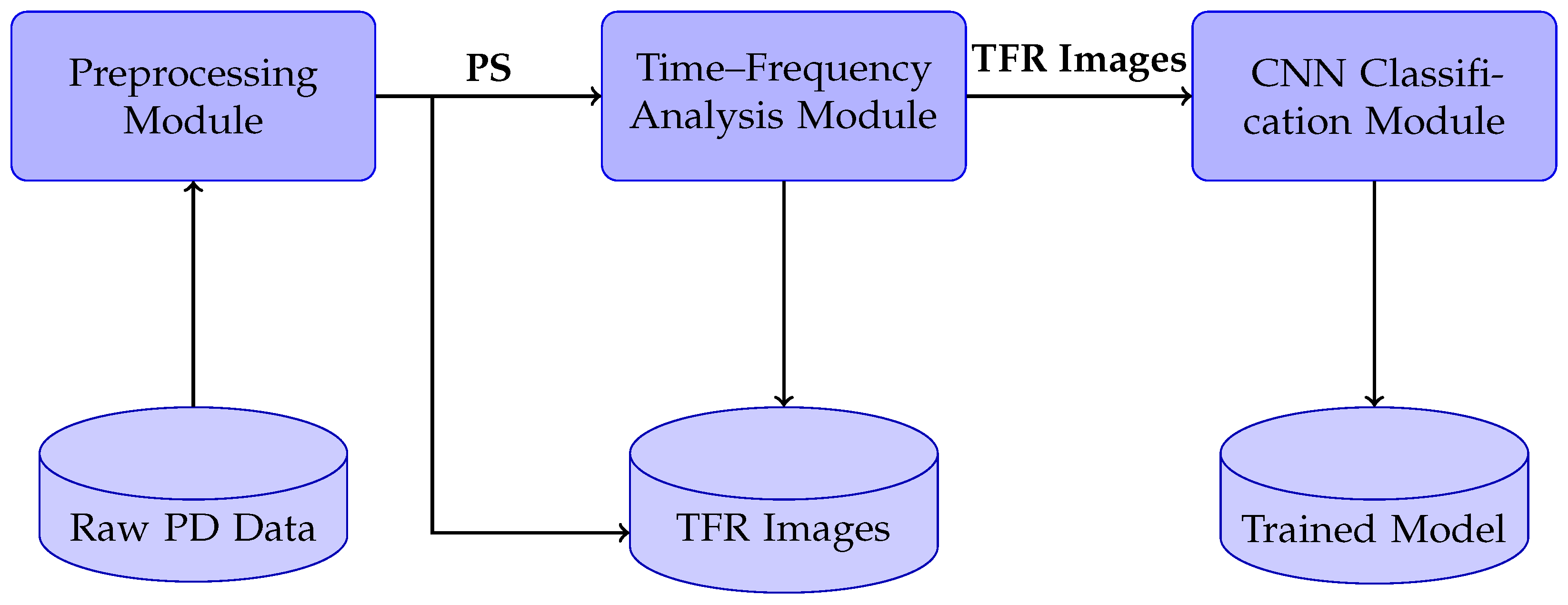
1.3.1. Database

1.3.2. Time–Frequency Features
1.3.3. Deep Learning
1.4. Motivation for the Proposed Approach
2. FEM in Partial Discharge Simulation
2.1. Simulation Framework
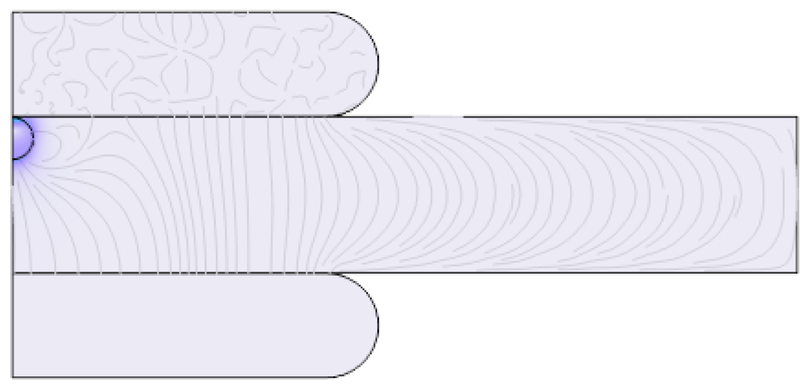
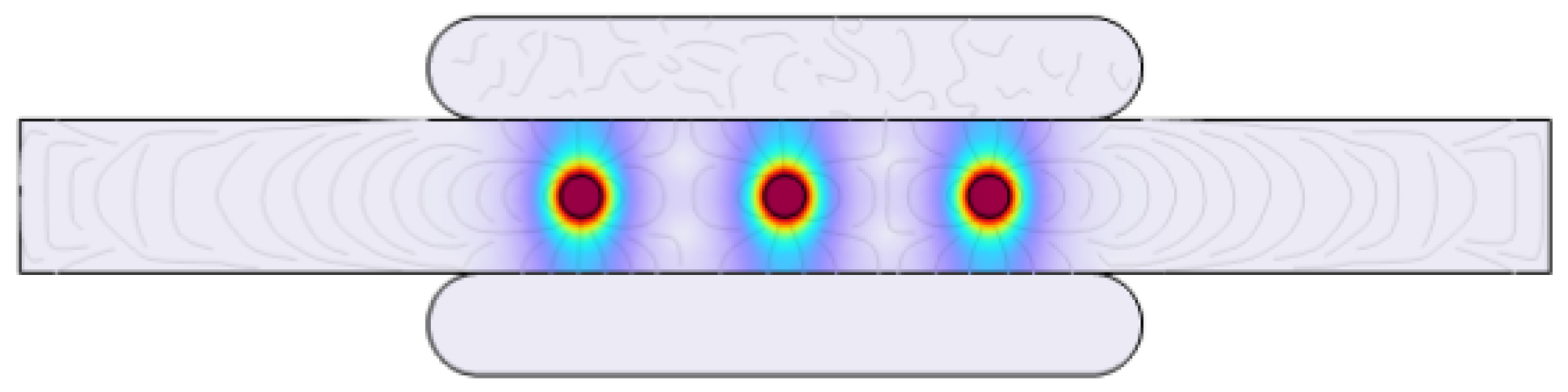
2.1.1. Geometry and Model Setup
2.1.2. Material Characteristics
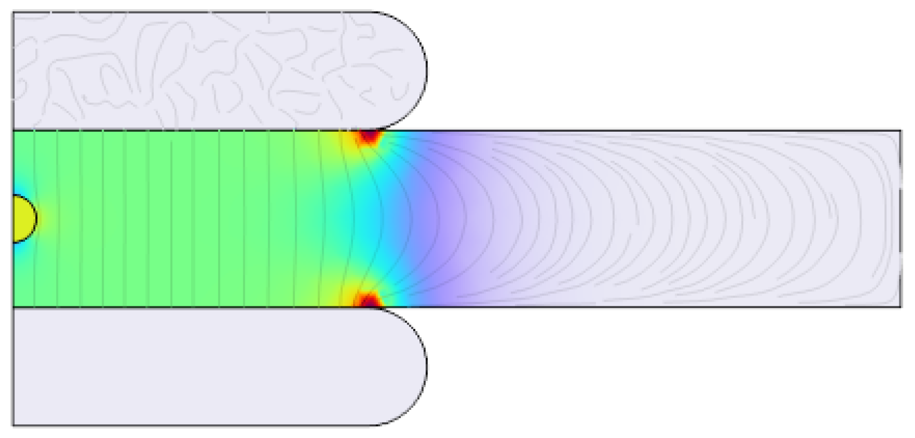
2.1.3. Application of Physics Interfaces
- I.
- Electrostatic and Space Charge Modeling
- (a)
- Poisson’s Equation
- (b)
- Charge Transport Equations
- II.
- Stochastic Modeling

- (a)
- Exponential Model
- (b)
- CDF for PD Event
- (c)
- Random Number Comparison
2.1.4. Electrical Boundary Conditions
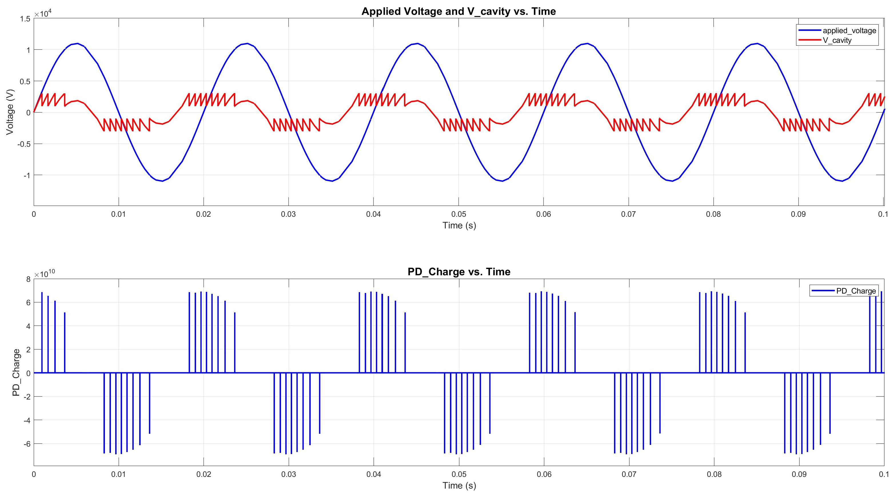
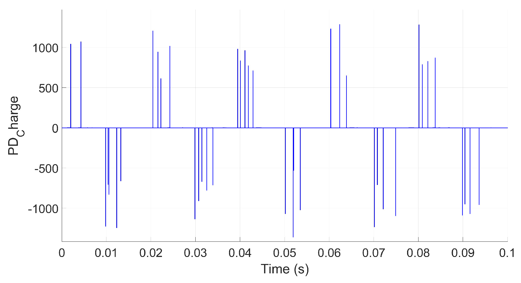
2.1.5. PD Simulation Parameters
2.1.6. Mesh and Solver Settings
- Mesh: A finer mesh was applied near the cavity and electrode boundaries for accurate field resolution.
- Solver: Transient study with adaptive time stepping to resolve rapid changes during PD events.


2.2. Simulation Scenarios
2.2.1. Simulation Scenario I: Single Cavity with Varying Positions


2.2.2. Simulation Scenario II: Impact of Varying Cavity Shapes, Alignments, and Stacking


2.2.3. Simulation Scenario III: Impact of Size, Shape, and Multiple PD Sources on Rate of Occurrence


3. Experimental Measurements
- : wavelet basis functions (sym4);
- : detail coefficients;
- : approximation coefficients;
- : decomposition level.


- Fixed-Window Segmentation: Partition the signal into consistent, equally-sized segments.
- Event-Based Segmentation: Subdivide the signal according to identified PD events. The energy-based detection identifies pulses using:
| Algorithm 1 PD Signal Preprocessing |
|

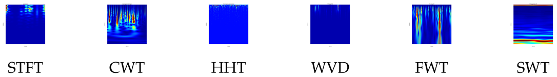
4. Time–Frequency Analysis for Feature Extraction
4.1. Short-Time Fourier Transform (STFT)
4.2. Wavelet Transform (WT)
4.3. Wigner–Ville Distribution (WVD)
4.4. Hilbert–Huang Transform (HHT)
4.4.1. Empirical Mode Decomposition (EMD)
4.4.2. Hilbert Spectral Analysis (HSA)
4.5. Fractional Wavelet Transform (FRWT)
4.6. Wavelet Scattering Transform (WST)
5. Classification of PD Sources via DL Model
6. Results and Discussion
6.1. Comparative Performance Analysis
- The superiority of the Scatter Wavelet Transform (SWT):achieved perfect classification with ResNet50, confirming its robustness in handling real-world noise and multi-source PD patterns.
- The consistency of the Wigner–Ville Distribution (WVD):demonstrated stable performance, though its quadratic computation introduces trade-offs between resolution and cross-term artifacts.
6.2. Method-Specific Insights
6.2.1. High-Performance Methods
- The SWT’s Advantage: The scattering network’s invariance to small deformations explains its experimental dominance:
- The WVD’s Trade-off: While achieving 94.74% experimental accuracy, its performance is bounded by the Heisenberg uncertainty principle:
6.2.2. Suboptimal Performance of Methods
- Sensitivity of the Hilbert-Huang Transform (HHT): The experiments exhibited a substantial reduction in accuracy by 18.33%, attributed to:
- –
- The instability of Empirical Mode Decomposition (EMD) when subjected to experimental noise, which undermines its robustness;
- –
- The presence of end effects, which significantly skew the evaluation of instantaneous frequency.
- Constraints of the Short-Time Fourier Transform (STFT): The adoption of a fixed window size, , leads to a trade-off characterized by either:
6.3. Model Architecture Impact
7. Conclusions
Author Contributions
Funding
Institutional Review Board Statement
Informed Consent Statement
Data Availability Statement
Conflicts of Interest
References
- Ma, H.; Chan, J.C.; Saha, T.K.; Ekanayake, C. Pattern recognition techniques and their applications for automatic classification of artificial partial discharge sources. IEEE Trans. Dielectr. Electr. Insul. 2013, 20, 468–478. [Google Scholar] [CrossRef]
- Ali, N.H.N.; Rapisarda, P.; Lewin, P.L. Separation of multiple partial discharge sources within a high voltage transformer winding using time frequency sparsity roughness mapping. In Proceedings of the 2016 International Conference on Condition Monitoring and Diagnosis (CMD), Xi’an, China, 25–28 September 2016; pp. 230–233. [Google Scholar] [CrossRef]
- Hao, L.; Lewin, P.L. Partial discharge source discrimination using a support vector machine. IEEE Trans. Dielectr. Electr. Insul. 2010, 17, 189–197. [Google Scholar] [CrossRef]
- Long, J.; Wang, X.; Zhou, W.; Zhang, J.; Dai, D.; Zhu, G. A Comprehensive Review of Signal Processing and Machine Learning Technologies for UHF PD Detection and Diagnosis (I): Preprocessing and Localization Approaches. IEEE Access 2021, 9, 69876–69904. [Google Scholar] [CrossRef]
- Mantach, S.; Partyka, M.; Pevtsov, V.; Ashraf, A.; Kordi, B. Unsupervised Deep Learning for Detecting Number of Partial Discharge Sources in Stator Bars. IEEE Trans. Dielectr. Electr. Insul. 2023, 30, 2887–2895. [Google Scholar] [CrossRef]
- Cavallini, A.; Montanari, G.; Puletti, F.; Contin, A. A new methodology for the identification of PD in electrical apparatus: Properties and applications. IEEE Trans. Dielectr. Electr. Insul. 2005, 12, 203–215. [Google Scholar] [CrossRef]
- Kreuger, F.; Gulski, E.; Krivda, A. Classification of partial discharges. IEEE Trans. Electr. Insul. 1993, 28, 917–931. [Google Scholar] [CrossRef]
- Lu, S.; Chai, H.; Sahoo, A.; Phung, B.T. Condition Monitoring Based on Partial Discharge Diagnostics Using Machine Learning Methods: A Comprehensive State-of-the-Art Review. IEEE Trans. Dielectr. Electr. Insul. 2020, 27, 1861–1888. [Google Scholar] [CrossRef]
- Carvalho, I.F.; da Costa, E.G.; Nobrega, L.A.M.M.; Silva, A.D.d.C. Identification of Partial Discharge Sources by Feature Extraction from a Signal Conditioning System. Sensors 2024, 24, 2226. [Google Scholar] [CrossRef]
- Albarracín-Sánchez, R.; Álvarez Gómez, F.; Vera-Romero, C.; Rodríguez-Serna, J. Separation of Partial Discharge Sources Measured in the High-Frequency Range with HFCT Sensors Using PRPD-teff Patterns. Sensors 2020, 20, 382. [Google Scholar] [CrossRef]
- Janani, H.; Shahabi, S.; Kordi, B. Separation and Classification of Concurrent Partial Discharge Signals Using Statistical-Based Feature Analysis. IEEE Trans. Dielectr. Electr. Insul. 2020, 27, 1933–1941. [Google Scholar] [CrossRef]
- Fu, Y.; Zhou, K.; Zhu, G.; Li, Z.; Li, Y.; Meng, P.; Xu, Y.; Lu, L. A Partial Discharge Signal Separation Method Applicable for Various Sensors Based on Time-Frequency Feature Extraction of t-SNE. IEEE Trans. Instrum. Meas. 2023, 73, 3505609. [Google Scholar] [CrossRef]
- Zhang, Z.; Chen, W.; Wu, K.; Tian, H.; Song, R.; Song, Y.; Liu, H.; Wang, J. Partial Discharge Pattern Recognition Based on a Multifrequency F-P Sensing Array, AOK Time-Frequency Representation, and Deep Learning. IEEE Trans. Dielectr. Electr. Insul. 2022, 29, 1701–1710. [Google Scholar] [CrossRef]
- Rauscher, A.; Kaiser, J.; Devaraju, M.; Endisch, C. Deep learning and data augmentation for partial discharge detection in electrical machines. Eng. Appl. Artif. Intell. 2024, 133, 108074. [Google Scholar] [CrossRef]
- Chen, B.; Hu, Y.; Wu, L.; Xu, W.; Sun, H. Partial Discharge Identification Based on Unsupervised Representation Learning Under Repetitive Impulse Excitation With Ultra-Fast Slew-Rate. IEEE Trans. Power Deliv. 2024, 39, 801–810. [Google Scholar] [CrossRef]
- Li, A.; Wei, G.; Li, S.; Zhang, J.; Zhang, C. Pattern Recognition of Partial Discharge in High-Voltage Cables Using TFMT Model. IEEE Trans. Power Deliv. 2024, 39, 336–337. [Google Scholar] [CrossRef]
- Yang, R.; Liu, Y.; Geng, J.; Wang, Y.; Liu, Y.; Zheng, L. Detection of Partial Discharge Acoustic Signals in Converter Valve Halls Using Multivariate Time-Frequency Slices. IEEE Sens. J. 2025. early access. [Google Scholar]
- Zheng, J.; Chen, Z.; Wang, Q.; Qiang, H.; Xu, W. GIS Partial Discharge Pattern Recognition Based on Time-Frequency Features and Improved Convolutional Neural Network. Energies 2022, 15, 7372. [Google Scholar] [CrossRef]
- Chen, B.; Hu, Y.; Wu, L. Deep Learning-Based Multi-Source Partial Discharge Pattern Recognition Integrated with Auxiliary Prior Localization Information. IEEE Trans. Dielectr. Electr. Insul. 2025, in press. 1–9. [Google Scholar] [CrossRef]
- Sahoo, R.; Karmakar, S. Comparative analysis of machine learning and deep learning techniques on classification of artificially created partial discharge signal. Measurement 2024, 235, 114947. [Google Scholar] [CrossRef]
- Iorkyase, E.T.; Tachtatzis, C.; Glover, I.A.; Lazaridis, P.; Upton, D.; Saeed, B.; Atkinson, R.C. Improving RF-Based Partial Discharge Localization via Machine Learning Ensemble Method. IEEE Trans. Power Deliv. 2019, 34, 1481–1489. [Google Scholar] [CrossRef]
- Saad, M.H.; Hashima, S.; Omar, A.I.; Fouda, M.M.; Said, A. Deep Learning Approach for Cable Partial Discharge Pattern Identification. Electr. Eng. 2025, 107, 1525–1540. [Google Scholar] [CrossRef]
- Klein, L.; Seidl, D.; Fulneček, J.; Prokop, L.; Mišák, S.; Dvorský, J. Antenna contactless partial discharges detection in covered conductors using ensemble stacking neural networks. Expert Syst. Appl. 2023, 213, 118910. [Google Scholar] [CrossRef]
- Karimi, M.; Majidi, M.; MirSaeedi, H.; Arefi, M.M.; Oskuoee, M. A Novel Application of Deep Belief Networks in Learning Partial Discharge Patterns for Classifying Corona, Surface and Internal Discharges. IEEE Trans. Ind. Electron. 2019, 67, 3277–3287. [Google Scholar] [CrossRef]
- Das, R.; Das, A.K.; Chatterjee, S.; Pradhan, A.K.; Biswas, S.; Dalai, S.; Chatterjee, B.; Bhattacharya, K. A Novel Deep-Learning Framework to Identify and Locate Single and Multiple Partial Discharge Events. IEEE Trans. Dielectr. Electr. Insul. 2023, 30, 2633–2645. [Google Scholar] [CrossRef]
- Florkowski, M. Classification of Partial Discharge Images Using Deep Convolutional Neural Networks. Energies 2020, 13, 5496. [Google Scholar] [CrossRef]
- Gao, A.; Zhu, Y.; Cai, W.; Zhang, Y. Pattern Recognition of Partial Discharge Based on VMD-CWD Spectrum and Optimized CNN with Cross-Layer Feature Fusion. IEEE Access 2020, 8, 151296–151309. [Google Scholar] [CrossRef]
- Zhou, X.; Wu, X.; Ding, P.; Li, X.; He, N.; Zhang, G.; Zhang, X. Research on Transformer Partial Discharge UHF Pattern Recognition Based on CNN-LSTM. Energies 2020, 13, 61. [Google Scholar] [CrossRef]
- Xi, Y.; Zhou, F.; Zhang, W. Partial Discharge Detection and Recognition in Insulated Overhead Conductor Based on Bi-LSTM with Attention Mechanism. Electronics 2023, 12, 2373. [Google Scholar] [CrossRef]
- Dong, M.; Sun, J. Partial discharge detection on aerial covered conductors using time-series decomposition and long short-term memory network. Electr. Power Syst. Res. 2020, 184, 106318. [Google Scholar] [CrossRef]
- Li, Z.; Qu, N.; Li, X.; Zuo, J.; Yin, Y. Partial discharge detection of insulated conductors based on CNN-LSTM of attention mechanisms. J. Power Electron. 2021, 21, 1030–1040. [Google Scholar] [CrossRef]
- Nguyen, M.T.; Nguyen, V.H.; Yun, S.J.; Kim, Y.H. Recurrent Neural Network for Partial Discharge Diagnosis in Gas-Insulated Switchgear. Energies 2018, 11, 1202. [Google Scholar] [CrossRef]
- Gao, A.; Zhu, Y.; Cai, W.; Zhang, Y. Partial Discharge Recognition with a Multi-Resolution Convolutional Neural Network. Sensors 2018, 18, 3512. [Google Scholar] [CrossRef] [PubMed]
- Jung, H.; Kim, Y.T.; Lee, S.K.; Ahn, J.H. Study on Deep-Learning Model for Phase Resolved Partial Discharge Pattern Classification Based on Convolutional Neural Network Algorithm. J. Electr. Eng. Technol. 2024, 20, 873–878. [Google Scholar] [CrossRef]
- Xi, Y.; Tang, X.; Li, Z.; Shen, Y.; Zeng, X. Fault detection and classification on insulated overhead conductors based on MCNN-LSTM. IET Renew. Power Gener. 2022, 16, 1425–1433. [Google Scholar] [CrossRef]
- Sinaga, H.H.; Phung, B.; Blackburn, T.R. Recognition of single and multiple partial discharge sources in transformers based on ultra-high frequency signals. IET Gener. Transm. Distrib. 2014, 8, 160–169. [Google Scholar] [CrossRef]
- Ardila-Rey, J.A.; Cerda-Luna, M.P.; Rozas-Valderrama, R.A.; de Castro, B.A.; Andreoli, A.L.; Muhammad-Sukki, F. Separation Techniques of Partial Discharges and Electrical Noise Sources: A Review of Recent Progress. IEEE Access 2020, 8, 199449–199461. [Google Scholar] [CrossRef]
- Tanaka, T.; Okamoto, T.; Nakanishi, K.; Miyamoto, T. Aging and related phenomena in modern electric power systems. IEEE Trans. Electr. Insul. 1993, 28, 826–844. [Google Scholar] [CrossRef]
- Krivda, A. Automated recognition of partial discharges. IEEE Trans. Dielectr. Electr. Insul. 1995, 2, 796–821. [Google Scholar] [CrossRef]
- Krivda, A. Recognition of discharge patterns during ageing. In Proceedings of the 1995 Conference on Electrical Insulation and Dielectric Phenomena, Virginia Beach, VA, USA, 22–25 October 1995; pp. 339–342. [Google Scholar] [CrossRef]
- Peng, X.; Yang, F.; Wang, G.; Wu, Y.; Li, L.; Li, Z.; Bhatti, A.A.; Zhou, C.; Hepburn, D.M.; Reid, A.J.; et al. A Convolutional Neural Network-Based Deep Learning Methodology for Recognition of Partial Discharge Patterns from High-Voltage Cables. IEEE Trans. Power Deliv. 2019, 34, 1460–1469. [Google Scholar] [CrossRef]
- Van Brunt, R.; Cernyar, E.; von Glahn, P. Importance of unraveling memory propagation effects in interpreting data on partial discharge statistics. IEEE Trans. Electr. Insul. 1993, 28, 905–916. [Google Scholar] [CrossRef]
- Niemeyer, L. A generalized approach to partial discharge modeling. IEEE Trans. Dielectr. Electr. Insul. 1995, 2, 510–528. [Google Scholar] [CrossRef]
- Forssén, C. Modelling of Cavity Partial Discharges at Variable Applied Frequency. Ph.D. Thesis, KTH, Stockholm, Sweden, 2008. [Google Scholar]

| Component | Dimensions |
|---|---|
| Insu. system | Height: , width: |
| Cavity | Height: , width: , diameter: (double the radius of ) |
| Pos. and neg. electrode | Positioned at from the center, dimensions: |
| Material | Properties |
|---|---|
| Insulation (polycarbonate) | Relative permittivity: 3, electrical conductivity: |
| Air cavity | Relative permittivity: 1, conductivity: (changes during PD events) |
| Electrodes (copper) | Conductivity: (negligible voltage drop) |
| Parameter | Description |
|---|---|
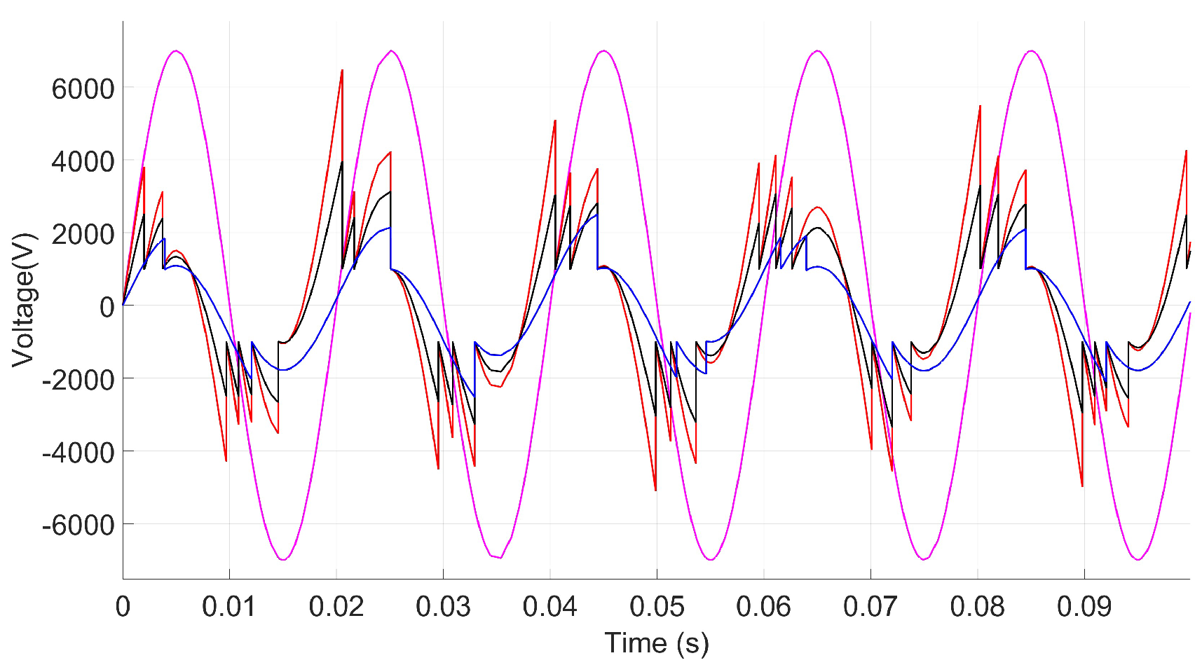
| Applied voltage | AC 7–11 kV, frequency: . |
| Ground | Negative electrode grounded at . |
| Parameter | Description |
|---|---|
| Inception voltage | . |
| PD current | Integrated the current density over ground boundaries. |
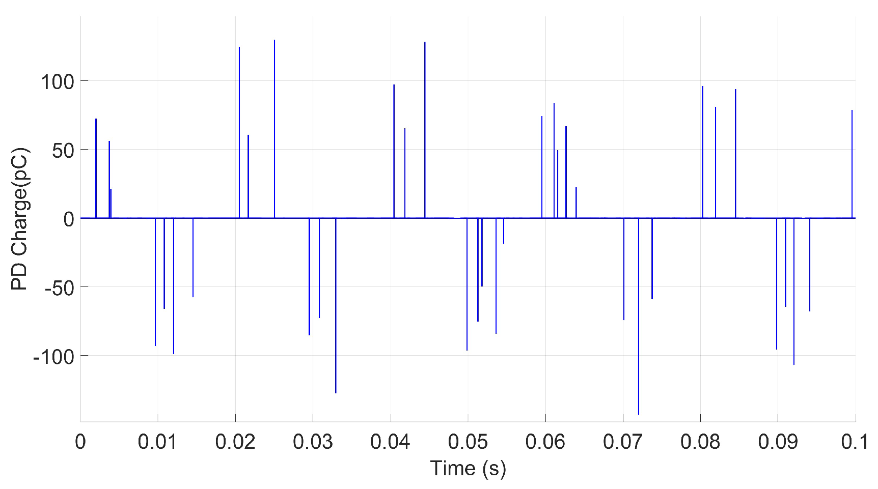
| Surface charge density | Integrated over cavity boundaries. |
| Space charge density | Computed within the cavity domain. |
| Time steps | With 1 ns during PD events and 1 μs otherwise. |
 |
| Parameter | Value |
|---|---|
| Optimizer | Adam |
| Initial learning rate | |
| Batch size | 64 |
| Epochs | 80 |
| Learning rate schedule | Step decay (factor = 0.1 every 20 epochs) |
| Weight initialization | ImageNet pretrained |
| Data augmentation | Random horizontal flip |
| Method | Dataset | Accuracy | Precision | Recall | F1-Score | AUC |
|---|---|---|---|---|---|---|
| STFT | Simulation | 90.00% | 0.91 (D) 1.00 (S) 0.83 (T) | 1.00 (D) 0.70 (S) 1.00 (T) | 0.895 | – |
| Experiment | 75.00% | 75.25% | 75.00% | 74.94% | – | |
| WT | Simulation | 93.33% | 0.90 (D) 0.90 (S) 1.00 (T) | 0.90 (D) 0.90 (S) 1.00 (T) | 0.933 | – |
| Experiment | 85.00% | 85.35% | 85.00% | 84.96% | – | |
| WVD | Simulation | 93.33% | 0.95 (D) 0.95 (S) 0.91 (T) | 0.90 (D) 0.90 (S) 1.00 (T) | 0.933 | – |
| Experiment | 94.74% | 95.45% | 94.44% | 94.68% | 0.947 | |
| HHT | Simulation | 88.33% | 1.00 (D) 0.89 (S) 0.78 (T) | 0.90 (D) 0.85 (S) 0.90 (T) | 0.886 | – |
| Experiment | 70.00% | 73.81% | 70.00% | 68.75% | – | |
| FRWT | Simulation | 95.00% | 1.00 (D) 0.95 (S) 0.91 (T) | 0.90 (D) 0.95 (S) 1.00 (T) | 0.950 | – |
| Experiment | – | – | – | – | – | |
| SWT | Simulation | 96.67% | 1.00 (D) 0.91 (S) 1.00 (T) | 0.90 (D) 1.00 (S) 1.00 (T) | 0.967 | – |
| Experiment | 100.00% | 100.00% | 100.00% | 100.00% | 1.000 |
| Method | Accuracy Drop |
|---|---|
| STFT | 15.00% |
| HHT | 18.33% |
| Method | Simulation Confusion Matrix | Experimental Confusion Matrix |
|---|---|---|
| Short-Time Fourier Transform (STFT) |  |  |
| Wavelet Transform (WT) |  |  |
| Wigner–Ville Distribution (WVD) |  | 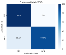 |
| Hilbert–Huang Transform (HHT) |  |  |
| Scatter Wavelet Transform (SWT) |  | 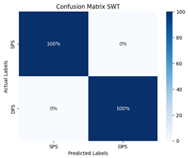 |
Disclaimer/Publisher’s Note: The statements, opinions and data contained in all publications are solely those of the individual author(s) and contributor(s) and not of MDPI and/or the editor(s). MDPI and/or the editor(s) disclaim responsibility for any injury to people or property resulting from any ideas, methods, instructions or products referred to in the content. |
© 2025 by the authors. Licensee MDPI, Basel, Switzerland. This article is an open access article distributed under the terms and conditions of the Creative Commons Attribution (CC BY) license (https://creativecommons.org/licenses/by/4.0/).
Share and Cite
Almehdhar, A.; Prochazka, R. Classification of Multiple Partial Discharge Sources Using Time-Frequency Analysis and Deep Learning. Appl. Sci. 2025, 15, 5455. https://doi.org/10.3390/app15105455
Almehdhar A, Prochazka R. Classification of Multiple Partial Discharge Sources Using Time-Frequency Analysis and Deep Learning. Applied Sciences. 2025; 15(10):5455. https://doi.org/10.3390/app15105455
Chicago/Turabian StyleAlmehdhar, Awad, and Radek Prochazka. 2025. "Classification of Multiple Partial Discharge Sources Using Time-Frequency Analysis and Deep Learning" Applied Sciences 15, no. 10: 5455. https://doi.org/10.3390/app15105455
APA StyleAlmehdhar, A., & Prochazka, R. (2025). Classification of Multiple Partial Discharge Sources Using Time-Frequency Analysis and Deep Learning. Applied Sciences, 15(10), 5455. https://doi.org/10.3390/app15105455