A Traffic Information Detection Method at Single Intersection Based on Wi-Fi Data

Abstract

Traffic information analysis plays an essential role in urban signalized intersection control. Wi-Fi technology can be used in multiple scenarios. It is effective to use a Wi-Fi data acquisition device to detect traffic information. This paper aims to study a traffic information detection method at a single intersection based on Wi-Fi data, determine the architecture design of the Wi-Fi data acquisition system, design the Wi-Fi data processing process, and then realize the acquisition of Wi-Fi data at a single intersection. K-means clustering algorithms and the LSTM neural network prediction model are used to obtain the space mean speed and vehicle steering ratio of the intersection sections. This method can be used to obtain and forecast various types of traffic information at intersections. The traffic information of an intersection in Xi’an is detected and predicted by using Wi-Fi technology. The experimental results show that the proposed method has high prediction accuracy.

1. Introduction

Intersections are bottleneck areas in urban road networks. Affected by the surrounding environment, pedestrians, and other complex factors, urban road intersections are prone to problems such as congestion and delay, which spread to the surrounding urban road network and seriously affect people’s daily commuting.

Addressing urban traffic challenges hinges on optimizing intersection performance. Traffic signal control plays a vital role by allocating right-of-way to conflicting traffic streams that cannot be spatially separated, thus managing their movement through time-based sequencing. Effective signal control strategies can dynamically adjust capacity in response to real-time traffic fluctuations, enhancing safety and efficiency while maximizing benefits for all road users [1,2].

The accurate and timely acquisition of traffic information is the premise of optimizing intersection signal control schemes and alleviating traffic problems. Currently, there are several ways to obtain traffic information. Zhang et al. introduced an attention mechanism to capture the relationship between the importance distribution and the duration of historical time series to predict the traffic flow at intersections [3]. Xu et al. proposed a deep-learning model based on Signal-control Refined Dynamic Traffic Graph (ScR-DTG) to predict the traffic volume of upcoming intersection movements [4]. Azimjonov Jahongir et al. developed a vision-based real-time traffic flow monitoring system to calculate traffic flow information such as vehicle direction, total number, instantaneous speed, and average speed based on the predicted trajectory [5]. Yue et al. proposed a method based on image fusion for detecting traffic objects under low light conditions [6]. Liu et al. proposed a method for traffic information detection based on satellite images [7]. Guo et al. proposed an improved wavelet transform to detect the singularities of real-time traffic flow signals, which can predict traffic flow with higher prediction accuracy and lower computation cost [8]. Liu et al. proposed a millimeter-wave radar for traffic flow detection, which can realize traffic behavior analysis and traffic flow parameter identification [9]. Huang et al. proposed a new traffic flow prediction approach from the perspective of vehicle functions by using radio frequency identification (RFID) electronic license plate (ELP) data [10]. Bhargava Kushagra et al. built geo-reference locations for dynamic cooperative communication, simulated mixed traffic and connected vehicle traffic flow scenarios, and analyzed the improvement of commute time, queue, and congestion [11].

Wi-Fi data acquisition technology has high accuracy and strong adaptability in a small range and is almost unaffected by weather and road environments [12]. Owing to its short propagation distance and fast propagation attenuation, Wi-Fi is suitable for positioning based on the Received Signal Strength (RSS) [13]. Most urban residents’ mobile phones, personal computers, and other mobile devices support Wi-Fi technology, and daily work and entertainment also focus on using Wi-Fi to connect to the internet. According to relevant statistics, 40% of mobile device users forget to turn off the Wi-Fi function after enabling it [14]. The combination of Wi-Fi positioning and spatiotemporal correlation analysis promotes the application of Wi-Fi data acquisition technology in various scenarios.

Currently, the research and application of Wi-Fi data acquisition technology are relatively extensive, and there are many applications and deployments in buildings or public places. Thor S. Prentow et al. used a large number of network Wi-Fi data analyses to extract personnel activity trajectories. This approach can provide better data support for facility management and planning activities in large buildings [15]. Mathieu Cunche studied privacy problems for owners of wireless portable devices and how to address potential risks [16]. Arief Hidayat et al. used Wi-Fi technology to collect non-passenger data on pedestrians, vehicles, and buildings in cities. The collected results were displayed on the map as reference data for travel [17]. Xu et al. designed a pedestrian pressure monitoring system using Wi-Fi technology and positioning based on Received Signal Strength Indicator (RSSI) [18]. Zhao et al. proposed a positioning and tracking scheme based on Wi-Fi location big data to obtain a target’s usual location through statistical analysis [19]. Huang et al. proposed a distance-based outdoor pedestrian positioning method using Wi-Fi to estimate high-precision distance [20].

Wi-Fi has also been used to detect vehicle paths. The authors in [21] studied the Wi-Fi patrol line obstacle avoidance car. The research aimed to improve the quality of people’s daily lives and play a cornerstone role in automatic driving and cargo transportation in terms of intelligent vehicle environment detection technology. The authors in [22] proposed an approach to industrial vehicle flow analysis to improve factory transportation management. The efficiency of internal logistics was improved with the Wi-Fi-based technique for monitoring industrial vehicles. The authors in [23] proposed an intelligent parking management system based on Wi-Fi positioning and Bluetooth control technologies to manage vehicles entering or exiting a parking lot. Owing to its convenience, practicability, and low cost, such a parking system using Bluetooth identification based on Wi-Fi positioning was worth popularizing. The authors in [24] described an approach to monitoring pedestrian and vehicle activities in outdoor urban environments based on the analysis of wireless probe requests. Load tests demonstrated a sensor’s ability to maintain a probe request capture rate above 95% over a wide range of probe request emission rates.

Wi-Fi data technology can be further applied to the traffic field by linking individual movement behavior with traffic commute behavior. The authors in [25] measured bus passenger load by detecting the periodic network detection activity of Wi-Fi devices in “smartphones” and concluded that Wi-Fi activity was indeed correlated with passenger flow. The authors in [26,27] estimated the number of bus passengers based on the Wi-Fi data survey and the extracted passenger volume data. The authors in [28] proposed the construction concept of “a traffic network detection platform based on Bluetooth and Wi-Fi wireless technologies”, which can detect vehicle speed through wireless devices. The detection accuracy of this platform reached 85–90%. The authors in [29] used Wi-Fi data acquisition technology to estimate the occupancy rate of public transportation and analyzed the operational efficiency of bus lines based on it. The authors in [30] designed and implemented a traffic flow monitoring system based on Wi-Fi data acquisition technology, which performed well in road sections with a relatively simple environment. The authors in [31] deployed Wi-Fi data acquisition devices on buses, used the maximum expectation algorithm to screen bus passengers effectively, and conducted a preliminary study on public transport passenger flow estimation. The authors in [32] used Wi-Fi services provided on buses to estimate real-time urban traffic conditions and verified that Wi-Fi data collection technology in urban areas was an excellent supplement to existing traffic conditions collection.

In the above studies, Wi-Fi data acquisition technology has primarily been applied to relatively straightforward scenarios, such as public transportation systems, where travel behaviors are straightforward and traffic information exhibits high substitutability. As a result, its broader applications remain limited. However, given the increasing complexity of urban road networks and the growing diversity of commuter behaviors, Wi-Fi data acquisition holds significant untapped potential for more advanced traffic management and analysis.

This study proposes a traffic information detection method at a single intersection based on Wi-Fi data. The method tracks the vehicle trajectory through the Wi-Fi data MAC address so as to realize the space mean speed and vehicle steering ratio detection at the intersection entrance. Compared to traditional detection technology, this method can expand the type of conventional traffic information detection. The use of a Wi-Fi data MAC address as a track label has a higher penetration rate than satellite positioning technology, and the track positioning accuracy is higher than that of mobile signaling data [33,34]. The detection accuracy of traffic information was greatly improved [35,36]. The detection device is cheap and easy to install and maintain. The original data format is simple and can quickly be processed and stored. The detection targets are various. The detection device is convenient for networking and has a comprehensive detection range.

The rest of this study is organized as follows: Section 2 summarizes the proposed method’s system framework and key techniques. In Section 3, the traffic information collection process is given, and the prediction model is established. In Section 4, the prediction model is verified and evaluated. Finally, a conclusion is drawn in Section 5.

2. Theoretical and Technical Foundations

The realization of this system is based on the collection of Wi-Fi data at a single intersection. If the Wi-Fi collection device is rationally arranged at the intersection, the Wi-Fi data of the mobile devices carried by the passengers in the vehicle on the road can be collected, and the traffic information of the intersection can be further detected.

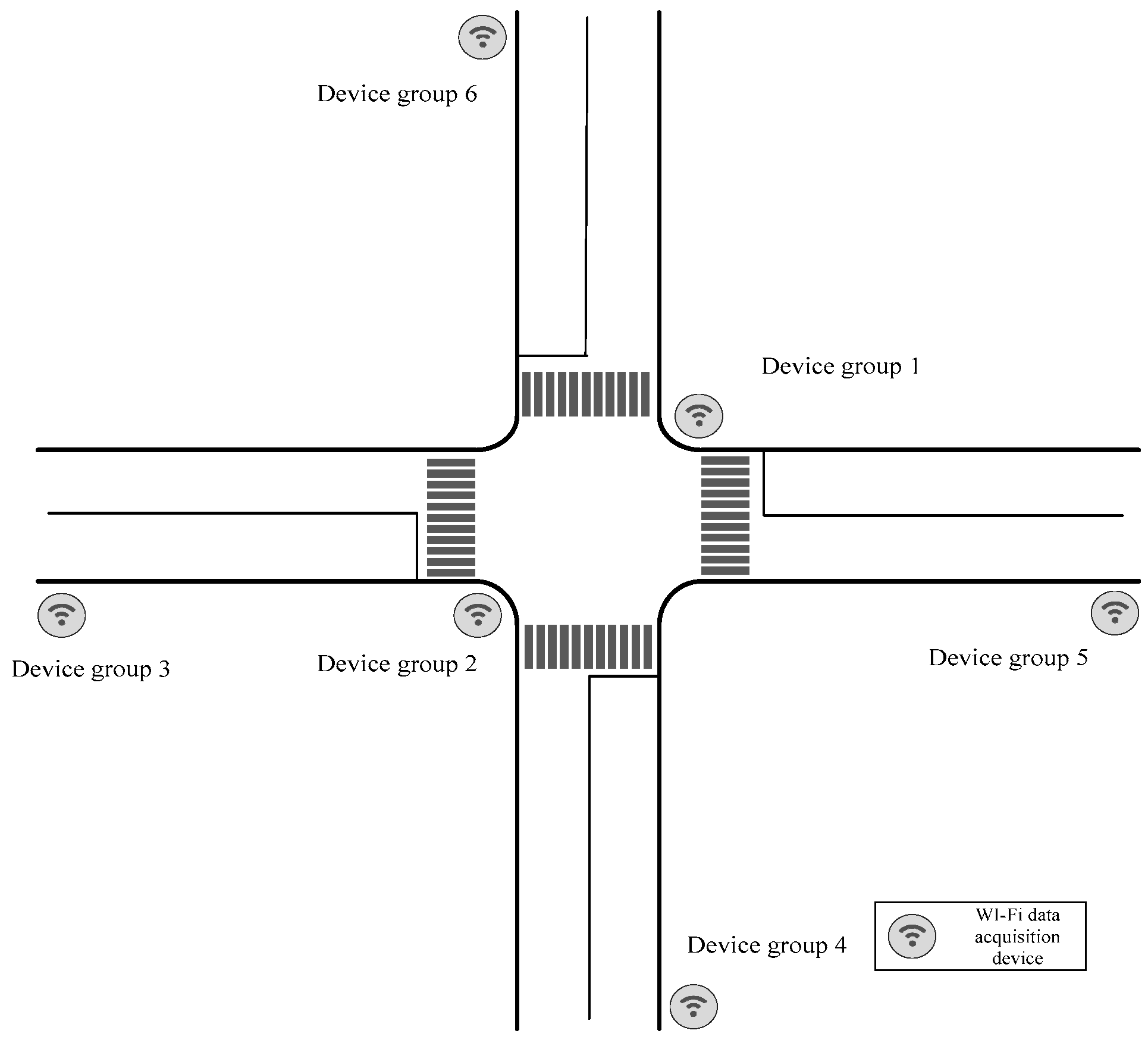
2.1. System Architecture of Wi-Fi Data Acquisition

The system architecture is shown in Figure 1, and mainly includes the Wi-Fi data acquisition module, data upload module, and background servers. The Wi-Fi data acquisition module uses a TZ Wi-Fi probe. The data upload module uses commercially available mobile hotspot devices to provide Wi-Fi probes with the network required for data upload in various scenarios and ensures the time synchronization of different probe devices. The background server is an efficient and stable Ali Cloud server that can meet the needs of multiple Wi-Fi collection devices to upload data simultaneously. The proposed devices do not require calibration. The primary role of wireless devices is to detect time and estimate location, which are achieved through algorithms.

2.2. Key Technology

2.2.1. MAC Address Matching

The MAC address of the device network card is assigned by the IEEE and is unique worldwide. MAC address matching compares the MAC address traversal in the Wi-Fi data sets of two different acquisition points and finds the MAC address that appears in both Wi-Fi data sets simultaneously. This is the MAC address matching of Wi-Fi data [37]. After MAC address matching, the spatial-temporal correlation information in the Wi-Fi data can be analyzed based on the corresponding detection timestamp and the actual location of the collection point.

2.2.2. K-Means Clustering

This method still maintains high efficiency and scalability when processing extensive data. Due to its simplicity and speed, this method is effective for recognizing urban cross-traffic information [38].

The common performance indicators of clustering algorithms are the sum of squared error (SSE) and the silhouette coefficient. The sum of the squares errors is an important objective function in the iteration of the clustering algorithm, and can directly reflect the quality of the clustering effect, as in (1). The smaller the sum of squares error, the better the clustering effect. Generally, the sum of squares error gradually decreases with an increase in the number of clusters, but blindly increasing the number of clusters increases the computational complexity.

The average silhouette coefficient is the average value of the silhouette coefficient of all samples in the clustering process, which can fully reflect the degree of cohesion and separation of each sample in the clustering result, as shown in (2). The value interval of the average silhouette coefficient is [−1, 1]. The larger the value, the better the result. When the value is close to zero, the clustering result samples overlap. A negative value indicates that a large number of samples are assigned to clusters that do not meet the expectations.

$$SSE=\sum _{i=1}^K\sum _{pϵC_i}|p-m_i{|}^2$$

(1)

Among them, K is the specified initial cluster number, Ci is the ith cluster, $p$ is the sample point in Ci, and $m_i$ is the central point in Ci.

$$\overline{S}=\sum _{i=1}^n{\displaystyle \frac{b_i-a_i}{\mathrm{m}\mathrm{a}\mathrm{x}\left(a_i,b_i\right)}}/n$$

(2)

where $\overline{S}$ is the average silhouette coefficient and $n$ is the number of cluster samples. $a_i$ is the average Euclidean distance between the ith sample and other samples in the same cluster, which reflects the cohesion of the sample. $b_i$ is the average Euclidean distance between the ith sample and other samples in different clusters, which reflects the separation degree of the sample.

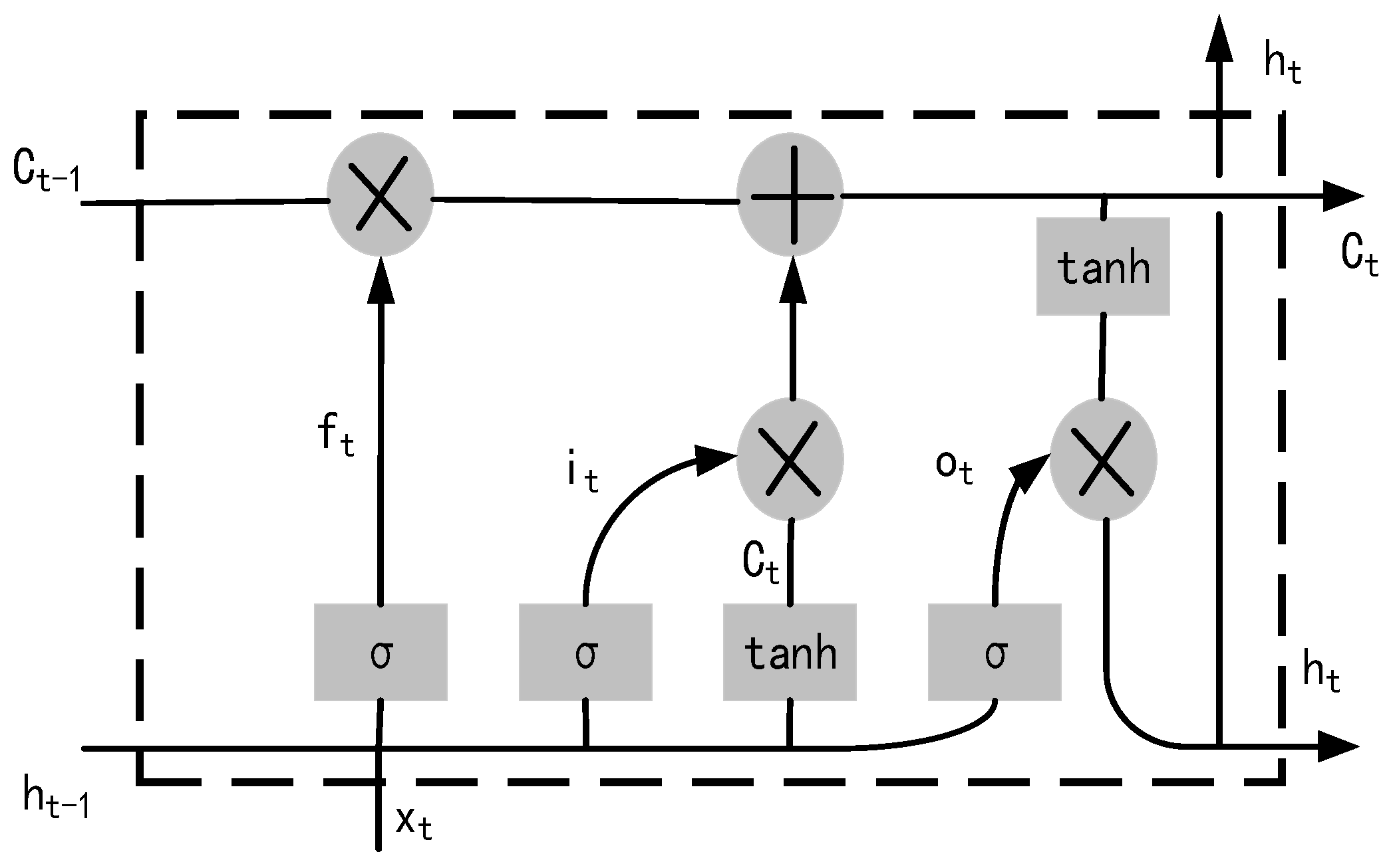
2.2.3. LSTM Neural Network Model

The special gate structure of the LSTM neural network model enables it to remember or forget long-term information selectively. It has significant advantages in time series prediction. The traffic information data of intersections are time series data with a spatial-temporal correlation. Hence, the LSTM neural network model is suitable for predicting the traffic information data.

The typical LSTM neural network model structure is shown in Figure 2. Among them, the function of the forgetting gate is to use the sigmoid function to retain the cell state information of the previous moment selectively, and its input is the input information $x_t$ of the current moment and the hidden layer information $h_{t-1}$ of the previous moment, as in (3). The function of the input gate is to obtain the candidate cell state information ${\tilde{C}}_t$ by using the tanh function and update the cell state information $C_t$ at this moment by combining the cell state information $C_{t-1}$ at the previous moment, as in (4). The output gate calculates the final output information $h_t$ and determines $C_t$, $x_t$, and $h_{t-1}$ when the information can be passed to the next time. The final output information $h_t$ is calculated in (5).

$$f_t=\sigma \left(W_f\cdot \left[h_{t-1},x_t\right]+b_f\right)$$

(3)

$$\begin{gathered} i_t=\sigma \left(W_i\cdot \left[h_{t-1},x_t\right]+b_i\right) \\ {\tilde{C}}_t=\mathrm{t}\mathrm{a}\mathrm{n}\mathrm{h}\left(W_c\cdot \left[h_{t-1},x_t\right]+b_c\right) \\ {C}_t=f_t\cdot C_{t-1}+i_t\cdot {\tilde{C}}_t \end{gathered}$$

(4)

$$\begin{gathered} o_t=\sigma \left(W_o\left[h_{t-1},x_t\right]+b_o\right) \\ {h}_t=o_t\cdot \mathrm{t}\mathrm{a}\mathrm{n}\mathrm{h}\left(C_t\right) \end{gathered}$$

(5)

3. Methodology

This section further studies the process of processing Wi-Fi data into traffic information and proposes a traffic information detection method for intersections based on Wi-Fi data. The detection process of traffic information is first presented, followed by the Wi-Fi data preprocessing process. Next, the calculation method of the spatial average speed of the intersection and the vehicle turning ratio information is introduced. Finally, the traffic data prediction model of the entrance section of the intersection is given.

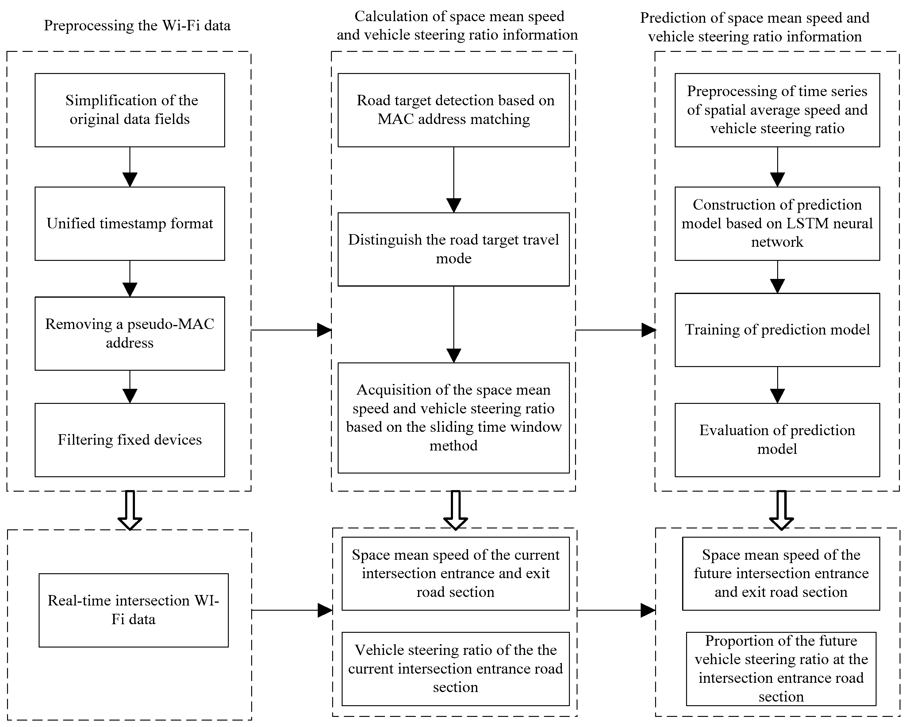
3.1. Traffic Information Detection Process

The traffic information detection method based on Wi-Fi data is shown in Figure 3. Firstly, the Wi-Fi data preprocessing process is designed. Secondly, the calculation process of the space mean speed of the road section and the vehicle steering ratio information of the road entrance section is designed. Then, the traffic information prediction model of the road entrance section based on the LSTM network is constructed to achieve the prediction of the space mean speed and the vehicle steering ratio.

3.2. Preprocessing the Wi-Fi Data

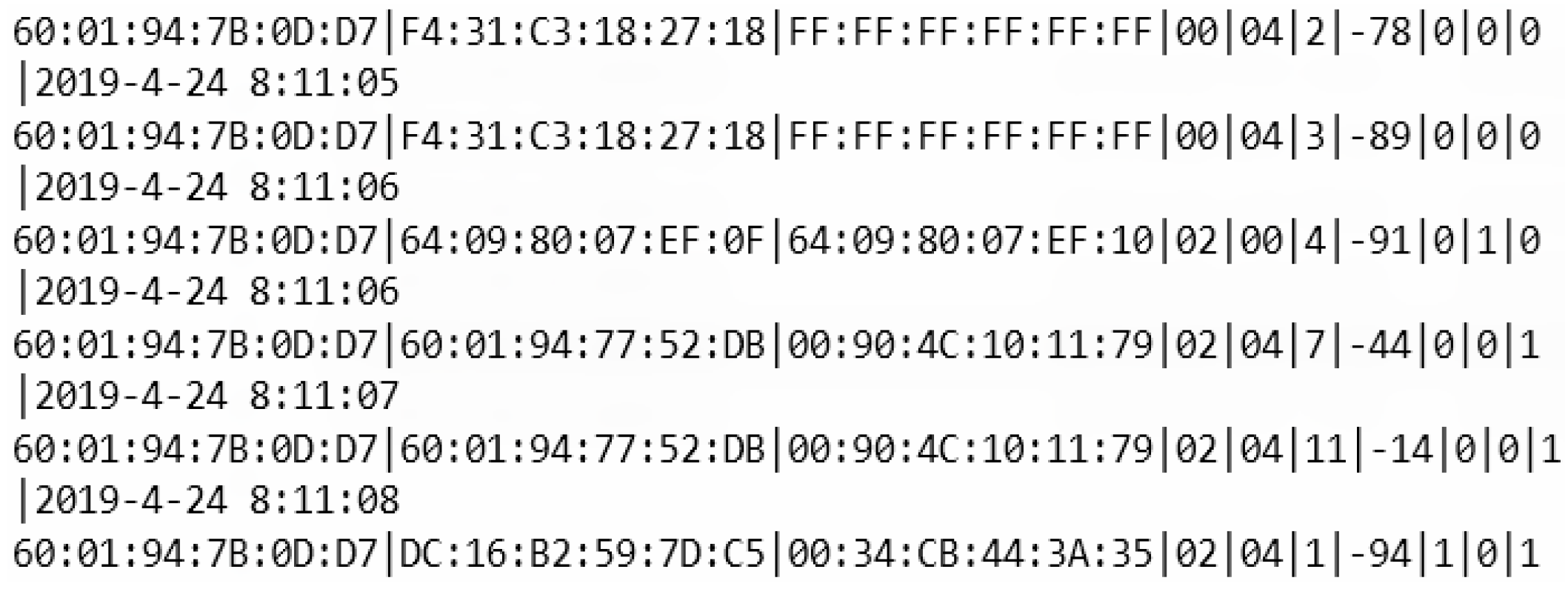
3.2.1. Simplification of the Original Data Fields

The original Wi-Fi data are sent by character stream. The raw data collected by Wi-Fi contain the following fields: probe device MAC, source MAC, destination MAC, frame main type, frame subtype, scan channel, signal strength RSS, and timestamp. Examples of raw Wi-Fi data are shown in Figure 4. The specific meanings of each field in the data are as follows: Probe MAC, which is the MAC address of the Wi-Fi module of the probe itself, mainly used for distinguishing different probes; source MAC, which is the MAC address of the transmitting end of the Wi-Fi signal collected by the probe, mainly for mobile devices; destination MAC, which is the MAC address of the receiving end of the Wi-Fi signal collected by the probe, possibly for mobile devices or fixed devices; frame type, which is one of the values “00”, “01”, and “02”, corresponding to management frames, control frames, and data frames, respectively; frame sub-type, which is the sub-type of the Wi-Fi signal frame collected by the probe under different main types; scan channel, which is the specific communication frequency band where the Wi-Fi signal is located; signal strength, which is the strength of the Wi-Fi signal collected by the probe, with the minimum value being −100; the larger this value is larger, the stronger the signal strength is, and the closer the Wi-Fi signal transmitting device is to the probe; timestamp, which is the moment when the Wi-Fi data are collected.

In order to take into account the data necessary for the subsequent algorithm, the method only retains the source MAC address, detected timestamp, and signal strength.

3.2.2. Unified Timestamp Format

The timestamp is the key data required for obtaining traffic information at intersections. In practice, a large number of acquisition devices are used on-site, and the batches of the devices are inconsistent, which will lead to inconsistent timestamp formats. Therefore, the timestamp format is set to yyyy/MM/dd hh:mm:ss to ensure efficiency and accuracy in subsequent data processing.

3.2.3. Removing a Pseudo-MAC Address

A few mobile device manufacturers use random MAC address technology to protect user privacy. This way, there are few rules to follow and affect the subsequent traffic information. The second hexadecimal character of an actual MAC address can only be “0”, “4”, “8”, or “c”. Based on this rule, pseudo-MAC addresses can be effectively removed.

3.2.4. Filtering Fixed Devices

The raw data may include Wi-Fi data transmitted by fixed devices in places such as shops and office buildings around roads in the actual environment. Two rules are used to filter fixed equipment during the preprocessing process. First, the method is based on the MAC address vendor data set published by IEEE, matches the corresponding MAC address brands, and removes MAC addresses that do not belong to mainstream mobile device brands. Second, the method removes MAC addresses that appear at a collection point and are continuously collected for over one hour.

Table 1. Examples of preprocessed data.

MAC Addresses	Timestamp	RSS
50:XX:55:0F:F9:00	2019.4.24 08:25:01	−87
78:XX:51:07:1E:19	2019.4.24 08:25:01	−85
F0:XX:98:12:47:B5	2019.4.24 08:50:33	−44
94:XX:29:7E:92:FD	2019.4.24 09:52:06	−75
B4:XX:44:EB:B6:0F	2019.4.24 12:20:26	−7
1C:XX:CE:53:1E:23	2019.4.24 12:32:34	−90
D4:XX:3F:46:68:67	2019.4.24 15:53:45	−94
00:XX:4C:10:11:82	2019.4.24 08:50:56	−39

shows examples of the preprocessed data format (MAC addresses in the table have been privatized). Each piece of Wi-Fi data contains the MAC address of the Wi-Fi data corresponding to the source device, the timestamp of the Wi-Fi data, and the Wi-Fi signal strength RSS of the Wi-Fi data corresponding to the source device.

3.3. Calculation of Intersection Data

After the original Wi-Fi data are preprocessed in real-time, the inherent spatiotemporal information of the Wi-Fi data at the intersection can be further mined so that the space mean speed and vehicle steering ratio information of the entrance and exit sections of a single intersection can be calculated.

3.3.1. Road Target Detection Based on MAC Address Matching

The road target detected based on Wi-Fi data is defined as follows: the target passes through the Wi-Fi data collection points, including the upstream, crossing, and downstream of the intersection successively within a reasonable time range (the upstream and downstream here depend on the road target running track). All three collection sites were able to detect Wi-Fi signals from the target.

The data collected by multiple device groups located at each collection point around the intersection are fused. ${data}_o$ is the Wi-Fi data set of the intersection collection point. ${data}_e,{data}_w,{data}_s,$ and ${data}_n$ are the Wi-Fi data sets of the four adjacent sections around the intersection in the east, west, south, and north directions. Taking the detection of road targets passing through the intersection from east to west as an example, the specific steps of the MAC address matching algorithm for Wi-Fi data at a single intersection are as follows:

Step 1: The MAC address set that has not appeared for three consecutive minutes at the $\mathrm{t}$ minute in the data set ${\mathrm{d}\mathrm{a}\mathrm{t}\mathrm{a}}_{\mathrm{o}}$ is found in chronological order and is denoted as $M$.

Step 2: Wi-Fi data set ${data}_e^t$ within the minutes from $t-13$ to $t-3$ is extracted in ${data}_e$, and Wi-Fi data set ${data}_w^t$ within the minutes from $t-3$ to $t+7$ is extracted in ${\mathrm{d}\mathrm{a}\mathrm{t}\mathrm{a}}_{\mathrm{w}}$.

Step 3: Iterate over the MAC addresses in the data set $M$. If the Wi-Fi data record corresponding to the MAC address can be found in ${data}_e^t$ and ${data}_w^t$, the target corresponding to the MAC address is the detected road target. Then, the timestamp corresponding to the maximum RSS (Wi-Fi signal strength) in the Wi-Fi data record of the collection point is regarded as the time when this road target passes through the location of the corresponding collection point.

Step 4: The road target and its related information constitute the road target data set, which is denoted as $obj-dataset$. The data set mainly includes the MAC address of the road target ${obj}_o$, the corresponding travel time $t_o^{in}$ of the entrance section when passing the intersection, the travel speed $v_o^{in}$ of the entrance section, the travel time $t_o^{out}$ of the exit section, the travel speed $v_o^{out}$ of the exit section, and the orientation of the upstream and downstream collection points. Add one and jump to step 1 after completing the traversal.

After MAC address matching, the road target ${obj}_o$ passes through the intersection, the timestamps $t_o^{st}$, $t_o^{ce},$ and $t_o^{ed}$ can be obtained when the target successively passes the data collection points upstream, crossing, and downstream of the intersection. Further, the travel time and travel speed of the road target passing through the entrance and exit sections of the intersection can be obtained by combining the actual location and relative distance of the collection point. The calculation is detailed in Formulas (6)–(9).

$$t_o^{in}=t_o^{st}-t_o^{ce}$$

(6)

$$t_o^{out}=t_o^{ce}-t_o^{ed}$$

(7)

$$v_o^{in}=d^{st}/t_o^{in}$$

(8)

$$v_o^{out}=d^{ed}/t_o^{out}$$

(9)

where $t_o^{in}$ and $t_o^{out}$ are the travel time of the entrance and exit sections of the intersection road target, respectively, $v_o^{in}$ and $v_o^{out}$ are the travel speed of the entrance section and the exit section, and $d^{st }$ and $d^{ed}$ are the actual distances between the upstream and downstream data collection points and the intersection data collection points, respectively. The st stands for the region upstream of the intersection. The ce stands for the intersection. The ed stands for the region downstream of the intersection.

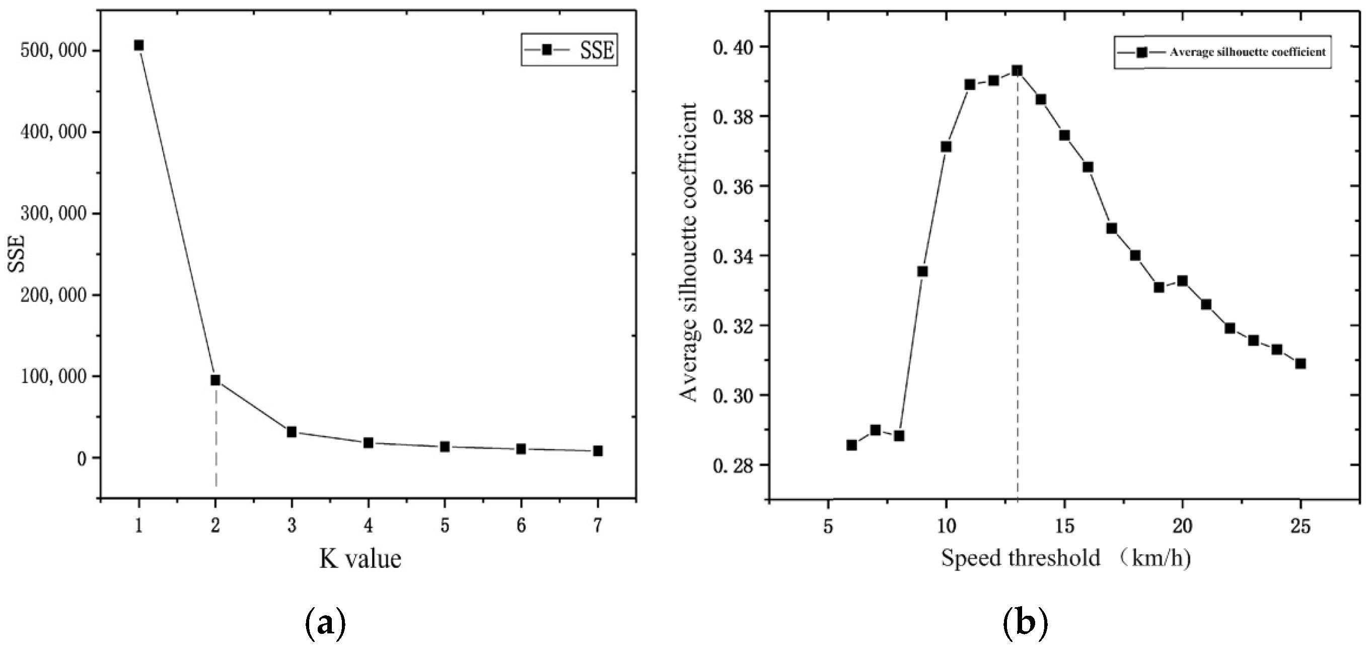
3.3.2. Distinguish the Road Target Travel Mode

The K-means clustering algorithm is selected to distinguish the travel modes of the road targets. Pedestrian and non-motor vehicle speeds are low, generally distributed below 10 km/h, and there is a big difference with motor vehicles. During peak traffic periods, intersections are congested, and vehicles queue up for a long time. The speed of pedestrians and non-motor vehicles less affected by congestion may exceed that of motor vehicles, but the speed difference of pedestrians and non-motor vehicles through the intersection is not significant. Therefore, the travel speed of the entrance section, the travel speed of the exit section, and the travel speed difference between the entrance section and the exit section of the road target are selected as the clustering characteristics to distinguish the travel mode of the target. Firstly, the K-means algorithm is used to distinguish low-speed travel modes of walking and non-motor vehicle travel from motor vehicle travel. Secondly, the road target travel mode of motor vehicle travel is further divided into private car travel and public transport travel according to the spatial-temporal correlation analysis.

The specific steps of road target travel mode differentiation are as follows:

Step 1: Select the road target data set $obj-dataset$. For the road target sample ${obj}_o$ in the data set, the speed $v_o^{in}$ of the entrance section, the speed $v_o^{out}$ of the exit section, and the speed difference $v_o^{diff}$ of the entrance and exit section are obtained as the clustering feature. The $v_o^{diff}$ can be obtained as follows:

$$v_o^{diff}=|v_o^{in}-v_o^{out}|$$

(10)

Step 2: Determine the initial number of cluster centers $K$. The K value is determined using the elbow method. The reason is that the actual intersection traffic environment is complex, and it is a better way to determine the value $\mathrm{K}$ by using the internal correlation of the data set itself. The $K$ value corresponding to the obvious inflection point of the SSE value decline is selected as the clustering $K$ value.

Step 3: Profile the data set $obj-dataset$ and then adjust it. The MAC address matching range of the collected data is wide, the low-speed target is easy to miss the report, and the sample distribution among clusters is unbalanced, which leads to the deviation of the cluster center. In addition, the travel speed of the road target of motor vehicle travel is vastly different, the distribution range is wide, and the cohesion is not strong when clustering. The data set is preliminarily classified. When the travel speed of the entrance section or the travel speed of the exit section of the sample exceeds the motor vehicle speed threshold $v_{thr}$, its travel mode is directly marked as motor vehicle travel. When the adjusted average silhouette coefficient of the data set reaches its maximum value, it is the selected vehicle speed threshold $v_{thr}$.

Step 4: K-means clustering is performed on the remaining unlabeled samples in $obj-dataset$. The sample travel modes in the class with the largest central speed characteristic value after clustering are labeled as motor vehicle travel, and the rest are labeled as walking and non-motor vehicle travel.

Step 5: Add a bus attribute value of $N_{bus}$ to all samples in $obj-dataset$, indicating that the sample is the passenger of the $N_{bus}$ TH bus target found. When $N_{bus}$ is 0, it means that the sample travel mode is not bus. The samples of all travel modes in the data set are taken as a data set, denoted as $obj-{dataset}^{\prime }$, and the counting variable $\mathrm{m}$ is initialized as 1.

Step 6: For sample ${\mathrm{o}\mathrm{b}\mathrm{j}}_{\mathrm{x}}$, whose bus attribute value $N_{bus}$ is null in the data set $obj-{dataset}^{\prime }$, traverse other samples whose bus attribute value $N_{bus}$ is null in the data set. Compare the differences in the timestamps corresponding to the same collection point between the upstream, downstream, crossing of the intersection, and other samples. All samples ${obj}_x$ with timestamp differences of less than 3 s are placed in set $\mathrm{t}\mathrm{e}\mathrm{m}\mathrm{p}$. If the number of sets $\mathrm{t}\mathrm{e}\mathrm{m}\mathrm{p}$ individuals $n$ is less than 3, go to step 7. If the number of sets $\mathrm{t}\mathrm{e}\mathrm{m}\mathrm{p}$ individuals $n$ is not less than 3, go to step 8.

Step 7: Set the bus attribute value $N_{bus}$ of all samples in $\mathrm{t}\mathrm{e}\mathrm{m}\mathrm{p}$ to “0” and empty $\mathrm{t}\mathrm{e}\mathrm{m}\mathrm{p}$. If there are still samples with bus attribute value $N_{bus}$ being null in data set $obj-{dataset}^{\prime }$, go to step 6; otherwise, go to step 9.

Step 8: Set the bus attribute $N_{bus}$ value of all samples in $\mathrm{t}\mathrm{e}\mathrm{m}\mathrm{p}$ to $m$, $m$ plus 1, and empty $\mathrm{t}\mathrm{e}\mathrm{m}\mathrm{p}$. If there are still samples in data set $obj-{dataset}^{\prime }$ for which the bus cattribute value $N_{bus}$ is null, go to step 6; otherwise, go to step 9.

Step 9: Set the attribute value of the sample whose bus attribute value is null in the data set $obj-dataset$ to “0.” The algorithm process is over. The road objectives of private car travel, public transport travel, and walking non-motor vehicle travel are recorded as ${obj}_i$, ${obj}_j$, and ${obj}_k$, respectively.

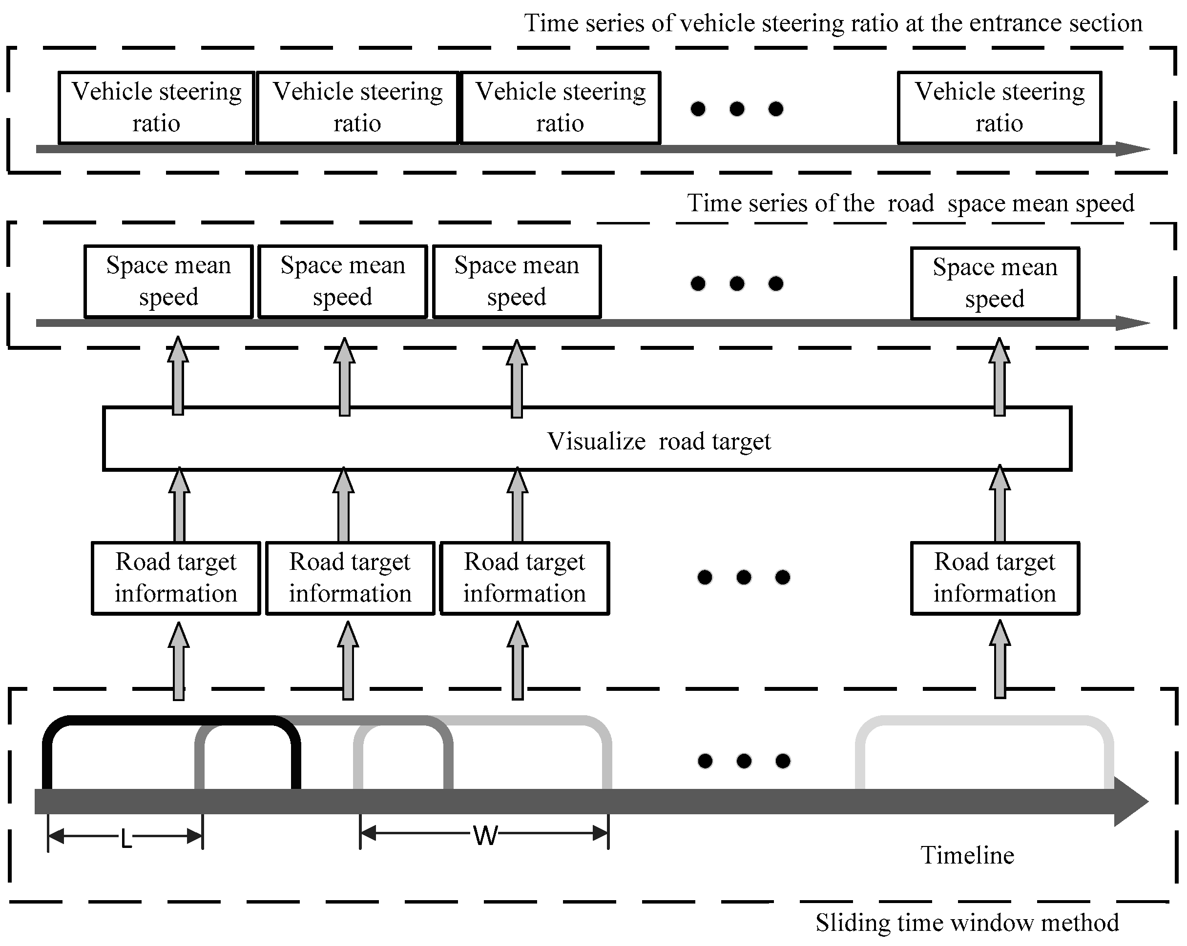
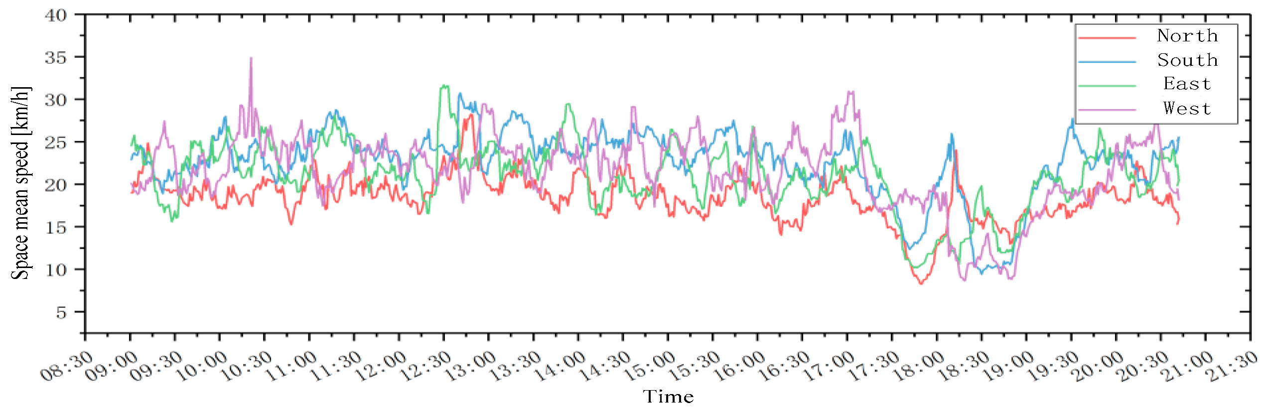
3.3.3. Calculation of Intersection Space Mean Speed and Vehicle Steering Ratio

The sliding time window method is used to further calculate the space mean speed of the road entrance and exit section and the vehicle steering ratio of the road entrance section. The width of the sliding time window is $w$, and the sliding step length is $l$. Each time window contains the road target, and its speed information detected after Wi-Fi data processing. The sliding time window method is shown in Figure 5.

The research object of this study is the intersection vehicle target. The road target in the time window needs to be visualized as a vehicle target, as follows: Removing the road target that the travel modes are walking or by a non-motor vehicle. The road targets traveling on the same public vehicle are aggregated and visualized into a bus, whose speed information is the average of the corresponding speed information of each road target. The road target of traveling by private car is directly visualized as a vehicle.

The visualization of the road target is equivalent to a random sampling of all vehicles passing through the intersection in that time period. Therefore, the harmonic average of the travel speed of vehicles after visualization in the time window can be approximated to the real space mean speed of the corresponding section, as in (11)–(13). Similarly, the vehicle steering ratio after the visualization of each entrance section can also be approximated to the actual vehicle steering ratio of the corresponding road section, as in (14) and (15).

$$V^t=1/\left(\sum _{i=1}^{N_{car}} \left(1/v_{car}\right)+\sum _{bus=1}^{N_{bus}} \left(1/v_{bus}\right)\right)$$

(11)

$$v_{bus}=\left(\sum _{j=1}^n{v}_j\right)/n$$

(12)

$$v_{car}=v_i$$

(13)

where $V^t$ is the space mean speed of each entrance and exit section of the intersection in the $\mathrm{t}$ time period, $N_{car}$ and $N_{bus}$ are, respectively, the number of private cars and buses passing through the section after Wi-Fi data processing and visualization in this time period, $v_i$ is the travel speed of the road target ${obj}_i$ for private car travel in this section, $v_{car}$ is the travel speed of the private vehicle after the visualization of ${obj}_i$, $v_j$ is the travel speed of $\mathrm{n}$ road targets ${obj}_j$ traveling by the same bus in this section, and $v_{bus}$ is the travel speed of bus vehicles after ${obj}_j$ concretion.

$$B^t=\left[b_L^t,b_T^t,b_R^t\right]=\left[{\displaystyle \frac{n_L}{N}},{\displaystyle \frac{n_T}{N}},{\displaystyle \frac{n_R}{N}}\right]$$

(14)

$$N=N_{car}+N_{bus}$$

(15)

where Bt is the vehicle steering ratio matrix of each entrance section in the $t$ time period. $b_L^t$, $b_T^t,$ and $b_R^t$ are the proportions of vehicles turning left, straight, and right on the road entrance section, respectively. $N$ is the number of all vehicles passing through the section after Wi-Fi data processing and visualization within the time period. Respectively, $n_L$, $n_T,$ and $n_R$ are the number of left turns, straight, and right turns in the above vehicles. N_bus is the total number of buses passing through the section after Wi-Fi data processing and visualization in a time period.

Considering the sampling rate of Wi-Fi data and subsequent traffic information prediction, this study sets the width of the sliding time window as 15 min and the sliding step length as 15 min. With the movement of the time window, the space mean speed and the vehicle steering ratio of the entrance and exit sections can be gradually obtained.

3.4. Traffic Data Prediction Model of the Intersection Entrance Section

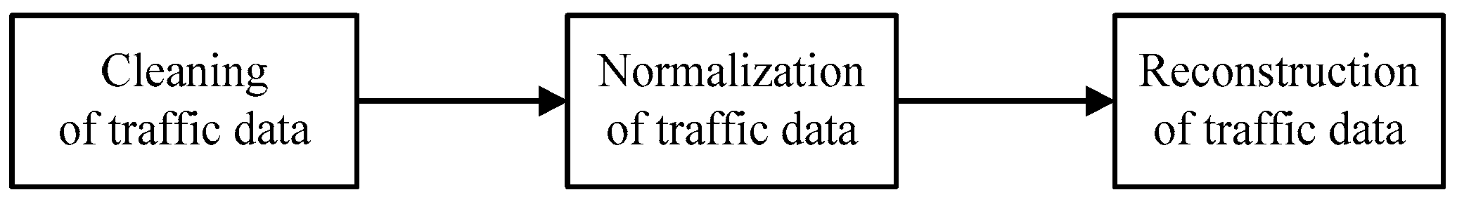
3.4.1. Training Data Preprocessing

The preprocessing of data has a significant impact on the prediction performance of the LSTM neural network model. Therefore, it is necessary to perform operations such as cleaning, normalization, and data reconstruction on the time series of traffic data obtained through Wi-Fi data processing. The flowchart of traffic data preprocessing is shown in Figure 6.

For the convenience of the following description, we will uniformly denote different types of traffic data as “x”. The specific steps for preprocessing traffic data are as follows.

Cleaning of traffic data:

(1)

When the traffic data represents the spatial average speed, the maximum value should be the highest speed limit of the road section. Speed data exceeding this maximum value and zero-value data should be marked as missing data.

(2)

When the traffic data are the vehicle steering ratio, the zero value data of the steering ratio should be marked as missing data. Finally, missing data in the time series are uniformly filled using the average of the adjacent data.

Normalization of traffic data:

(1)

When the traffic data are the spatial average speed, their values and fluctuation amplitudes are relatively large. The min–max method is adopted to normalize the speed data, which can reduce the size differences of the speed time series and accelerate the convergence process of LSTM neural network training, thereby improving the prediction effect.

(2)

When the traffic data are the vehicle steering ratio, no such operation is required.

Reconstruction of traffic data: The time series of the traffic data is reconstructed to obtain the training samples to reflect the temporal and spatial correlation of the samples. The time series data obtained from the Wi-Fi data processing has a period of 15 min, and the samples used for prediction are consistent with it. The sample format of traffic data obtained from time series reconstruction is shown in (16):

(1)

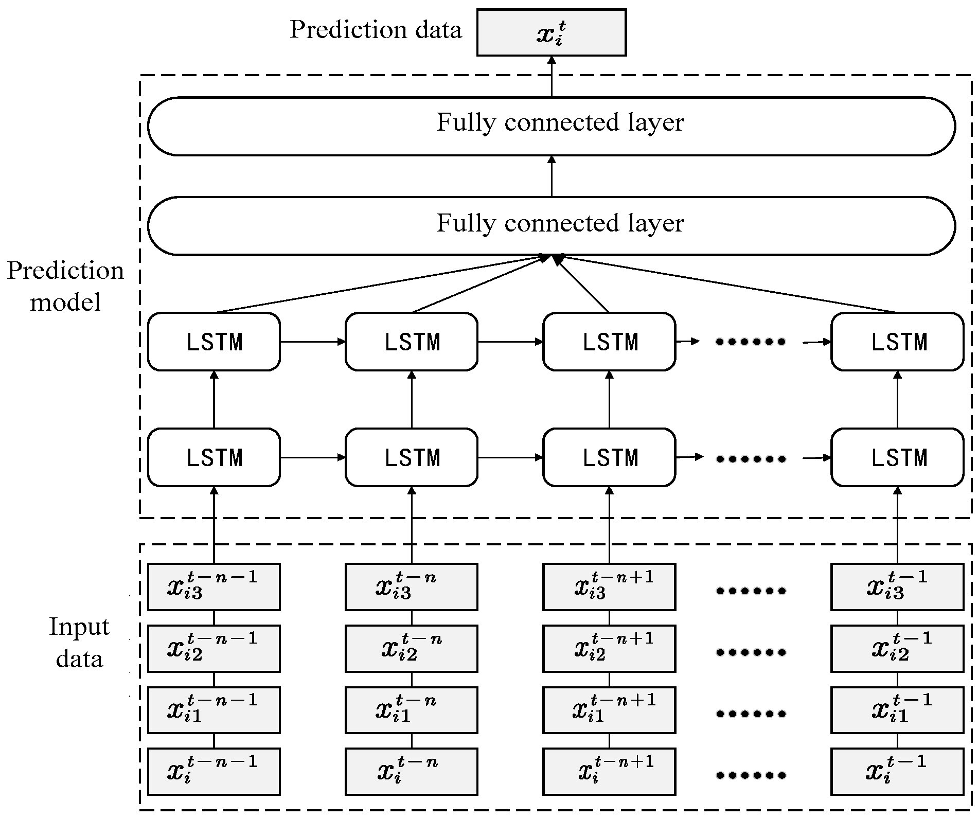
When the traffic data $x$ are the space mean speed, i is the number of the entrance section of the intersection that needs to be predicted in (16). $i1$, $i2$, and $i3$ are the numbers of the downstream left turn, straight, and right turn in intersection exit sections corresponding to the entrance section. The speed data of the entrance section and the three downstream exit sections, which include the current $t-1$ time period and the first $\mathrm{n}$ time period, are taken to predict the space mean speed $x_i^t$ of the entrance section $i$ in the future $t$ time period.

(2)

When the traffic data x are the vehicle steering ratio, i is the number of the entrance section of the intersection that needs to be predicted in (16). $i1$, $i2$, and $i3$ are the corresponding numbers of the other three road entrance sections, except the current road entrance section. The vehicle steering ratio data of the entrance itself and the other three entrance sections, including the input data of the current $t-1$ time period and the previous $n$ time period, are taken to predict the vehicle steering ratio $x_i^t$ of the entrance section $i$ in the future $t$ time period.

$$x_i^t=\left[\begin{array}{cccc}{x}_{i1}^{t-n-1}& .& .& x_{i1}^{t-1}\\ x_{i2}^{t-n-1}& .& .& x_{i2}^{t-1}\\ x_{i3}^{t-n-1}& .& .& x_{i3}^{t-1}\\ x_i^{t-n-1}& .& .& x_i^{t-1}\end{array}\right]$$

(16)

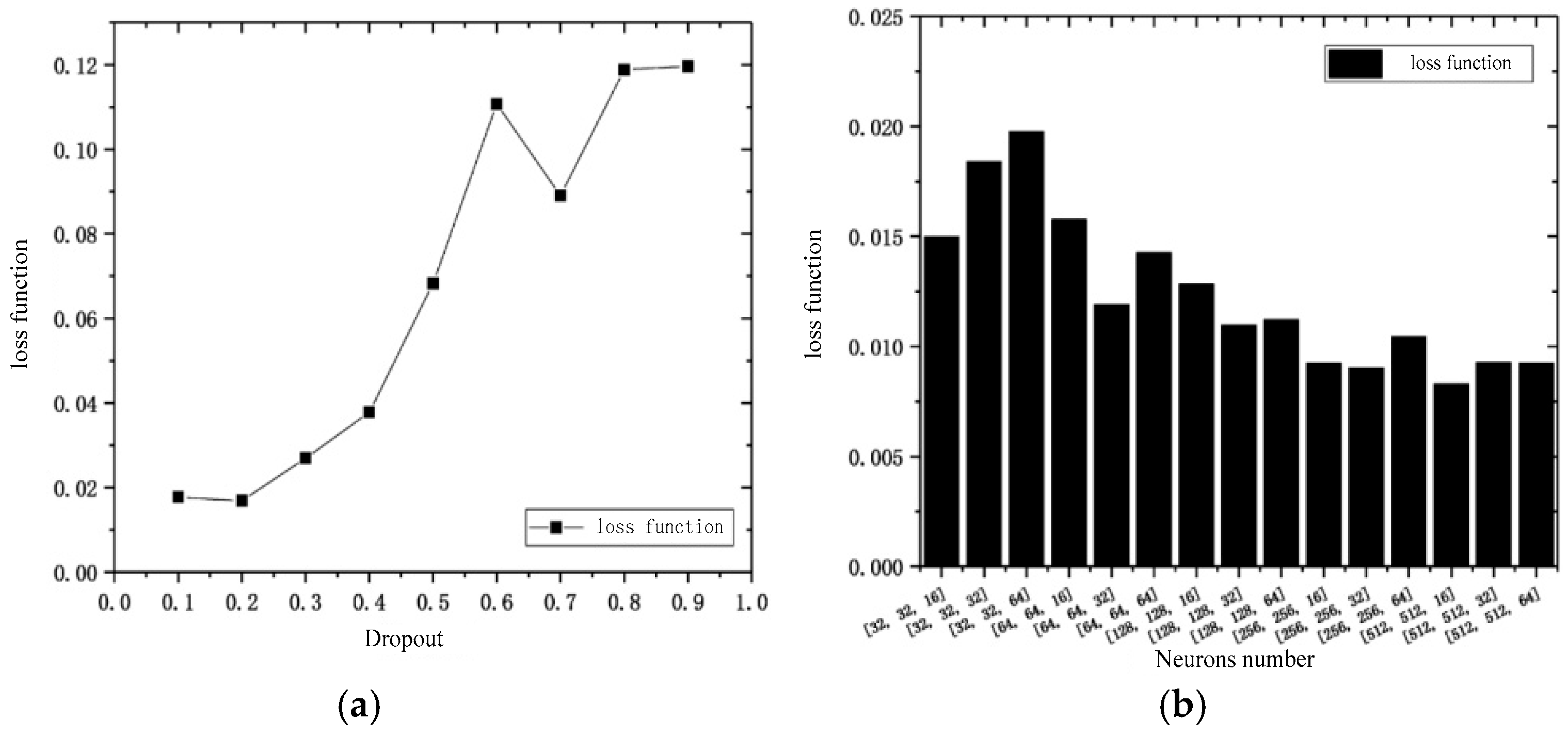
3.4.2. Model Construction

In the model, two LSTM layers are first used to obtain the time correlation information in the sample fully, and the dropout layer is added after each LSTM layer. The dropout layer is used to randomly disconnect a certain percentage of neurons in the LSTM layer to prevent overfitting in model training. Finally, two dense layers are used, and the activation function is “relu” to ensure faster training speed. Two dense layers provide more nonlinear fitting capability for the model. The model optimizer is “adam”, and the loss function is “mse” to ensure convergence. The structure of the prediction model is shown in

Table 2. Structure of prediction model.

Layer Number	Layer	Layer Number	Layer
1	LSTM layer	4	Dropout layer
2	Dropout layer	5	Dense layer
3	LSTM layer	6	Dense layer

.

The traffic data prediction diagram of the intersection entrance section based on the LSTM neural network is shown in Figure 7.

After the model structure is roughly built, the space mean speed and the vehicle steering ratio of the road entrance section are respectively sent into the model for training. Finally, different models are obtained to predict the corresponding type of traffic data. A randomly selected 70% portion of the samples is sent into the model for training, and the remaining 30% of the samples are used as test sets. In order to improve the prediction accuracy of the model, the parameters of the model need to be adjusted. Based on the structure of this model, the main adjusted parameters are the number of neurons in the LSTM layer and the dense layer and the proportion of disconnected neurons in the dropout layer. The proportion of disconnected neurons at the dropout layer increases from 0.1 to 0.9 in increments of 0.1, and the proportion at the lowest loss function value is selected as the model parameter. The selection range of the neuron numbers in the LSTM layer is [32, 64, 128, 256, 512]. The selection range of the number of neurons in the dense layer (the number of dense layer neurons in the last layer is 1) is [16, 32, 64]. The neuron number of the lowest loss function value was selected as the model parameter.

3.4.3. Model Evaluation Index

Mean absolute percentage error (MAPE) and root mean square error (RMSE) were used to evaluate the prediction effect of the model, as in (17) and (18).

$$MAPE={\displaystyle \frac{100\%}{n}}\sum _{t=1}^n\left|{\displaystyle \frac{{\widehat{x}}^t-x^t}{x^t}}\right|$$

(17)

$$RMSE=\sqrt{{\displaystyle \frac{1}{n}}\sum _{t=1}^n{\left({\widehat{x}}^t-x^t\right)}^2}$$

(18)

where $n$ is the number of test set samples, ${\widehat{x}}^t$ is the traffic data value in the predicted time period $t$, and $x^t$ is the actual traffic data value corresponding to the time period $t$.

4. Experiment and Result Analysis

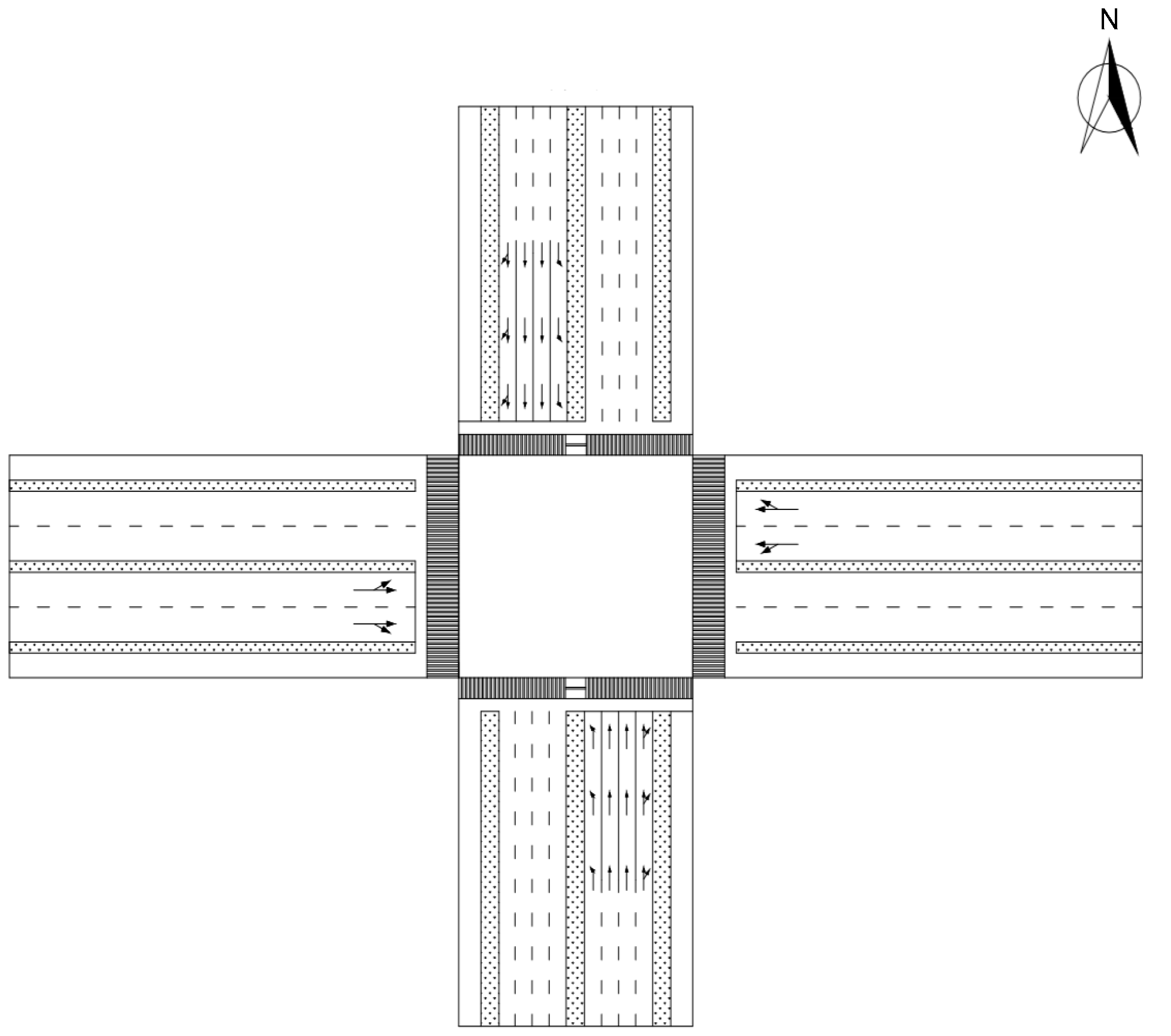
4.1. Experimental Intersection Information

An intersection in Xi’an of China is selected as an experimental case. Wi-Fi data acquisition devices are deployed at the intersection. This system is designed to verify the traffic information detection method of a single intersection based on Wi-Fi data acquisition devices.

Figure 8 shows the locations of Wi-Fi data collection devices.

Table 3. Wi-Fi data collection device information.

Device Group Number	The Coordinate of Latitude and Longitude	Distance from Intersection (m)
1	[108.953867, 4.336224]	0
2	[108.953525, 4.335852]	0
3	[108.944506, 4.336089]	831
4	[108.953489, 4.332886]	336
5	[108.960119, 4.335911]	574
6	[108.953885, 4.339578]	388

shows the information of each Wi-Fi data collection device group.

This experimental intersection is a typical cross-shaped one. The traffic volume in the north–south direction is relatively large, serving as the main arterial road, while the traffic volume in the east–west direction is relatively small, serving as the secondary arterial road. The specific channelization design of the experimental intersection is shown in Figure 9. Considering the traffic demand of the main roads, both the south and north entrances are designed with four lanes, namely, one left-turn-only lane, two straight lanes, and one lane for both straight and right turns. The traffic flow at the east and west entrances is relatively small. Both entrances are designed with two lanes. The first one is a shared lane for straight-going vehicles turning left and right, while the second one is a shared lane for straight-going vehicles turning right only.

4.2. Traffic Information Detection

By applying the aforementioned method, real-time preprocessing of Wi-Fi data is carried out, and the detection of road targets passing through the intersection is achieved based on MAC address matching. The road target data set from 9:00 to 21:00 on a working day is taken as an example to distinguish road target travel modes. The data can be obtained using a combination of field surveys and Baidu Map data. The data set contains 7107 samples.

First, the elbow method is used to determine the optimal clustering K-value. The SSE value of the data set has the largest decline when the value is 2; therefore, the clustering value of this data set is set to 2, as shown in Figure 10a. At this point, if direct clustering is adopted, the data set is divided into two clusters. Among them, the number of samples in the cluster of category 0 is 4388, and the mean speed of the import section of the center point is 30.656 km/h, while that of the export section is 26.839 km/h, with a speed difference of 19.023 km/h. The number of samples in the cluster of category 1 is 2540, and the mean speed of the import section of the center point is 14.605 km/h, while that of the export section is 15.178 km/h, with a speed difference of 7.221 km/h. It can be seen that the values of each feature of Category 0 and Category 1 are overall higher, which does not match the travel speed of low-speed targets in reality.

Subsequently, a clustering profile analysis was performed. The road target data set was adjusted, and the vehicle speed threshold was successively selected within the interval [10,25] for clustering, as shown in Figure 10b. The average silhouette coefficient has the largest value when the vehicle speed threshold is 13 km/h, so the vehicle speed threshold for this data set is selected as 13 km/h. After adjusting the road target data set according to the selected motor vehicle speed threshold, the sample number is 897. K-means clustering is carried out. Among them, the number of samples in the cluster of category 0 is 495, and the speed of the central point of the import section of the cluster is 9.324 km/h, the speed of the export section is 9.367 km/h, and the speed difference between the import and export sections is 3.833 km/h. The number of samples in the cluster of category 1 is 402, and the speed of the central point of the import section is 5.254 km/h, the speed of the export section is 4.981 km/h, and the speed difference is 1.681 km/h. The travel speed of the samples in Category 0 is motor vehicles, and the travel speed of the samples in Category 1 is walking and non-motorized vehicle travel. The number of samples between the two clusters is more balanced, and the speed characteristics of the clustering center of the low-speed road target are significantly reduced, which is more consistent with the actual situation. The method of optimizing the clustering profile analysis is relatively effective.

Finally, spatial-temporal correlation analysis is used to divide the travel modes of the motor vehicle travel samples into private car and bus travel. In the above 6705 samples of motor vehicle travel, the number of bus travel was 1215, and the number of buses was 232. It can be seen that the road targets with bus as the primary mode of transportation account for a relatively large proportion. Therefore, it is necessary to distinguish the travel modes of road targets.

After the road target travel mode is distinguished, the road target is visualized. Finally, the space mean speed and time series of vehicle steering ratio of each road entrance section and exit section of the intersection are obtained by using the sliding time window method. The statistical period is 15 min. Figure 11, Figure 12 and Figure 13 show the space mean speed and vehicle steering ratio information obtained from the collected Wi-Fi data during 9:00–21:00 on a working day at the intersection. In order to show more details of the traffic information changes, the step length of the time sliding window is set to 1 min.

From the above traffic information, it can be clearly seen that there is an obvious evening peak at the intersection between 18:00 and 19:00. The space mean speed of the exit and entrance sections in each direction decreased significantly. There is no obvious rule in the proportion of left-turning vehicles in the entrance sections in each direction, and the fluctuation is more drastic.

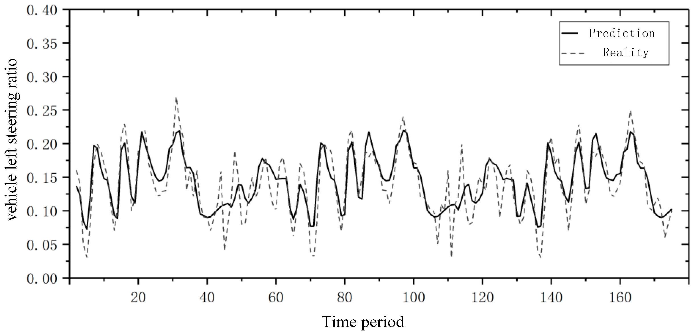
4.3. Predictive Model Training and Verification

After the space mean speed and proportional time series data at intersections are preprocessed, 726 samples are obtained for the training model. In the time series reconstruction, the value of n is 14. That is, the space mean speed and vehicle steering ratio at the next moment of the intersection entrance section are predicted by the data of the previous 15 time periods from itself and the three downstream entrance sections.

The Keras framework is used to construct and adjust the model structure. After the model structure is roughly built, 70% of the samples are randomly selected into the model for training, and the remaining 30% of samples are used as the test sets. In order to improve the prediction accuracy of the model, its parameters need to be adjusted. For example, the space mean speed prediction model of the south road entrance section shows the adjustment process of the neuron number and the dropout ratio in Figure 14. With the same number of iterations, the MSE of the test set sample is the lowest when the proportion of disconnected neurons in the dropout layer is 0.2. When the number of neurons in each layer is (256,256,32), the MSE of the test set sample is sufficiently low, and the number of neurons is moderate. Subsequently, the model parameters are determined.

After the parameters are adjusted, the model is trained using the set, and the test set is fed into the model for prediction. Taking the traffic data of the south road entrance as an example, Figure 15 and Figure 16 show the single-step prediction results of the test set model. The model can predict the traffic data of space mean speed and vehicle steering ratio well. The predicted value is close to the real value and can better follow the real data change trend.

Table 4. Statistical table of error evaluation of vehicle left steering ratio prediction model.

Error	North	South	East	West
RMSE (Textual reconstruction method)	0.01713	0.01642	0.02594	0.02041
MAPE (Textual reconstruction method)	12.8634	10.07899	10.1695	11.9669
RMSE	0.017605	0.021753	0.02827	0.02743
MAPE	13.69658	13.15832	10.5006	12.2864

and

Table 5. Statistical table of error evaluation of the space mean speed prediction model of the road entrance section.

Error	North	South	East	West
RMSE (Textual reconstruction method)	0.64729	0.93593	0.99953	0.958572
MAPE (Textual reconstruction method)	2.79431	3.26728	3.41611	3.6238
RMSE	0.66443	1.067952	1.25264	0.72434
MAPE	3.10929	3.50150	4.48097	2.93503

show the error evaluation of the space mean speed and vehicle left steering ratio prediction models of the entrance sections in each direction. The prediction error evaluation was low for different data sets. Additionally, the error evaluation of the model-trained prediction results by using the reconstructed sample, only considering the data of the entrance road section, and the reconstructed sample in this study is compared. The MAPE and RMSE of the model prediction results for the reconstructed samples in this study were generally smaller. The experimental results show that the model has a better prediction effect, and the validity of the proposed reconstruction method is demonstrated.

5. Conclusions

This study proposes a traffic information detection method at a single intersection based on Wi-Fi data.

(1)

The hardware architecture of Wi-Fi data acquisition equipment is determined to realize the collection of Wi-Fi data at a single intersection.

(2)

This study combined MAC address matching, k-means clustering, sliding time window, and other algorithms to process and analyze the Wi-Fi data of a single intersection and realize the detection of the spatial average speed of the entrance and exit sections of a single intersection and the vehicle turning proportion information of the entrance section.

(3)

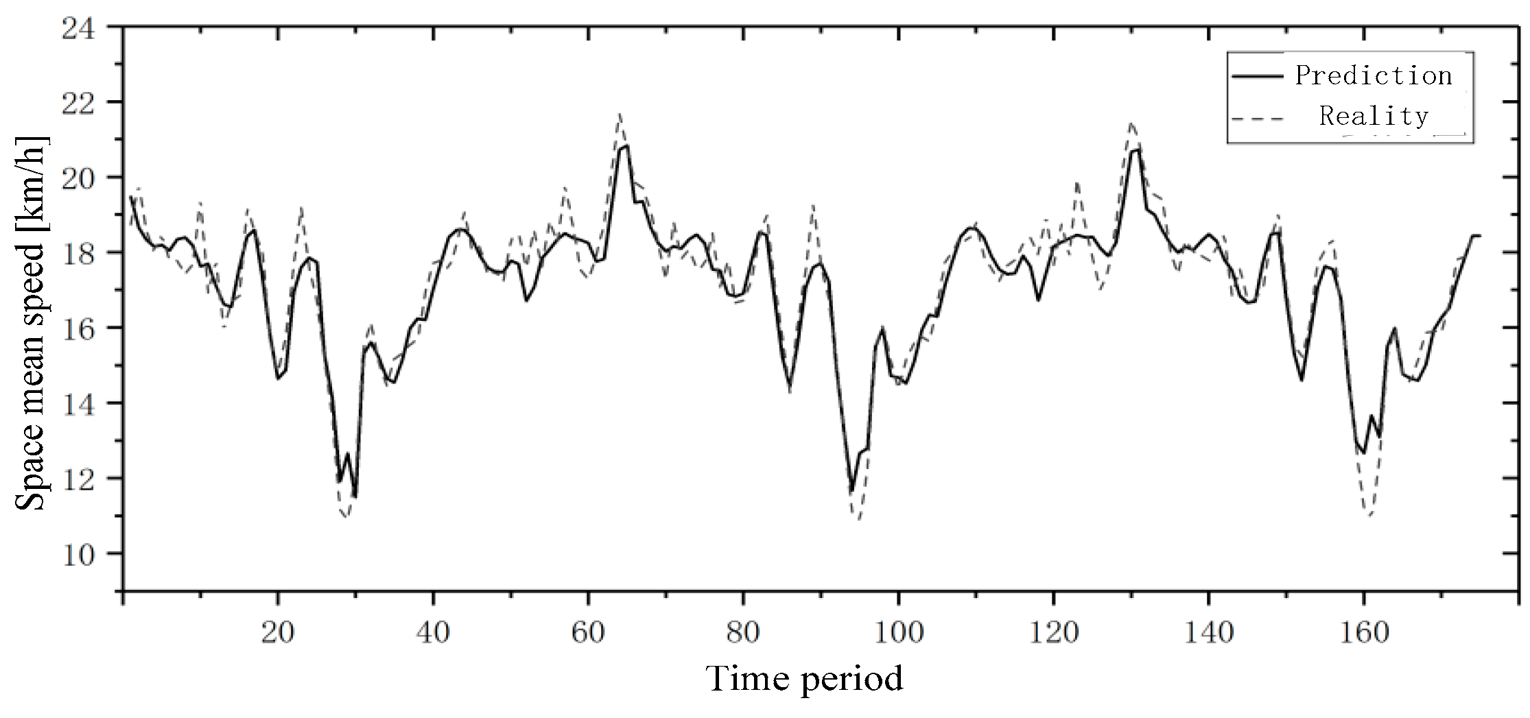
The function of a single-point intersection traffic information detection scheme based on Wi-Fi data acquisition equipment is expanded. The traffic data prediction model of the intersection inlet section based on the LSTM neural network is constructed, and the training of the prediction model is completed in the Keras framework so as to predict the spatial average speed and vehicle turning ratio of the intersection inlet section.

This study shows the error evaluation of the spatial average speed and the left-turn ratio prediction model of the inlet road section in each direction under the case verification. For different data sets, the prediction error evaluation is low. The error evaluation of the prediction results of the model trained by using the reconstructed samples only considers the data of the inlet road section, and the reconstructed samples in this paper are compared. The MAPE and RMSE of the model prediction results of the reconstructed samples in this paper are generally smaller, indicating that the prediction effect is better and that the proposed method is effective.

The data collected in this study were obtained on sunny working days, which has certain limitations. Further research will be conducted to expand to the following aspects:

(1)

Taking into account the influence of the surrounding environment, in our subsequent research, we will adopt complementary technologies to expand the research scope to multiple intersections and also consider the impact of complex environments (different days, seasons, weather conditions, etc.) on the collection of Wi-Fi signals.

(2)

Multi-step prediction and sliding-window forecasting approaches are the research directions for us in the future.

References

- Danesh, A.; Ma, W.; Wang, L. Identifying the adaptability of different control types based on delay and capacity for isolated intersection. Transport. Res. Rec. 2023, 2677, 33–45. [Google Scholar] [CrossRef]
- Wu, J.J. Congestion control method for urban traffic intersections by integrating Internet of Things and traffic flow data. Comput. Inform. Mech. Syst. 2022, 5, 86–91. [Google Scholar]
- Zhang, Y.; Shang, K.; Cui, Z.; Zhang, Z.; Zhang, F. Research on traffic flow prediction at intersections based on DT-TCN-attention. Sensors 2023, 23, 6683. [Google Scholar] [CrossRef] [PubMed]
- Xu, M.; Qiu, T.Z.; Fang, J.; He, H.; Chen, H. Signal-control refined dynamic traffic graph model for movement-based arterial network traffic volume prediction. Exp. Syst. Appl. 2023, 228, 120393. [Google Scholar] [CrossRef]
- Azimjonov, J.; Özmen, A.; Varan, M. A vision-based real-time traffic flow monitoring system for road intersections. Multimed. Tools Appl. 2023, 82, 25155–25174. [Google Scholar] [CrossRef]
- Yue, G.; Li, Z.; Tao, Y.; Jin, T. Low-illumination traffic object detection using the saliency region of infrared image masking on infrared-visible fusion image. J. Electron. Imaging. 2022, 31, 3. [Google Scholar] [CrossRef]
- Liu, C.C.; Liang, Y.P.; Zhang, X.L. The analysis and advanced development of traffic flow information acquisition technology in ITS. Appl. Mech. Mater. 2014, 536, 828–832. [Google Scholar] [CrossRef]
- Guo, C.; Li, D.; Chen, X. Unequal Interval Dynamic Traffic Flow Prediction with Singular Point Detection. Appl. Sci. 2023, 13, 8979. [Google Scholar] [CrossRef]
- Liu, H.; Teng, K.; Rai, L.; Zhang, Y.; Wang, S. A two-step abnormal data analysis and processing method for millimetre-wave radar in traffic flow detection applications. IET Intell. Transp. Syst. 2021, 15, 671–682. [Google Scholar] [CrossRef]
- Huang, S.; Sun, D.; Zhao, M.; Chen, J.; Chen, R. Short-term traffic flow prediction approach incorporating vehicle functions from RFID-ELP data for urban road sections. IET Intell. Transp. Syst. 2023, 17, 144–164. [Google Scholar] [CrossRef]
- Bhargava, K.; Wah Choy, K.; Jennings, P.A.; Higgins, M.D. Novel mathematical model to determine geo-referenced locations for C-ITS communications to generate dynamic vehicular gaps. IET Intell. Transp. Syst. 2021, 14, 2010–2020. [Google Scholar] [CrossRef]
- Iqbal, R.; Yukimatsu, K. Intelligent transportation systems using short range wireless technologies. J. Transport. Technol. 2011, 1, 132–137. [Google Scholar] [CrossRef]
- Radu, V.; Kriara, L.; Marina, M.K. Pazl: A mobile crowdsensing based indoor WiFi monitoring system. In Proceedings of the 9th International Conference on Network and Service Management (CNSM 2013), Zurich, Switzerland, 14–18 October 2013. [Google Scholar]
- Gao, S.; Liu, Y.; Wang, Y.; Ma, X. Discovering spatial interaction communities from mobile phone data. Trans. Gis. 2013, 17, 463–481. [Google Scholar] [CrossRef]
- Prentow, T.S.; Ruiz-Ruiz, A.J.; Blunck, H.; Stisen, A.; Kjærgaard, M.B. Spatio-temporal facility utilization analysis from exhaustive wifi monitoring. Pervasive Mob. Comput. 2015, 16, 305–316. [Google Scholar] [CrossRef]
- Cunche, M. I know your MAC address: Targeted tracking of individual using Wi-Fi. J. Comput. Virol. Hack. Tech. 2014, 10, 219–227. [Google Scholar] [CrossRef]
- Hidayat, A.; Terabe, S.; Yaginuma, H. Determine non-passenger data from WiFi scanner data (MAC address), a case study: Romango bus, Obuse, Nagano prefecture, Japan. Int. Rev. Spat. Plan. Sustain. Dev. 2018, 6, 154–167. [Google Scholar] [CrossRef]
- Xu, Z.; Zhao, J.; Lin, C. Pedestrain monitoring system using Wi-Fi technology and RSSI based localization. Int. J. Wirel. Mobile Netw. 2013, 5, 17–34. [Google Scholar] [CrossRef]
- Zhao, F.; Shi, W.; Gan, Y.; Peng, Z.; Luo, X. A localization and tracking scheme for target gangs based on big data of Wi-Fi locations. Cluster Comput. 2019, 22, 1679–1690. [Google Scholar] [CrossRef]
- Huang, Z.; Xu, L.; Lin, Y. Multi-stage pedestrian positioning using filtered WiFi scanner data in an urban road environment. Sensors 2020, 20, 3259. [Google Scholar] [CrossRef]
- Zhang, S.; Ni, B. Science and education integration mode python-c experimental teaching research design of WiFi line avoidance vehicle. In Communications, Signal Processing, and Systems; Springer: Singapore, 2023. [Google Scholar]
- Kochańska, J.; Burduk, A.; Markowski, M.; Klusek, A.; Wojciechowska, M. Improvement of factory transport efficiency with use of WiFi-based technique for monitoring industrial vehicles. Sustainability 2023, 15, 1113. [Google Scholar] [CrossRef]
- Chen, H.C.; Lin, R.S.; Huang, C.J.; Tian, L.; Su, X.; Yu, H. Bluetooth-controlled parking system based on WiFi positioning technology. Sens. Mater. 2022, 34, 1179–1189. [Google Scholar] [CrossRef]
- Mazokha, S.; Bao, F.; Zhai, J.; Hallstrom, J.O. MobIntel: Sensing and analytics infrastructure for urban mobility intelligence. Pervasive Mob. Comput. 2021, 77, 101475. [Google Scholar] [CrossRef]
- Oransirikul, T.; Nishide, R.; Piumarta, I.; Takada, H. Measuring bus passenger load by monitoring Wi-Fi transmissions from mobile devices. Procedia Technol. 2014, 18, 120–125. [Google Scholar] [CrossRef]
- Hidayat, A.; Terabe, S.; Yaginuma, H. WiFi scanner technologies for obtaining travel data about circulator bus passengers: Case study in Obuse, Nagano prefecture, Japan. Transport. Res. Rec. 2018, 2672, 45–54. [Google Scholar] [CrossRef]
- Hidayat, A.; Terabe, S.; Yaginuma, H. Estimating bus passenger volume based on a Wi-Fi scanner survey. Transp. Res. Interdiscip. Perspect. 2020, 6, 100142. [Google Scholar] [CrossRef]
- Ahmed, H.; El-Darieby, M.; Morgan, Y.; Abdulhai, B. A wireless mesh network-based platform for ITS. In Proceedings of the VTC Spring 2008—IEEE Vehicular Technology Conference, Marina Bay, Singapore, 11–14 May 2008. [Google Scholar]
- Vieira, T.; Almeida, P.; Meireles, M.; Ribeiro, R. Public transport occupancy estimation using WLAN probing and mathematical modeling. Transport. Res. Procedia. 2020, 48, 3299–3309. [Google Scholar] [CrossRef]
- Won, M.; Zhang, S.; Son, S.H. WiTraffic: Low-Cost and Non-Intrusive Traffic Monitoring System Using WiFi. In Proceedings of the 2017 26th International Conference on Computer Communication and Networks (ICCCN), Vancouver, BC, Canada, 31 July–3 August 2017. [Google Scholar]
- Oransirikul, T.; Piumarta, I.; Takada, H. Classifying passenger and non-passenger signals in public transportation by analysing mobile device Wi-Fi activity. J. Inf. Process. 2019, 27, 25–32. [Google Scholar] [CrossRef]
- Leng, B.; Huang, L.; Qiao, C.; Xu, H. Urban Traffic Condition Estimation: Let WiFi Do It. In Proceedings of the 2016 13th Annual IEEE International Conference on Sensing, Communication, and Networking (SECON), London, UK, 27–30 June 2016. [Google Scholar]
- Marakkalage, S.H.; Yuen, C.; Yow, W.Q.; Chong, K.H. WiFi fingerprint clustering for urban mobility analysis. IEEE Access. 2021, 9, 69527–69538. [Google Scholar] [CrossRef]
- Cai, X.; Tan, J.; Lu, Z. Multi mobile robot positioning technology and path planning design based on WiFi Positioning. In Proceedings of the 2022 International Conference on Computer, Electronic and Materials Engineering (ICCEME 2022), Taiyuan, China, 18–19 June 2022. [Google Scholar]
- Alam, S.S.; Al-Qurishi, M.; Souissi, R. Estimating indoor crowd density and movement behavior using WiFi sensing. Front. Internet Things 2022, 1. [Google Scholar] [CrossRef]
- Asim, M.A.; Kattan, L.; Wirasinghe, S.C. Smartphone: A source for transit service planning and management using WIFI sensor data. In Proceedings of the Canadian Society of Civil Engineering Annual Conference 2021, Whistler, BC, Canada, 26–29 May 2021. [Google Scholar]
- Hidayat, A.; Terabe, S.; Yaginuma, H. Mapping of MAC Address with Moving WiFi Scanner. Int. J. Artif. Intell. Res. 2017, 1, 34–40. [Google Scholar] [CrossRef]
- Rao, W.; Xia, J.; Lyu, W.; Lu, Z. Interval data-based k-means clustering method for traffic state identification at urban intersections. IET Intell. Transp. Syst. 2019, 13, 1106–1115. [Google Scholar] [CrossRef]