Abstract
This paper presents a novel approach for screening women in their first trimester of pregnancy to identify those at high risk of having a child with Down syndrome (DS), using machine learning algorithms. Various machine learning models, including statistical, linear, and ensemble models, were trained using a pseudo-anonymized dataset of 90,532 screening patients. This dataset, containing less than 1% positive cases, was obtained from Cruces University Hospital, a public health hospital (Osakidetza) in Baracaldo, Basque Country, Spain. The models incorporate a set of input variables, including demographic variables such as maternal age, weight, ethnicity, smoking status, and diabetes status, as well as laboratory variables like nuchal translucency (NT), pregnancy-associated plasma protein-A (PAPP-A), and beta-human chorionic gonadotropin hormone (B-HCG) levels. The trained classification algorithms achieved ROC-AUC values between 0.970 and 0.982, with sensitivity and specificity of 0.94. The results indicate that machine learning techniques can effectively predict Down syndrome risk in first-trimester screening programs.
1. Introduction
Down syndrome is a genetic condition in which approximately 95% of individuals with this syndrome have an extra full or partial copy of chromosome 21. This results in chromosome 21 being present in three copies, instead of the usual two, in each cell [1].
A research study conducted from 2010 to 2014 estimated the prevalence of trisomy 21 (T21) to be approximately 6000 births per year [2]. While this represents about 1 in 700 births, Loane et al. suggest that this trend may be increasing in Europe due to the rising average maternal age, a known risk factor for the condition [3].
Individuals diagnosed with Down syndrome commonly exhibit a range of associated conditions, including intellectual and developmental disabilities, as well as neurological manifestations such as congenital cardiac problems and gastrointestinal abnormalities [1]. They may also display distinctive facial features and experience other abnormalities such as hematologic disorders [4]. However, it is important to acknowledge that the severity and extent of these conditions can vary significantly among individuals, as noted by the National Down Syndrome Society (NDSS). Thanks to advances in medical research, the life expectancy of individuals with T21 is now longer, with a survival age of 60 years among 80% of adults with the condition.
Despite the progress made and the increasing integration of individuals with T21 into society, it remains crucial for parents to have accurate information about the likelihood of their unborn child having this condition during the early stages of pregnancy. This is particularly important given that many countries offer parents the option to terminate a pregnancy based on medical criteria, informed by technical methods designed to predict positive T21 outcomes. Most public health systems have established screening programs to identify pregnant women at high risk of carrying a fetus with trisomy 21 [5,6,7]. These programs typically calculate the risk of T21 based on four markers: nuchal translucency, maternal age, and the hormones PAPP-A and B-HCG [8,9,10]. Standard statistical modeling techniques are employed in these calculations [11]. However, these screening methods are not infallible and can produce false-positive results, indicating a high risk when the fetus does not have Down syndrome. Traditional screening detects 89% of fetuses with T21, with a false positive rate of 5%. Furthermore, maternal factors such as advanced maternal age and maternal weight can influence the accuracy of these assessments, potentially leading to inaccurate risk predictions [12,13,14]. These inaccuracies can cause unnecessary anxiety for expectant parents and may lead to the use of invasive diagnostic procedures like amniocentesis or chorionic villus sampling (CVS), both of which carry a small but significant risk of gestational loss (0.1–1%) [15]. Amniocentesis involves extracting amniotic fluid through a needle inserted into the abdomen, while CVS retrieves placental tissue through the cervix or abdomen. Given the inherent risks of these procedures, screening programs should strive for the highest possible detection rate with the lowest possible false-positive rate. Consequently, there is a clear need for improved screening methodologies that offer higher detection rates and lower false-positive rates, thereby reducing reliance on invasive diagnostic procedures.
In recent years, machine learning techniques have been increasingly applied to this use case to improve prediction accuracy and prenatal screening [16,17]. Machine learning algorithms can analyze complex datasets and identify patterns that may not be apparent using traditional statistical methods. These algorithms can integrate various data sources, including maternal serum markers, ultrasound measurements, and even cell-free DNA information, to provide more accurate risk assessments. Several studies have demonstrated the potential of machine learning in prenatal screening. For instance, researchers have explored the use of support vector machines (SVMs), random forests, and neural networks to predict the risk of Down syndrome and other chromosomal abnormalities. For example, Koivu et al. achieved an area under the ROC curve of 0.96 and a detection rate of 78%, with a 1% false positive rate in the first trimester using a cohort of 1850 individuals [18]. He et al. published a study with 58,972 screening data that achieved a 0.89 ROC-AUC, although the prediction in that work was for the second trimester [16]. The work of Jamshidnezhad et al. is also relevant; they reported a specificity of 99.72%, a sensitivity of 90.91%, and a mean square error of 0.61%, but these figures are based on the average of 10 experiments with a limited population of only 381 pregnant women [19]. Furthermore, machine learning can be used to personalize risk assessment by incorporating individual maternal characteristics, potentially leading to more tailored and accurate screening results. While the application of machine learning in prenatal screening is still an evolving field, the initial results are promising and suggest that these techniques have the potential to significantly improve the accuracy and safety of Down syndrome screening.
This paper presents the design, implementation, and validation of a training pipeline for various machine learning models to predict T21 risk during the first trimester of pregnancy. A key aspect of this approach is the optimization of these models through an automated search for hyperparameters, aiming to maximize detection rates while minimizing false positive occurrences. This process is carried out using optimization algorithms to identify the optimal combinations of hyperparameters. The study utilizes a cohort of 110,238 pregnant women, with less than 1% positive cases, from Cruces University Hospital, a public health hospital (Osakidetza) in Baracaldo, Basque Country, Spain.
The following sections of this paper detail the key components of our study, beginning with Section 2 (Methodology), which introduces the background of the problem, and Section 2.1, which describes the data extraction process in detail. Section 2.2 explains the data preparation steps, and Section 2.3 details the training pipeline. Section 3 (Results) presents the main metrics for the trained classifiers. Section 4 (Discussion) explains and evaluates the results. Section 5 (Conclusions) concludes this paper.
2. Methodology
The Basque Country currently has a screening program for Down syndrome. This program calculates the risk based on nuchal translucency, maternal age, and two hormones (PAPP-A and B-HCG) between 11 + 0 and 13 + 6 weeks of pregnancy. Clinical data and marker values are recorded in an application that performs the calculations according to the prediction model published by the Nicolaides group [20]. In addition to recording screening calculations, the program also records all invasive tests, their results, and all perinatal outcomes. With a false-positive rate of 5%, this method achieves a trisomy 21 detection rate of approximately 90%, surpassing the 30% detection rate achieved by maternal age alone. While this represents a significant improvement over previous clinical practice, there is still room for improvement in the model. Key indicators of model performance include accuracy, a high detection rate, and a high positive predictive value. Enhancing these parameters without compromising others would lead to a better screening model.
2.1. Data Extraction
This work uses a pseudo-anonymized dataset from Cruces University Hospital, located in Baracaldo, Basque Country, Spain. The dataset comprises patients from the Bilbao area. Originally, it contained 102 features related to 133,708 pregnant women, with births spanning from 2009 to 2019.
It is crucial to emphasize that our research team received a pseudo-anonymized version of the dataset. The original data extraction and pseudonymization were conducted by the Cruces University Hospital staff, and we were provided with data that lacked direct personal identifiers (e.g., patient names and identification numbers). The specific methods employed by the hospital to pseudonymize the data are governed by their internal protocols and ethical guidelines, which adhere to relevant data protection regulations.
The first step in our data extraction process was to create a detailed data dictionary in collaboration with the medical team to ensure a comprehensive understanding of the features. This process, led by the clinical team, enabled the exclusion of features that did not provide relevant information (e.g., constants, IDs, etc.) and features related to stages beyond the first trimester. Multiple-pregnancy cases were also removed from the dataset, as they differ clinically from single-pregnancy cases. After this initial pre-processing stage, the dataset was reduced to 9 out of the original 102 features and 109,386 samples.
2.2. Data Preparation
Once the data were deemed morphologically correct from a clinical perspective and all information was limited to the first trimester, the next step involved preparing it for the training phase. This data preparation stage consisted of three steps, detailed in the following subsections. Section 2.2.1 describes the exploratory data analysis (EDA) conducted to extract the dataset’s main characteristics. This EDA, a crucial component of any machine learning workflow, guided the subsequent steps of handling missing values (Section 2.2.2) and removing outliers (Section 2.2.3). The findings from the EDA also informed decisions made during the design of the training workflow, as described in Section 2.3.
2.2.1. Exploratory Data Analysis
The primary objective of this stage was to gain a deeper understanding of the underlying data to clarify feature importance and select the features with the greatest impact on the training workflow. To achieve this, the distribution of the features was examined, combining clinical knowledge with insights derived from the data. The features “ethnicity”, “diabetes”, “smoker”, and “familiar antecedents” were excluded from the training phase due to the low proportion of samples with diverse ethnicities and the small percentage of pregnant women with diabetes or a family history of T21 or T18–T13. Specifically, this exclusion was based on the principle that features with very few representative samples can introduce bias and instability into machine learning models, reducing their ability to generalize well. Figure 1 illustrates the Pearson correlation between features, revealing a correlation between PAPP-A, NT, B-HCG, age, and the trisomy 21 diagnosis. Pearson correlation, a standard measure of linear association, was used here to quantify the extent to which these variables change together. The correlation coefficient ranges from −1 to +1, where values close to −1 or +1 indicate a strong linear relationship and values near 0 indicate a weak linear relationship. It is important to note that while some correlations are observed, many of them are quite small, suggesting limited linear dependencies between those variables. Low PAPP-A values correlate with positive T21 cases (meaning PAPP-A tends to decrease as the likelihood of T21 increases), while high B-HCG and NT values also correlate with positive cases (meaning B-HCG and NT tend to increase with the likelihood of T21). These relationships are further shown in Figure 2. Following this step, only four features were selected for the training phase—age, PAPP-A, B-HCG, and NT—in addition to the outcome variable itself.
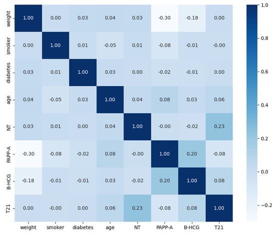
Figure 1.
Pearson correlation matrix, illustrating the pairwise linear relationships between the variables used in this study. The color intensity and numerical values indicate the strength and direction of the correlation.
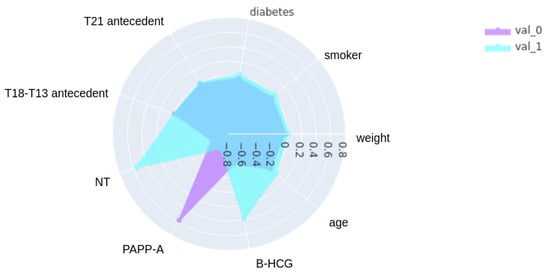
Figure 2.
Radar plot showing the correlation of variables with trisomy 21 status. This radar plot visualizes the correlation between each variable and the trisomy 21 (T21) outcome, comparing correlation patterns for negative cases (Negative Cases) and positive cases (Positive Cases). The variables are arranged in a clockwise direction for visual clarity. Larger areas indicate stronger correlations.
The next objective of the EDA process was to guide the remaining data pre-processing tasks described in the following sections.
2.2.2. Missing Values
When handling missing values in a dataset, two main approaches are possible: discarding samples or imputing the missing values. The current dataset contains 18,732 samples with at least one missing value. Although this is a considerable number, only 10 of these samples are positive cases. Given the relatively large number of negative samples and the small proportion of positive samples, the decision was made to remove the samples with missing values. This choice was based on the assumption that it would have an insignificant impact on training performance. This decision is also supported by the fact that various data balancing techniques will be employed during model training, as detailed in subsequent sections. After removing rows with missing values, the dataset comprised 90,654 cases.
2.2.3. Outlier Removal
Another important consideration before training a data model is the presence of outliers in the dataset. Data collection invariably involves a risk of errors (e.g., human transcription errors) that can affect or bias classification performance. Outliers can also occur due to anomalies in some samples, such as a person being overweight or having unusually high levels of a certain protein. Therefore, it is essential to detect and remove outliers from the dataset before training.
The following features from the original dataset were examined for outliers: weight, age, PAPP-A, B-HCG, and NT. Grubbs’ test [21], also known as the maximum normed residual test, was used to detect outliers in these features, with a significance level of p < 0.01. Grubbs’ test is suitable for univariate datasets that approximately follow a normal distribution and is designed to detect single outliers. This analysis identified 53 outliers for weight, 1 for age, 354 for PAPP-A, 232 for B-HCG, and 231 for NT. These samples were sent to clinicians for confirmation of their erroneous nature and safe removal from the dataset. After these data preparation steps, the final dataset consisted of 90,532 cases, as described in Table 1.

Table 1.
Dataset after removing missing values and outliers. Mean ± standard deviation is shown for numerical variables, and counts with percentages are shown for categorical variables.
2.3. Training Workflow
After the data preparation stage, the data were ready for the training workflow, illustrated in Figure 3, which consists of the following building blocks: splitting (Section 2.3.1), pipeline creation (Section 2.3.2), training (Section 2.3.3), and validation (Section 2.3.4).
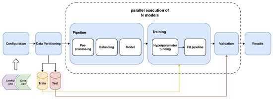
Figure 3.
Machine learning model training workflow. This figure depicts the complete process for training and validating the machine learning models. The workflow begins with the input of the configuration file and the dataset. The data are then split into training and test sets. The training set undergoes a series of pipeline steps: pre-processing (including scaling and encoding), balancing (using SMOTE and undersampling), and model fitting. Hyperparameter optimization is performed to tune the model parameters. The trained model’s performance is then evaluated using the held-out test set, and the final performance metrics are reported.
2.3.1. Splitting
The primary purpose of the splitting step is to prevent overfitting, a phenomenon where a model performs well on the data it has already seen but poorly generalizes to unseen data. In this process, the dataset is divided into two subsets: a “training data” subset, comprising 80% of the original samples, and a “test data” subset, containing the remaining 20% of the original dataset. The test data are put aside to validate the resulting models with unseen data at the end of the training phase. The splitting process involves (1) shuffling all samples to eliminate any potential bias caused by the original order and (2) maintaining the original proportion of the outcome variable in both subsets using stratified splits.
2.3.2. Pipeline Building
Prior to the training stage, a pipeline of transformers and a final estimator is constructed. This pipeline is used in both the training and validation steps, ensuring that all transformations are consistently applied to the training, validation, and prediction data. As shown in Figure 3, the pipeline comprises three steps: pre-processing, balancing, and modeling. The first two transformation steps are applied sequentially, followed by the execution of a final estimator, enabling cross-validation of the assembled steps.
- Pre-processing: This pipeline step distinguishes between categorical and numerical columns. Numerical columns are standardized by scaling them to have a mean of 0 and a standard deviation of 1. Categorical columns, on the other hand, are encoded using the One-Hot Encoding technique. This technique creates new categorical columns for each unique value and assigns a binary value of 1 or 0 based on the presence or absence of the corresponding value. Due to the substantial imbalance in the input features, the encoding method is fitted using the complete dataset before the data are partitioned into train/test sets and subsequent k-folds. This ensures that no trained partition lacks a value that exists in a new sample, preventing misclassification.
- Balancing: As mentioned earlier, the dataset is highly unbalanced (99.41% negative samples). Classification models typically perform poorly on such datasets because they tend to over-predict the most prevalent class. To address this issue, balancing techniques are applied within the pipeline. SMOTE (Synthetic Minority Oversampling Technique) [22] is used to increase the number of positive samples, while random under-sampling is used to balance the dataset. To achieve a balanced sample, SMOTE is systematically applied to each training set until the positive samples represent 5% of the total, followed by a random reduction in negative samples. In the model training phase using the designated training partition, the partition contains 72,424 samples, with 72,000 negative and 424 positive samples. In contrast, the final test dataset contains 18,107 samples, including 106 positive samples. During the balancing process within the training partition, SMOTE augments the positive samples until they reach 3621. Subsequently, the dataset is balanced by randomly selecting an equal number of negative samples. This approach ensures that the models are trained with balanced datasets; however, the test data remain unbalanced to avoid sample loss.
- Model: The final step in the pipeline is the insertion of the classification model, which is used for training or predicting new samples after the pipeline is fitted.
2.3.3. Model Training
Once the pipeline is constructed, the model is ready for training. K-fold cross-validation, a robust statistical technique, is employed to evaluate the performance of machine learning models and to assess how well they are expected to generalize to unseen data. In this method, the training data are partitioned into k equally sized subsets or folds. The model is trained k times, each time using k-1 of the folds as the training set and the remaining fold as a validation set. This process provides k different estimates of the model’s performance on independent data, which are then averaged to obtain a more reliable overall evaluation. The pipeline ensures that data preparation before model fitting is performed exclusively on the training data within each fold, preventing data leakage and optimistic model skill estimation. In this study, k is set to 10, and 10-fold cross-validation is conducted over five repetitions to determine the hyperparameters, providing a more robust approach and mitigating the effects of randomness in the algorithms and data partitions.
Each learning model has several hyperparameters that must be defined before training, such as the regularization term or the maximum depth of the trees. Some hyperparameters, like the regularization term, can only take one set of values, while others can take values within a range of real numbers. This creates a combinatorial problem where the number of possible combinations grows exponentially with the number of hyperparameters and the range of values for each hyperparameter. Consequently, finding an efficient solution in terms of time is an NP-complete problem. To address this, metaheuristic optimization techniques, known as hyperparameter tuning or hyperparameter optimization (HPO), are used to automate the search for hyperparameters in an efficient and intelligent manner. In this study, evolutionary algorithms (EAs) are employed for hyperparameter tuning. EAs are a class of optimization algorithms inspired by the process of biological evolution. They work with a population of candidate solutions, where each solution represents a specific combination of hyperparameters. This “population” evolves over generations through processes analogous to natural selection and genetic inheritance. The hyperparameter space serves as the initial population, and each individual in the population represents a set of hyperparameters for the machine learning model. The performance of individuals is evaluated using a performance metric, or heuristic, derived from the train/validation scores to minimize the risk of overfitting. This metric acts as a “fitness function”, guiding the evolutionary process towards better-performing hyperparameter configurations. In each iteration (or “generation”), the best-performing individuals, those with the highest fitness, along with some randomly selected individuals to maintain diversity and avoid premature convergence to local optima, are chosen for reproduction. New individuals (offspring) are generated through genetic operations such as mutation (random changes to hyperparameters), crossover (combining hyperparameter values from two parents), and recombination (rearranging parts of the hyperparameter sets).
Simultaneously, feature selection (FS) is performed based on the model’s feature importance to identify the most relevant features for each classifier. Feature selection is a crucial process in machine learning that aims to reduce the dimensionality of the data by selecting a subset of the most informative features, which can improve model performance, reduce complexity, and enhance interpretability. In this context, feature importance refers to a score assigned to each input feature, indicating its relative contribution to the model’s predictions. This process is applied only to models that provide a feature importance estimate (e.g., tree-based models like random forest and XGBoost). A dictionary of features ranked by importance is maintained and updated throughout the experiment, enabling easy selection of a subset of features that account for a certain percentage of the total importance (e.g., the top 90% of feature importance), as well as the addition or removal of features from the subset being trained on. This dynamic approach allows the evolutionary algorithm to not only optimize hyperparameters but also identify the optimal feature subset for each model. This approach enables simultaneous optimization of both hyperparameters and features, searching for the optimal hyperparameters across different feature sets.
This procedure is an iterative process that begins with an initial population based on the distribution of each hyperparameter. The performance metric for each individual in the population, defined in Section 2.4, is calculated using k-fold cross-validation. The iteration then aims to identify new features for the best-performing individuals in the population. Subsequently, new individuals are generated. This iteration continues until no further improvement is observed after a specified number of iterations or until the maximum number of iterations is reached.
In this study, nine classification algorithms were used to predict T21 risk. These algorithms represent a variety of model types, as summarized in Table 2, allowing for a comprehensive comparison of their performance.
Table 2.
Machine learning algorithms used for classification. This table lists the classification algorithms used in this study, along with their corresponding model type and abbreviation.
Each algorithm was trained with an initial search space defined by the following values: logistic regression (LR) and Stochastic Gradient Descent (SGD) used l1, l2, and elastic net penalty norms; saga and liblinear solvers; constant and adaptive learning rates; and an l1-ratio between 0.05 and 0.95. Ensemble methods used Decision Trees (DT) as estimators, with 10 to 1000 base estimators (DTs); a maximum number of features between 0.1 and 1.0; a maximum number of samples between 0.0 and 1.0; a maximum depth between 1 and 10; minimum samples per leaf between 0.001 and 0.5; and entropy as the base estimator criterion. Support vector machine (SVM) used different kernels such as linear, rbf, sigmoid, and polynomial, with polynomial degrees between 1 and 10 and coefficients between 0.001 and 100. K-Nearest Neighbors (KNN) used from 1 to 50 neighbors and uniform and distance weights.
2.3.4. Validation
The final step of the training pipeline is to validate the models using the test subset generated in the splitting phase, which remained unseen by any of the models during training. The pipeline created earlier manages the data preparation needed to transform the test set to match the trained set, using the same encoding for categorical columns and standardizing numerical columns with the fitted values from the training phase.
2.4. Performance Measures
The performance measures used for validation were calculated using a confusion matrix, which represents the number of positive and negative predictions made by a classifier, as shown in Figure 4. In the matrix, TP represents the number of true positives, TN the number of true negatives, FP the number of false positives, and FN the number of false negatives. The following measures were used to evaluate the models’ performance:
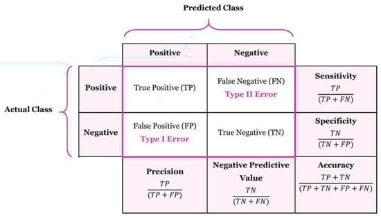
Figure 4.
Confusion matrix.
- Accuracy, a statistical metric, reflects the effectiveness of a binary classifier in correctly identifying a condition. It is calculated as the proportion of correct predictions out of the total number of cases:
- Precision, also known as the “positive predictive value”, measures the ratio of relevant instances among the retrieved instances:
- Sensitivity, recall, hit rate, or true positive rate (TPR), measures the fraction of relevant instances that are correctly retrieved:
- Specificity, or true negative rate (TNR), indicates the fraction of relevant instances that are correctly classified:
- The F1-Score is the harmonic mean of precision and recall:
- The false positive rate represents the probability of incorrectly rejecting the null hypothesis for a given test:
- The area under the curve (ROC-AUC). The Receiver Operating Characteristic (ROC) curve compares sensitivity and specificity. The area under this curve ranges from 0 to 1, where 1 indicates a perfect classifier, 0.5 a completely random classifier, and 0 a classifier that fails to classify any sample correctly. In the formula below, TPR represents the true positive rate, FPR represents the false positive rate, and is a threshold parameter that determines the trade-off between TPR and FPR. The integral symbol denotes the area under the curve, calculated by integrating the TPR with respect to the FPR over the interval [0, 1]:
- Performance measure: This metric is used during hyperparameter tuning to select the best-performing individuals in the population. The scoring metric to be optimized is represented by S, which, in this case, is the ROC-AUC. The train/test splits correspond to the partitions of the cross-validation procedure, and K is a weighting factor that determines the importance of the test results in the final score. This metric functions as a heuristic, aiming to maximize the test value as a function of the difference between the train and test values. This approach helps avoid selecting combinations that exhibit overfitting, where the train result is much higher than the test result, while also favoring combinations with the best overall results. The parameter k controls the relative importance given to the test results versus the difference between train and test results:
2.5. Software Libraries
This section lists the primary software libraries used in this research: Pandas [23] and NumPy [24] for data analysis and processing; imbalanced-learn (imblearn) [25] for class balancing techniques such as SMOTE; scikit-learn (Sklearn) [26] for classification models, pre-processing pipelines, and performance measurement; and XGBoost [27] for gradient boosting algorithms.
3. Results
Our results demonstrate that all machine learning algorithms accurately predicted T21 cases. The machine learning models used for comparison were selected to provide a representative sample of common classification algorithms readily available in the scikit-learn library, supplemented with XGBoost, chosen for its performance, efficiency, and ability to mitigate overfitting. This selection allowed for an evaluation of diverse modeling approaches. Figure 5 illustrates the ROC-AUC metrics obtained by each model during the different stages of training. The differences between the models are minimal, indicating high predictivity across all. Notably, none of the models exhibit significant overfitting or underfitting, as the results from the training, validation, and test sets are consistent with those from the cross-validation (CV) phase. In fact, the test results are slightly higher than the training results, which can be attributed to the proportion of positive samples in the dataset, with the positive samples being the most challenging to predict. The training metrics were calculated on a balanced subset, as previously explained, whereas the test metrics were calculated on the entire sample set, which contains only 0.5% of positive samples; this difference explains the improved test results. Key observations from the model comparison include the following: the SVC model shows slightly lower mean values during the CV phase (0.970) compared to the others; the linear methods, logistic regression (LR) and Stochastic Gradient Descent (SGD), achieve very high results, particularly on the test set (0.980 and 0.979, respectively) but exhibit greater variability during CV, suggesting potentially poorer generalization to new data; the K-Nearest Neighbors (KNN) method performs similarly to the other models (0.982) but also displays more deviation. Among the ensemble models, the decision tree-based methods (Extra Trees (ET) and random forest (RF)) perform slightly worse (0.974 and 0.979, respectively), while the boosting methods, gradient boosting (GB) and XGBoost (XGB), achieve the best ROC-AUC scores (0.982). Finally, the Multi-Layer Perceptron (MLP) model shows comparable results to the other models, with a slightly lower prediction accuracy on the test set (0.975).
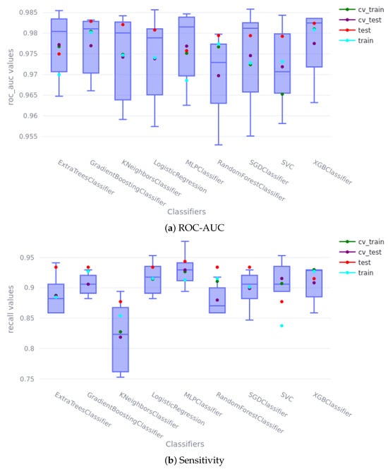
Figure 5.
Cross-validation and train/test scores. In the boxplots, the green and purple dots represent the scores obtained during k-fold CV; the blue and red dots represent the scores obtained during the train/test stage. (a) shows the ROC-AUC score, and (b) shows the sensitivity score.
The hyperparameters selected for each model are presented below; the nomenclature is consistent with that used in the scikit-learn library. The logistic regression (LR) method used elastic net regularization as a penalty, with an l1 ratio of 0.7 and a C value of 5000. The Multi-Layer Perceptron (MLP) employed a 3-hidden-layer network with 4, 2, and 1 neurons in each layer; the learning rate method was ‘adaptive’; the solver was ‘adam’; the activation function was ‘ReLu’; the alpha value was 0.586; batch size was automatic; and early stopping was enabled. The Stochastic Gradient Descent (SGD) method used a constant learning rate with an alpha value of 0.04, an eta0 of 0.006, and the l1 norm. The gradient boosting (GB) method utilized 300 estimators with a maximum depth of 1, a maximum of 0.34 features per node, a minimum of 0.21 samples per leaf, and the friedman_mse method with a learning rate of 0.1. The random forest (RF) method employed the gini criterion with 325 estimators, a maximum depth of 4, and a minimum of 0.01 samples per leaf. The Extra Trees (ET) method also used the gini criterion with 325 estimators, a maximum depth of 6, and a minimum of 0.02 samples per leaf. The Support Vector Classifier (SVC) method used the sigmoid kernel, with gamma values of 0.005 and a C value of 10. Finally, the XGBoost method used 150 estimators with a maximum depth of 1, a subsample ratio of 0.3, an alpha value of 0.145, a lambda value of 0.3, and an eta value of 0.1.
The results indicate that the data used to train the models exhibit well-defined patterns among the different variables and the outcome, enabling highly accurate predictions. The ROC curves for each model are shown in Figure 6; there is minimal difference between most of them, which aligns with the data analysis in Section 2.2.1. Figure 1 and Figure 2 clearly show that high PAPP-A values correlate with negative cases, while high NT and B-HCG values correlate with positive cases. The remaining variables do not appear to have a statistically significant impact on the outcome; however, they do influence the significance of the models. For example, Figure 7 shows the feature importance assigned by each model. Feature importance could not be calculated for every algorithm; therefore, only those that provide this metric are shown. All methods selected only four features: PAPP-A, NT, B-HCG, and age. The other features were discarded because they did not significantly improve the predictions and only introduced noise, reducing model performance. Notably, the linear models (LR and SGD) assign greater importance to PAPP-A and B-HCG compared to the other models, for which NT is the most important variable.
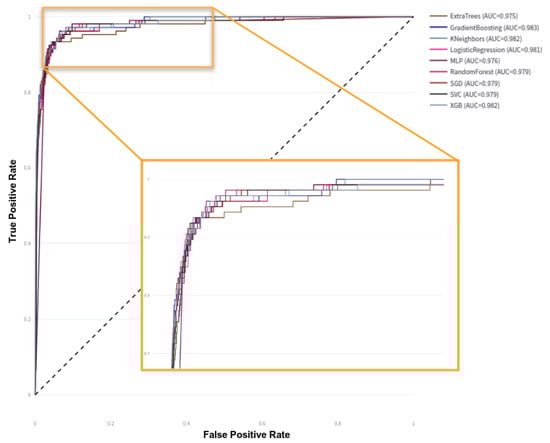
Figure 6.
ROC-AUC curves on test data.
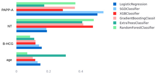
Figure 7.
Model’s feature importance comparison.
Table 3 shows the sensitivity and specificity of each model using two different thresholds. The first is the default threshold of 0.5, where any new individual prediction with a probability greater than 0.5 is classified as positive. The second method, called gmeans, seeks the optimal threshold for a ROC curve by balancing sensitivity and specificity, which is particularly useful for unbalanced classification problems, as is the case here. In a clinical setting, even a seemingly small increase in sensitivity can result in a meaningful reduction in false negatives, ensuring that more affected pregnancies are correctly identified. Similarly, a slight improvement in specificity reduces false positives, minimizing unnecessary anxiety and invasive procedures for low-risk pregnancies. It is also important to acknowledge the inherent trade-off between sensitivity and specificity: models like XGBoost with the gmeans threshold prioritize sensitivity to maximize the detection of positive cases, potentially leading to a slight decrease in specificity; conversely, other models may exhibit higher specificity at the cost of slightly lower sensitivity. The optimal model and threshold depend on the specific clinical priorities and the relative costs of false positives and false negatives.
Table 3.
Model performance comparison with default and gmeans thresholds. This table shows the ROC-AUC, precision–recall AUC, sensitivity, and specificity metrics for each model, using both the default (0.5) and gmeans thresholds.
Finally, Figure 8 presents a confusion matrix with the test data partition of the XGBoost model with the threshold selected by the gmeans method (0.41). It is clear how practically all of the positive cases are classified correctly (0.943 sensitivity), even with the large unbalance problem in the initial dataset. This is largely due to the data balancing techniques used during training. In the case of the negatives, it can be seen to have an equally high predictivity (0.939 specificity).
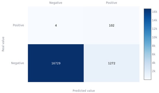
Figure 8.
XGBoost confusion matrix for gmeans threshold on the test partition.
4. Discussion
The early detection of Down syndrome during pregnancy is crucial for parents and healthcare professionals, enabling them to prepare for appropriate care and management of the condition. Machine learning algorithms have been increasingly explored for first-trimester Down syndrome screening, utilizing various diagnostic methods, including maternal serum screening, ultrasound screening, and non-invasive prenatal testing (NIPT). Numerous studies indicate that machine learning algorithms, such as support vector machines (SVMs), random forests, and logistic regression, can effectively predict the risk of Down syndrome with high accuracy, sensitivity, and specificity.
However, it is essential to acknowledge that while machine learning models offer valuable decision support, they are tools to aid, not replace, expert medical judgment. The final diagnosis and clinical decision-making must always remain the responsibility of qualified medical professionals. The models’ output should be interpreted as a risk assessment that physicians use in conjunction with other clinical findings, patient history, and their expertise to guide decisions about further testing or patient management. For example, model-derived risk assessments can help prioritize patients for invasive procedures like amniocentesis or chorionic villus sampling; however, the decision to perform such procedures must be made by a physician in consultation with the patient, carefully weighing individual circumstances and potential risks and benefits.
In this study, the selection of a single superior model is challenging due to the very similar performance metrics across all models. In such cases, the expertise and needs of clinicians become paramount in the decision-making process. Given the unbalanced nature of the problem, accurate identification of positive cases is critical. Even a modest 1% improvement in the hit rate could significantly impact clinical practice. To illustrate, in Spain, with approximately 337,380 births annually, a 1% improvement would translate to identifying roughly 3374 additional cases per year. This improved detection has substantial implications for social, healthcare, and economic considerations. The XGBoost model, using the threshold determined by the gmeans method, was chosen in this study for its optimal balance of sensitivity (0.943) and specificity (0.939), along with a high ROC-AUC value of 0.982.
The performance achieved in this study surpasses that of previous research, including Koivu et al. [18] and Jamshidnezhad et al. [19], which reported lower ROC-AUC values. This improvement can be largely attributed to the hyperparameter optimization implemented in the current study, which employed an algorithm based on genetic optimization. Unlike previous studies that trained their models using a limited set of predetermined hyperparameter values, our approach involved a more extensive, joint optimization. Furthermore, this study benefits from a substantially larger sample size (90,532 samples) compared to Koivu et al. (1850 samples, including 239 positive cases) [18] and He et al. (58,972 samples, with only 27 positive cases) [16].
It is also important to consider the performance of traditional screening methods as a baseline. Traditional first-trimester screening, combining maternal age, nuchal translucency, and biochemical markers (PAPP-A and -hCG), typically achieves a detection rate of approximately 85–90% for trisomy 21, with a false-positive rate of around 5%. While our machine learning models demonstrate comparable or slightly improved overall accuracy (as indicated by ROC-AUC), they offer the potential for more nuanced risk stratification and potentially reduced false-positive rates through optimized thresholds and personalized modeling. This highlights a key advantage of machine learning: the ability to move beyond fixed thresholds and incorporate more complex relationships between variables to refine risk prediction.
A primary limitation of this study is that the data originate solely from Cruces University Hospital in Baracaldo, Spain. This raises concerns about the generalizability of the trained algorithms to other populations. While we hypothesize that the algorithms should be applicable to other populations, particularly Caucasian cohorts (given the features’ worldwide standardization and expected limited differences), generalizability may be more limited for Asiatic or Afro-Caribbean cohorts due to potential genetic variations.
Considering these factors, machine learning algorithms offer several advantages for the early detection of Down syndrome in the first trimester of pregnancy. These advantages include the potential for improved accuracy, sensitivity, and specificity compared to traditional diagnostic methods. Machine learning also facilitates earlier detection and intervention, enabling better preparation for managing the condition. However, challenges and limitations remain, including the need for large and diverse datasets, the potential for bias in the data, and ethical considerations regarding the appropriate use and interpretation of results.
In conclusion, machine learning algorithms show considerable promise for enhancing first-trimester Down syndrome screening, with the potential to improve the accuracy and efficiency of current diagnostic methods. Further research is essential to validate the accuracy and generalizability of these algorithms and to address the associated challenges and limitations.
5. Conclusions
This study investigated the optimization of various machine learning models for predicting the risk of trisomy 21 (T21) in the first trimester of pregnancy. A primary contribution of this work is the application of automated machine learning (AutoML) techniques, specifically tailored to this challenging prediction task.
Our AutoML pipeline incorporated simultaneous feature selection and hyperparameter optimization, utilizing evolutionary algorithms. This approach enabled a more comprehensive exploration of the model space compared to traditional grid search or random search methods. Hyperparameter optimization proved crucial for maximizing model performance, particularly given the unbalanced nature of the real-world dataset, where negative cases significantly outnumbered positive cases.
The optimization process aimed to balance the competing objectives of maximizing both sensitivity and specificity, a critical consideration in clinical applications. Employing a custom performance metric during hyperparameter tuning effectively mitigated overfitting and ensured robust generalization.
Although all models achieved high predictive accuracy due to the quality and size of the dataset, subtle differences in their performance characteristics were carefully analyzed. Ultimately, the XGBoost model was selected as the most suitable for clinical use, demonstrating a favorable trade-off between sensitivity and specificity.
Future research should investigate the generalizability of these optimized models to other diverse populations and explore the integration of additional data modalities, such as cell-free DNA, to further enhance prediction accuracy. Furthermore, explainability techniques could be applied to the models to provide clinicians with greater insight into the factors influencing individual risk predictions.
Author Contributions
Conceptualization, E.A. and J.B.; methodology, E.A.; software, E.A.; validation, E.A., J.B. and A.B.; formal analysis, E.A.; investigation, E.A., J.B. and I.G.; resources, A.B.; data curation, E.A.; writing—original draft preparation, E.A.; writing—review and editing, A.B. and I.G.; visualization, E.A.; supervision, A.B.; project administration, E.A.; funding acquisition, A.B. All authors have read and agreed to the published version of the manuscript.
Funding
This work was partially funded by grant PID2021-123087OB-I00 funded by the Spanish Ministry of Science, Innovation and Universities—National Research Agency (MCIN/AEI/10.13039/501100011033), the European Regional Development Fund (ERDF), and by the Department of Education, Universities and Research of the Basque Government (ADIAN, IT-1437-22).
Institutional Review Board Statement
This study was conducted in accordance with the Declaration of Helsinki and approved by the Institutional Review Board (or Ethics Committee) of Osakidetza (protocol code CEI 21/03 and date of approval 28 January 2022).
Informed Consent Statement
Informed consent was obtained from all subjects involved in this study.
Data Availability Statement
Restrictions apply to the availability of these data. The data were obtained from Osakidetza, the Basque Country public health service, and are available with the permission of an ethics committee.
Acknowledgments
The authors thank the obstetrics and gynecology service of the Cruces University Hospital for their help in cleaning the data, their comments to initially understand the problem, and their contribution to the validation of the models thanks to their clinical knowledge, which has allowed us to select the best models based on clinical needs. We also thank the Government of the Basque Country for funding the NONA project under the ELKARTEK framework, thanks to which we have been able to collaborate jointly with Osakidetza and produce this publication.
Conflicts of Interest
The authors declare no conflicts of interest.
References
- Asim, A.; Kumar, A.; Muthuswamy, S.; Jain, S.; Agarwal, S. Down syndrome: An insight of the disease. J. Biomed. Sci. 2015, 22, 41. [Google Scholar] [CrossRef] [PubMed]
- Mai, C.T.; Isenburg, J.L.; Canfield, M.A.; Meyer, R.E.; Correa, A.; Alverson, C.J.; Lupo, P.J.; Riehle-Colarusso, T.; Cho, S.J.; Aggarwal, D.; et al. National population-based estimates for major birth defects, 2010–2014. Birth Defects Res. 2019, 111, 1420–1435. [Google Scholar] [CrossRef] [PubMed]
- Loane, M.; Morris, J.K.; Addor, M.C.; Arriola, L.; Budd, J.; Doray, B.; Garne, E.; Gatt, M.; Haeusler, M.; Khoshnood, B.; et al. Twenty-year trends in the prevalence of Down syndrome and other trisomies in Europe: Impact of maternal age and prenatal screening. Eur. J. Hum. Genet. 2013, 21, 27–33. [Google Scholar] [CrossRef] [PubMed]
- Akhtar, F.; Bokhari, S.R.A. Down Syndrome (Trisomy 21). In StatPearls; StatPearls Publishing: Treasure Island, FL, USA, 2019. [Google Scholar]
- Canick, J. Prenatal screening for trisomy 21: Recent advances and guidelines. Clin. Chem. Lab. Med. 2012, 50, 1003–1008. [Google Scholar] [CrossRef]
- Huang, T.; Gibbons, C.; Rashid, S.; Priston, M.K.; Bedford, H.M.; Mak-Tam, E.; Meschino, W.S. Prenatal screening for trisomy 21: A comparative performance and cost analysis of different screening strategies. BMC Pregnancy Childbirth 2020, 20, 713. [Google Scholar] [CrossRef]
- Alldred, S.K.; Takwoingi, Y.; Guo, B.; Pennant, M.; Deeks, J.J.; Neilson, J.P.; Alfirevic, Z.; Pregnancy, C.; Group, C. First trimester serum tests for Down’s syndrome screening. Cochrane Database Syst. Rev. 1996, 2015, CD011975. [Google Scholar] [CrossRef]
- Spencer, K.; Souter, V.; Tul, N.; Snijders, R.; Nicolaides, K.H. A screening program for trisomy 21 at 10–14 weeks using fetal nuchal translucency, maternal serum free beta-human chorionic gonadotropin and pregnancy-associated plasma protein-A. Ultrasound Obstet. Gynecol. 1999, 13, 231–237. [Google Scholar] [CrossRef]
- Guibourdenche, J.; Leguy, M.C.; Pidoux, G.; Hebert-Schuster, M.; Laguillier, C.; Anselem, O.; Grangé, G.; Bonnet, F.; Tsatsaris, V. Biochemical Screening for Fetal Trisomy 21: Pathophysiology of Maternal Serum Markers and Involvement of the Placenta. Int. J. Mol. Sci. 2023, 24, 7669. [Google Scholar] [CrossRef]
- Cuckle, H.S.; van Lith, J.M. Appropriate biochemical parameters in first-trimester screening for Down syndrome. Prenat. Diagn. 1999, 19, 505–512. [Google Scholar] [CrossRef]
- Royston, P.; Thompson, S.G. Model-based screening by risk with application to Down’s syndrome. Stat. Med. 1992, 11, 257–268. [Google Scholar] [CrossRef]
- Coppedè, F. Risk factors for Down syndrome. Arch. Toxicol. 2016, 90, 2917–2929. [Google Scholar] [CrossRef] [PubMed]
- Sandin, S.; Hultman, C.M.; Kolevzon, A.; Gross, R.; MacCabe, J.H.; Reichenberg, A. Advancing maternal age is associated with increasing risk for autism: A review and meta-analysis. J. Am. Acad. Child Adolesc. Psychiatry 2012, 51, 477–486. [Google Scholar] [CrossRef] [PubMed]
- Hildebrand, E.; Källén, B.; Josefsson, A.; Gottvall, T.; Blomberg, M. Maternal obesity and risk of Down syndrome in the offspring. Prenat. Diagn. 2014, 34, 310–315. [Google Scholar] [CrossRef] [PubMed]
- Pitukkijronnakorn, S.; Promsonthi, P.; Panburana, P.; Udomsubpayakul, U.; Chittacharoen, A. Fetal loss associated with second trimester amniocentesis. Arch. Gynecol. Obstet. 2011, 284, 793–797. [Google Scholar] [CrossRef]
- He, F.; Lin, B.; Mou, K.; Jin, L.; Liu, J. A machine learning model for the prediction of down syndrome in second trimester antenatal screening. Clin. Chim. Acta 2021, 521, 206–211. [Google Scholar] [CrossRef]
- Ramanathan, S.; Sangeetha, M.; Talwai, S.; Natarajan, S. Probabilistic determination of down’s syndrome using machine learning techniques. In Proceedings of the 2018 International Conference on Advances in Computing, Communications and Informatics (ICACCI), Bangalore, India, 19–22 September 2018; IEEE: Piscataway, NJ, USA, 2018; pp. 126–132. [Google Scholar]
- Koivu, A.; Korpimäki, T.; Kivelä, P.; Pahikkala, T.; Sairanen, M. Evaluation of machine learning algorithms for improved risk assessment for Down’s syndrome. Comput. Biol. Med. 2018, 98, 1–7. [Google Scholar] [CrossRef]
- Jamshidnezhad, A.; Hosseini, S.M.; Mohammadi-Asl, J.; Mahmudi, M. An intelligent prenatal screening system for the prediction of Trisomy-21. Inform. Med. Unlocked 2021, 24, 100625. [Google Scholar] [CrossRef]
- Agathokleous, M.; Chaveeva, P.; Poon, L.C.Y.; Kosinski, P.; Nicolaides, K.H. Meta-analysis of second-trimester markers for trisomy 21. Ultrasound Obstet. Gynecol. 2013, 41, 247–261. [Google Scholar] [CrossRef]
- Grubbs, F.E. Sample Criteria for Testing Outlying Observations. Ann. Math. Stat. 1950, 21, 27–58. [Google Scholar] [CrossRef]
- Chawla, N.V.; Bowyer, K.W.; Hall, L.O.; Kegelmeyer, W.P. SMOTE: Synthetic Minority Over-sampling Technique. J. Artif. Intell. Res. 2002, 16, 321–357. [Google Scholar] [CrossRef]
- Mckinney, W. Data Structures for Statistical Computing in Python. In Proceedings of the 9th Python in Science Conference, Austin, TX, USA, 28 June–3 July 2010. [Google Scholar]
- Harris, C.R.; Millman, K.J.; van der Walt, S.J.; Gommers, R.; Virtanen, P.; Cournapeau, D.; Wieser, E.; Taylor, J.; Berg, S.; Smith, N.J.; et al. Array programming with NumPy. Nature 2020, 585, 357–362. [Google Scholar] [CrossRef] [PubMed]
- Lemaitre, G.; Nogueira, F.; Aridas, C.K. Imbalanced-learn: A Python Toolbox to Tackle the Curse of Imbalanced Datasets in Machine Learning. arXiv 2016, arXiv:1609.06570. [Google Scholar]
- Pedregosa, F.; Varoquaux, G.; Gramfort, A.; Michel, V.; Thirion, B.; Grisel, O.; Blondel, M.; Prettenhofer, P.; Weiss, R.; Dubourg, V.; et al. Scikit-learn: Machine Learning in Python. J. Mach. Learn. Res. 2011, 12, 2825–2830. [Google Scholar]
- Chen, T.; Guestrin, C. XGBoost: A Scalable Tree Boosting System. In Proceedings of the 22nd ACM SIGKDD International Conference on Knowledge Discovery and Data Mining, San Francisco, CA, USA, 13–17 August 2016; ACM: New York, NY, USA, 2016. [Google Scholar] [CrossRef]
Disclaimer/Publisher’s Note: The statements, opinions and data contained in all publications are solely those of the individual author(s) and contributor(s) and not of MDPI and/or the editor(s). MDPI and/or the editor(s) disclaim responsibility for any injury to people or property resulting from any ideas, methods, instructions or products referred to in the content. |
© 2025 by the authors. Licensee MDPI, Basel, Switzerland. This article is an open access article distributed under the terms and conditions of the Creative Commons Attribution (CC BY) license (https://creativecommons.org/licenses/by/4.0/).