Article

Health Assessment of Rolling Bearings Based on Multivariate State Estimation and Reliability Analysis

1
School of Mechanical Engineering, Southwest Jiaotong University, Chengdu 610031, China
2
Technology and Equipment of Rail Transit Operation and Maintenance Key Laboratory of Sichuan Province, Chengdu 610031, China
*
Author to whom correspondence should be addressed.
Appl. Sci. 2025, 15(10), 5396; https://doi.org/10.3390/app15105396
Submission received: 23 March 2025 / Revised: 27 April 2025 / Accepted: 9 May 2025 / Published: 12 May 2025

Abstract

:
Rolling bearing is an indispensable part of mechanical rotating parts, which plays an important role in reducing friction and ensuring the rotation accuracy of rotating parts. It is necessary to carry out a health assessment of the bearing. Current health assessment methods for rolling bearings only extract strongly related feature indicators and input them into the health assessment model without considering the profound impact external conditions have on the fluctuation of feature indicators, which will lead to an inaccurate health assessment. Besides, most methods evaluating the health of rolling bearings only consider the real-time index data but do not make full use of bearing maintenance data for reliability modeling and analysis, actually reducing the hierarchy and rationality of the health assessment. Therefore, this paper combines multivariate state estimation (MSET) and reliability analysis to evaluate the health of rolling bearings. Firstly, the health baseline of the rolling bearing under multi-speed conditions is established based on MSET, which collects the history health data of rolling bearings under various working conditions and learns the impact of working conditions on health data. Subsequently, Mahalanobis distance is used to measure the degree of deviation from the health baseline, and calculated Mahalanobis distance is input into the health mapping function to get the initial health score. Finally, combined with the reliability analysis correcting the initial score, the final health score is obtained, which can provide data support for intelligent operation and maintenance and a decision-making basis for equipment maintenance. The proposed health assessment method is validated using the bearing dataset from Case Western Reserve University and historical failure data of rolling bearings. The proposed method reduces speed-related influences in bearing health evaluation, dynamically adjusting the health assessment result through the reliability model to track performance degradation throughout the bearing’s service life.

1. Introduction

As a key part of large complex mechanical components, the rolling bearing plays a vital role in the mechanical system. Its main functions include supporting the mechanical rotating body, reducing the friction resistance during the movement of the rotating body, and ensuring its rotation accuracy [1]. In the train bogie, rolling bearings are mainly divided into motor bearings, gearbox bearings and axle box bearings according to their different installation positions. The motor bearing is used to support the rotation of the motor shaft, the gearbox bearing supports the movement of the gearbox shaft, and the axle box bearing directly supports the rotation of the wheel axle. These bearings work together to ensure the stability, smoothness, and ride comfort of the train during high-speed operation, which is an important guarantee of the train’s quality. However, the service environment of rolling bearings is usually very harsh, and the bearings not only need to withstand the huge impact load from wheel-rail contact during service but also to deal with the centrifugal force brought by high-speed rotation, temperature changes, fluctuations in lubrication conditions and the intrusion of external pollutants such as dust and moisture. These factors work together to make rolling bearings prone to wear, fatigue cracks, spalling and other failures during long-term service. Once a bearing malfunctions, it can cause abnormal vibrations and noise at the very least, and at worst, it may lead to severe incidents such as equipment damage or train derailments, resulting in significant economic losses and even posing a threat to the safety of passengers and crew. Therefore, it is particularly important to carry out real-time monitoring and health assessment on the rolling bearings, which can advance the fault detection threshold, reduce the risk of unplanned downtime of equipment, and significantly extend the service life of bearings. Through advanced sensing technology, physical parameters such as vibration and temperature during bearing operation can be collected in real-time. Combined with the actual situation, the characteristic index of vibration acceleration has become the most commonly used monitoring parameter because of its high sensitivity, easy collection and processing, and the bearing health assessment based on the characteristic indicators of vibration, which is the most common.
The development of fault diagnosis technology began in the 1960s [2]. The bearing fault diagnosis method based on signal processing technology was widely used. Braun [3] used time-domain synchronous equalization to improve the periodic components of oscillating signals, thereby enhancing the accuracy of diagnosing faulty bearings. Chaturvedi [4] applied adaptive noise reduction to the diagnosis of the slight weakness fault of the bearing. Tan [5] applied the method combining variable-scale stochastic resonance and weighted kurtosis index to the diagnosis of fault signals. The basic process is to first extract the multi-source parameters of key components, such as vibration, temperature and other parameters, for real-time collection and analysis to determine whether their service status is normal. If the monitoring parameters exceed the threshold or show abnormal characteristics, the fault diagnosis mechanism is triggered. At present, the in-transit monitoring of rolling bearings is mostly completed by setting a fixed fault warning threshold, but in the actual monitoring process, there are often false positives and missed positives [6]. This is because the degradation and failure of the physical properties of the bearing will aggravate the vibration, and the amplitude of vibration acceleration will increase. However, when the external working conditions change during service, such as the speed increases, the vibration amplitude will also increase, which will affect the evaluation of the bearing performance. Therefore, in the health assessment of rolling bearings, reducing the impact of varying operating conditions and improving the accuracy of health assessment are critical and challenging focuses of current research [7].
With the development of the technology, an increasing number of neural network models are being applied to the health assessment of rolling bearings. Zhang [8] proposed a performance degradation evaluation method based on long short-term memory and recurrent neural networks to evaluate the real-time running state of bearings. Shao [9] proposed a self-organizing feature mapping (SOM) neural network to assess the health state of the gearbox rolling bearing. The neural network model can automatically extract complex features and has strong nonlinear modeling capabilities, but it requires a large amount of high-quality labeled data, which is hard to obtain and has poor model interpretability.
Probabilistic models are also commonly used in the health assessment of rolling bearings. Yao [10] used the hidden Markov dynamic pattern recognition theory to evaluate the health of rolling bearings. Zhang [11] used the Gaussian mixture model to calculate the likelihood probability as a health factor characterizing component degradation. Based on Bayesian theory, Gao [12] quantified the overlap degree between the features of the state space to be evaluated and the health state space as the health indicator of the bearing degradation state so as to realize the state degradation assessment of rolling bearings. The probabilistic model has strong interpretability and can clearly describe the probabilistic relationship between the bearing state and the monitoring data. However, probabilistic models have relatively poor robustness and are highly sensitive to data quality and distribution assumptions. When the data contains noise or deviates from the assumed distribution, the performance of bearings evaluated by the model may significantly degrade.
The multivariate state estimation technique (MSET) is a non-parametric data-driven model [13]. By taking the historical health data of the equipment as input, the model can build the historical memory matrix of MSET, which contains health observation vectors under different working conditions, learning the health law and service characteristics of the equipment. When a new observation vector is input, it will be matched with vectors under all working conditions in the historical memory matrix, and the health vector output under the most similar working conditions will be set as the baseline to achieve the effect of removing the influence of working conditions. When the new observed data deviates from the health space, the performance of the equipment deteriorates [14].
Since MSET can establish a health baseline for mechanical equipment under multiple operating conditions without relying on hard-to-obtain fault data, and due to its strong robustness, it has been widely applied in the field of mechanical equipment health assessment [15]. Wang [16] proposed a wind turbine condition monitoring method based on MSET, which aims to achieve fault early warning of wind turbine components. Zeng [17] proposed an improved MSET with a composite operator (CO-MSET) for electro-mechanical actuators’ health indicator extraction. Sun [18] established a fault warning model for induced draft fans by using MSET. These studies established a health baseline based on the health data of the mechanical equipment, which is convenient for the subsequent health assessment and maintenance strategy formulation.
Owing to the characteristics of MSET, both the input observation vector and the output estimation vector (health baseline) are typically high-dimensional vectors encompassing multiple performance parameters. This allows the algorithm to construct a high-dimensional state-space model, thereby more accurately characterizing the complex nonlinear relationships between bearing operating states and multi-sensor data. However, in current research utilizing MSET for mechanical equipment health assessment, Euclidean distance is commonly integrated with MSET to quantify the deviation between the observation vector and the estimation vectors (the health baseline). However, Euclidean distance fails to effectively eliminate the influence of dimensional differences when processing multidimensional parameters with varying units [19], and errors may be introduced into the deviation measurement, consequently compromising the accuracy and reliability of health assessment. In addition, existing research on the health assessment of mechanical equipment primarily focuses on real-time data, often neglecting to incorporate historical maintenance records as a reference dimension into the health assessment framework. As equipment ages, its performance naturally degrades, and the probability of failure increases. By analyzing the time between failures of failed equipment in similar working conditions and establishing the reliability model to assess the equipment’s failure probability, the health assessment can be dynamically corrected based on the reliability analysis. This approach ensures that the health assessment results more precisely reflect the actual performance degradation of the equipment.
To address the aforementioned issues, this paper proposes a rolling bearing health assessment method integrating MSET and reliability analysis. The framework comprises four key phases: (1) Constructing condition-specific health baselines through MSET-based historical memory matrix optimization; (2) Adopting Mahalanobis distance metric for multidimensional degradation quantification; (3) Establishing health score mapping through nonlinear function design; (4) Implementing reliability-driven dynamic correction with service mileage integration. The principal advances distinguishing this research include:
  • A condition-robust deviation quantification mechanism that synergizes MSET’s nonlinear modeling with Mahalanobis distance’s covariance sensitivity, resolving Euclidean metric’s limitations in handling correlated multivariate bearing parameters and speed variation interference.
  • A reliability-informed health evaluation paradigm that dynamically calibrates degradation assessment through statistical failure patterns, achieving service-mileage adaptive precision improvement beyond fixed-parameter assessment frameworks.
  • Comprehensive validation through Case Western Reserve University bearing datasets demonstrates two advantages: (1) Inherent resistance to rotational speed fluctuation interference during operation. (2) Physically consistent monotonic degradation progression mapping across fault evolution phases.
The remaining sections are structured as follows: Section 2 details MSET-based baseline modeling, Section 3 presents the reliability-integrated correction methodology, Section 4 validates the approach through CWRU experimental analysis, and Section 5 concludes with a research outlook.

2. Modeling of Initial Health Assessment Based on MSET

2.1. Select Feature Indicators

Extracting the bearing vibration acceleration characteristic indicator for analysis is an important means of monitoring the bearing health state. The vibration acceleration signal itself contains a wealth of fault information, which can sensitively reflect the subtle changes in bearing performance, such as internal bearing scratches, cracks, electrical erosion, spalling and other faults, which can be reflected in the vibration acceleration characteristic indicators [20]. Each characteristic indicator of vibration acceleration has its own physical significance, and its sensitivity to different types of faults is different. Considering the calculation efficiency of the model and the physical meaning of each characteristic indicator, three indicators of vibration acceleration, namely root mean square value, peak value and kurtosis, are selected to characterize the degradation trend of bearing performance. These three indicators—vibration peak, kurtosis and RMS collectively capture distinct degradation signatures across bearing lifespan. They exhibit strong correlations with progressive performance deterioration: peak amplitude directly links to localized defects, kurtosis sensitizes to early-stage micro-faults, and RMS correlates with cumulative wear severity, thereby enabling multi-stage degradation characterization. The physical meanings of these three characteristics are as follows:
The root-mean-square value is used to measure the average strength of vibration signals. This value reflects the energy level of the vibration signal over a certain time or frequency band, expressed as follows:
x r m s = 1 n i = 1 n x i 2
The peak value refers to the single-peak maximum value of the vibration waveform, which reflects the maximum impact force suffered during the vibration process. Once the peak value is abnormally large, it indicates that the performance of the equipment has declined, which needs to be paid attention to by operation and maintenance. The expression is shown as follows:
x p = max x i
Kurtosis represents the sharpness of the vibration signal waveform and measures the tail thickness of the data distribution, which refers to the frequency with which outliers occur. When running without fault, the amplitude distribution of the vibration signal is close to the normal distribution. With the occurrence and development of the fault, the probability density of the large peak value of the vibration signal increases, the distribution of the signal amplitude deviates from the normal distribution, and the kurtosis value also increases. The expression is as follows:
K = i = 1 n ( x i x ¯ ) 4 ( n 1 ) σ 4

2.2. Establish Health Baseline Based on MSET

MSET is a non-parametric modeling method first proposed by Argonne National Laboratory in the United States and has been successfully applied to nuclear power plant equipment parameter degradation detection, power system state estimation, electronic equipment life prediction and other fields [21,22,23,24].
MSET is a nonlinear multivariate prediction and diagnosis technology. In essence, MSET is based on the input of the normal operation data of the equipment under historical working conditions, and then the health rule is learned from the normal operation data of the multi-working conditions through the algorithm to establish the health model of the equipment. In this way, when the observation data to be evaluated is input into the model, it calculates and estimates the data during normal operation based on the analysis and comparison of actual monitoring data and the health data during normal operation of the equipment and outputs the health data estimated by the algorithm under the current working condition as the benchmark for the subsequent health assessment of the equipment [25]. The specific application steps of the algorithm are as follows:
First, select n feature indicators that characterize the health state of the component, which can be expressed as x j , j = 1 , 2 , , n . Then, record the sequence of feature indicators of the component at the moment t j as the observation vector X ( t j ) . The expression is as follows:
X ( t j ) = [ x 1 ( t j ) x 2 ( t j ) x n ( t j ) ]
Then, the observation vectors of the component’s historical health status are collected to establish the historical memory matrix D , as is shown in Equation (5). The historical matrix D R n × m , where each column X ( t j ) = [ x 1 ( t j ) x 2 ( t j ) x n ( t j ) ] T represents the multi-feature observation vector t j with n selected indicators, and each row captures the temporal evolution of the i -th indicator.
D = [ X ( t 1 ) X ( t 2 ) X ( t m ) ] = x 1 ( t 1 ) x 1 ( t 2 ) x 1 ( t m ) x 2 ( t 1 ) x 2 ( t 2 ) x 2 ( t m ) x n ( t 1 ) x n ( t n ) x n ( t m )
The observation vectors of the normal operations under all working conditions are input into the model to construct the memory matrix D . MSET is a data-driven model. The larger the data of the memory matrix and the more working conditions it covers, the more accurate the output estimation vector will be. Constructing the historical memory matrix is a crucial step of MSET, and it is the basis for the subsequent algorithm to learn the normal operation rules of the memory equipment and match the working conditions.
Next, the current observation vector of the device to be evaluated X o b s is input into MSET, the working condition is matched with the historical memory matrix D , and the estimated vector X e s t is output after calculation. In the process of condition matching, the model will generate a corresponding m-dimension weight vector W for each observation vector. The expression is as follows:
W = [ w 1 w 2 w m ] T
The weight vector W represents the degree of similarity between the observation vector X o b s and the m-column historical memory matrix D . Therefore, the estimation vector X e s t is equal to the historical memory matrix D multiplied linearly by the weight vector W , calculated as follows:
X e s t = D W = w 1 X ( t 1 ) + w 2 X ( t 2 ) + + w m X ( t m )
Given the observation vector X o b s and the estimation vector X e s t , the residual ε can be calculated by subtracting the two. The expression is as follows:
ε = X e s t X o b s
By minimizing the residual vector ε and deriving the weight vector W using the least square method, the expression is as follows:
ε 2 = X o b s X e s t 2 = 0
Further expand the operation:
F ( w ) = i = 1 n ε i 2 = ε T ε = ( X o b s D W ) T ( X o b s D W ) = i = 1 n ( X o b s ( i ) j = 1 m w j D i j ) 2
The partial derivative of w k , k = 1 , 2 , , m is obtained from F ( w ) and set to 0, which is calculated as follows:
F ( w ) w k = 2 i = 1 n ( X o b s ( i ) j = 1 m w i D i j ) D i k = 0
i = 1 n X o b s ( i ) D i k = i = 1 n i = 1 m w j D i j D i k = j = 1 m ( i = 1 n D i j D i k ) w j
Convert the above equation to matrix form:
D T · D · W = D T · X o b s
W = ( D T · D ) 1 ( D T · X o b s )
According to Equation (14), D T · D invertibility is a prerequisite for the existence of a weight vector W , and a necessary but not sufficient condition for invertibility is that the number of columns D is less than the number of rows D [26]. In fact, in order to make the calculation accuracy of MSET high, the memory matrix needs to include as much as possible the historical observation vector that the equipment runs normally under all working conditions. Therefore, the number of columns of the memory matrix is bound to be greater than the number of rows, so the weight vector cannot be calculated by dot multiplication. Nonlinear operators can be used to solve such problems, and the matrix product can be replaced by nonlinear operators to avoid the irreversible problem of matrix multiplication. Therefore, the matrix-vector expression is:
W = ( D T D ) 1 ( D T X o b s )
where is the symbol of nonlinear operation, Euclidean distance is chosen as the nonlinear operator between vectors, defined as the following equation:
( X , Y ) = i = 1 n ( x i y i ) 2
where X , Y refer to vectors.
The higher the similarity between the observation vector X o b s and the vector X j , j = 1 , 2 , , m in the historical memory matrix D is, the greater the corresponding weight w j , j = 12 , , m will be, and the weight vector W can be calculated from this.
Substitute the weight vector W into Equation (7) to calculate the estimation vector X e s t , and simplify it, as shown as follows:
X e s t = D ( D T D ) 1 ( D T X o b s )
The estimation vector as the output of MSET represents the data condition predicted by the model when the equipment is in a normal state under the current working condition to be evaluated and can be used as the health benchmark of the current equipment operation condition. The greater the deviation between the observation vector and the estimation vector is, the further the equipment deviates from the health benchmark. When the deviation between the observation vector and the estimation vector is small, it indicates that the device is currently in a healthy state or that the degree of performance degradation is small. By condition matching, the multivariate state estimation method outputs the estimation vector after removing the influence of the condition. By quantifying the deviation degree between the observation vector and the estimation vector, combined with the health mapping equation, the purpose of evaluating the current equipment’s health state is finally achieved.

2.3. Deviation Distance Measurement Based on Mahalanobis Distance

The performance state of rolling bearings can be characterized by vibration characteristics, and the statistical distribution of the index data space in the normal state is different from that in the degraded or faulty state. By quantifying the degree of deviation, the degree of performance degradation of rolling bearings can be measured. The degree of deviation is positively correlated with the degree of performance degradation. The greater the degree of deviation of the current state indicator data from the health baseline, the greater the degree of performance degradation.
Mahalanobis distance was developed by Indian statistician Mahalanobis to measure the distance between a sample point and a data distribution. Multidimensional data can take into account the covariance between the dimensions, which can better reflect the true distribution of the data. The Mahalanobis distance expression is as follows:
d ( x , y ) = ( x y ) T X 1 ( x y )
where x , y are two samples that follow the same distribution, which in this paper respectively refer to the observation vector X o b s and the estimation vector X e s t X 1 represents the covariance matrix of the reference sample, where is the covariance of the historical memory matrix D .
The observation vector is composed of the root mean square value, the peak value and the kurtosis, representing the equipment health state from three dimensions. The data units and value ranges of the three dimensions are different, and the traditional Euclidean distance calculation of the distance between the two data will be affected by the different value ranges of the multidimensional data and the correlation of the non-independent distribution between the dimensions, thus affecting the accuracy of the distance measurement results. Different from the traditional Euclidean distance, Mahalanobis distance not only considers the dimension of each dimension of data but also the correlation between them, which makes Mahalanobis distance more effective in the processing of multidimensional data with correlation [27]. The Mahalanobis distance first rotates the data of each dimension according to the principal component to make the dimensions independent of each other, and then the distance is calculated after data standardization to make the measurement result more accurate.
After calculating the distance of the observation vector deviating from the estimation vector through the Mahalanobis distance, input the subsequent health mapping function to evaluate the health state of the rolling bearing.

2.4. Health Mapping Function

Choose the exponential function as the mapping equation for the performance deviation distance of the rolling bearing, as shown as follows:
    H S = 100 × e k × d ( X o b s , X e s t ) T T = a v e r ( d ( X o b s _ n o r m , X e s t _ n o r m ) )
where H S refers to the current health score of the rolling bearing mapped by the health function, k refers to the sensitivity coefficient, and d ( X o b s , X e s t ) refers to the Mahalanobis distance between the observation vector and the estimation vector of the data to be evaluated. T refers to the distance that the generally normal data in the memory matrix D deviates from the normal data space, serving as a threshold. Its value is calculated by the Mahalanobis distance between the observed vector and the estimated vector of the data extracted at every 20 points in the memory matrix D , and then the average value is taken as T . X o b s _ n o r m and X e s t _ n o r m , respectively, refer to the observation vector and the estimation vector of the extracted data. Here k is set as 0.0035.

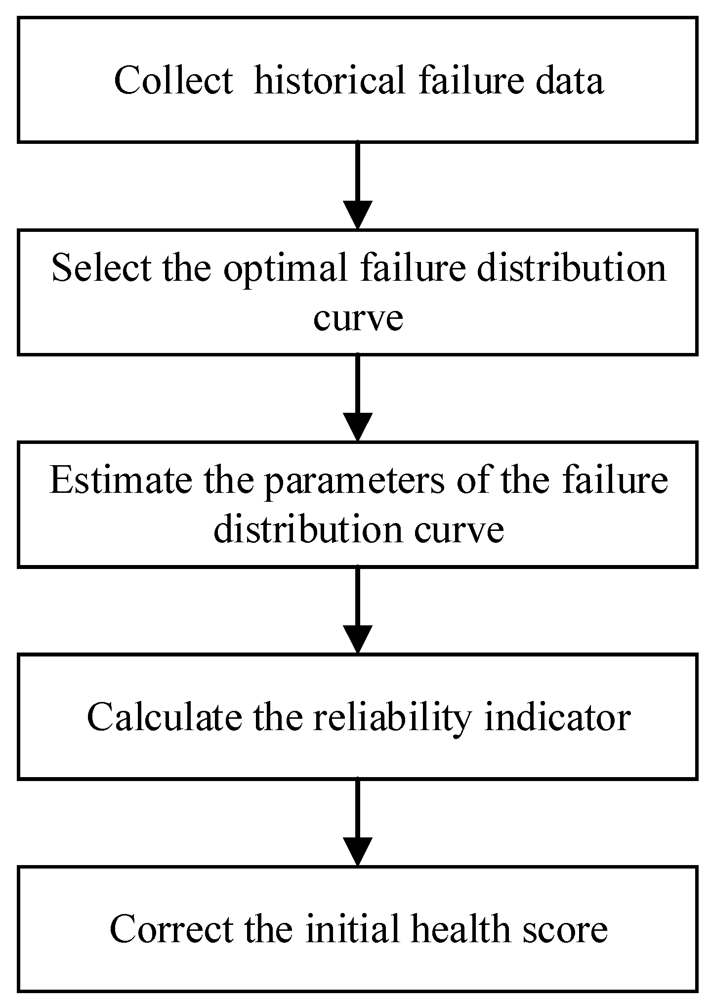
3. Health Score Correction Based on the Reliability Model

The reliability of equipment is defined as its ability to perform specified functions under designated conditions and within a specified time frame [28]. It serves as an indicator for evaluating the in-service performance of equipment, reflecting the probability that the equipment will maintain normal operation during actual service. Reliability is closely related to the design and manufacturing processes prior to the equipment’s delivery, as well as the actual service environment and duration post-delivery. Once the equipment is put into use, its performance tends to degrade over time due to aging and the influence of external operating conditions. As the service time increases, the likelihood of failure rises, leading to a decline in reliability, which reflects the health status of the equipment in the aspect of service time. By collecting historical failure data from the same type of equipment under similar operating conditions and selecting evaluation criteria, the reliability model that best aligns with the equipment’s performance degradation can be developed to assess its reliability. On the basis of the initial health assessment of the rolling bearing, further consideration of the rolling bearing’ historical failure information is incorporated. Reliability analysis is used to adjust the initial health assessment, integrating multi-source data to provide a more comprehensive and reliable assessment of bearing health from multiple perspectives, thereby better guiding maintenance operations. The flowchart of health score correction based on the reliability model is illustrated in Figure 1.

3.1. Reliability Indicators

Reliability indicators include cumulative failure probability F ( t ) , failure probability density f ( t ) , reliability R ( t ) , and failure rate λ ( t ) . Their definitions are shown below:
Cumulative failure probability F ( t ) is defined as the probability that a device fails to perform its specified function (i.e., experiences a failure) under specified conditions before a given time t . It is also referred to as uncertainty. The cumulative failure probability failure distribution curve serves as the foundation for describing the random failure patterns of equipment and conducting reliability analysis. Its definition is expressed as follows:
F ( t ) = P ( T t )
where T represents the time of equipment failure. It is important to note that t is a generalized concept and is not limited solely to the service time of the equipment. Instead, it depends on the specific object of analysis and the application scenario. When the reliability analysis focuses on equipment in the transportation sector, the operational mileage is often used as a unit for reliability analysis [29].
Failure probability density f ( t ) is defined as the probability that a device fails to perform its specified function under specified conditions at a unit moment. Assuming f ( t ) is smooth, if the sample size is continuously increased while the interval length is reduced, the frequency of samples falling within the interval covering a specific point will decrease and tend toward zero as the interval length shrinks. However, the ratio of frequency to interval length will gradually converge to a fixed value, which is the failure probability density f ( t ) . The curve formed by all such f ( t ) values is called the failure probability density curve, representing the likelihood of the random variable occurring within a unit interval. Therefore, the definition of f ( t ) is expressed as follows:
f ( t ) = d F ( t ) d t
Reliability R ( t ) is defined as the probability that a device can perform its specified function under specified conditions within a given time t , and it can be expressed as:
R ( t ) = P ( T > t )
where T represents the time of equipment failure. From the definition, it can be seen that reliability R ( t ) and cumulative failure probability F ( t ) are complementary. Therefore, R ( t ) can be derived from F ( t ) as follows:
R ( t ) = 1 F ( t )
Failure Rate λ ( t ) is defined as the probability that a device which has not failed by time t under specified conditions, will fail in the unit time interval immediately following t . It describes the dynamic characteristics of the likelihood of failure, and its definition is expressed as follows:
λ ( t ) = lim Δ t 0 P ( t < T t + Δ t T > t ) Δ t
Based its definition, failure rate λ ( t ) can be derived from failure probability density f ( t ) and reliability R ( t ) as follows:
λ ( t ) = f ( t ) R ( t )

3.2. Commonly Used Failure Distribution Curves

The time to failure of an individual device is a random variable. For a single device in service, its time to failure or mileage to failure is unknown; however, for devices of the same type operating under identical service conditions, the time to failure or mileage to failure follows a determinable distribution pattern, which can be derived by collecting statistical failure data. Suppose n samples are randomly drawn from the population. Although the sampling results are random, the frequency of samples within different intervals varies. The likelihood of a random variable taking values within specific intervals represents the intuitive meaning of “distribution”. In practical applications, it is always assumed that the failure time distribution of the population exists and is determinable. Since an individual belongs to this population, in the absence of any prior information, the failure time of the individual is a random variable that follows this distribution [28].
In reliability analysis, commonly used failure distributions include normal distribution, log-normal distribution, exponential distribution, two-parameter Weibull distribution and gamma distribution. The specific type of distribution is often unrelated to the type of product but is instead associated with the type of stress applied, the failure mechanism, and the failure mode. Therefore, the following sections will introduce the probability density f ( t ) , the cumulative failure probability distribution F ( t ) , the reliability R ( t ) , and the failure rate λ ( t ) for these five failure distributions.

3.2.1. Normal Distribution

The expression for the failure probability density f ( t ) is as follows:
f ( t ) = 1 2 π σ e 1 2 ( t μ σ ) 2
where μ represents the mean of the failure time, determining the peak position of the normal distribution’s failure probability density curve, while α is the standard deviation of the failure time, indicating the degree of dispersion and determining the shape of the curve.
The expression for the failure distribution curve F ( t ) is as follows:
F ( t ) = 0 t 1 2 π σ e 1 2 ( x μ σ ) 2 d x
The expression for the reliability R ( t ) is as follows:
R ( t ) = t 1 2 π σ e 1 2 ( x μ σ ) 2 d x
The expression for the failure rate λ ( t ) is as follows:
λ ( t ) = f ( t ) R ( t ) = 1 2 π σ e 1 2 ( t μ σ ) 2 t 1 2 π σ e 1 2 ( x μ σ ) 2 d x

3.2.2. Log Normal Distribution

The expression for the failure probability density f ( t ) is as follows:
f ( t ) = 1 2 π σ t e 1 2 ( ln t μ σ ) 2
The expression for the failure distribution curve F ( t ) is as follows:
F ( t ) = 0 t 1 2 π σ x e 1 2 ( ln x μ σ ) 2 d x
The expression for the reliability R ( t ) is as follows:
R ( t ) = t 1 2 π σ e 1 2 ( x μ σ ) 2 d x
The expression for the failure rate λ ( t ) is as follows:
λ ( t ) = f ( t ) R ( t ) = 1 2 π σ t e 1 2 ( ln t μ σ ) 2 t 1 2 π σ x e 1 2 ( ln x μ σ ) 2 d x

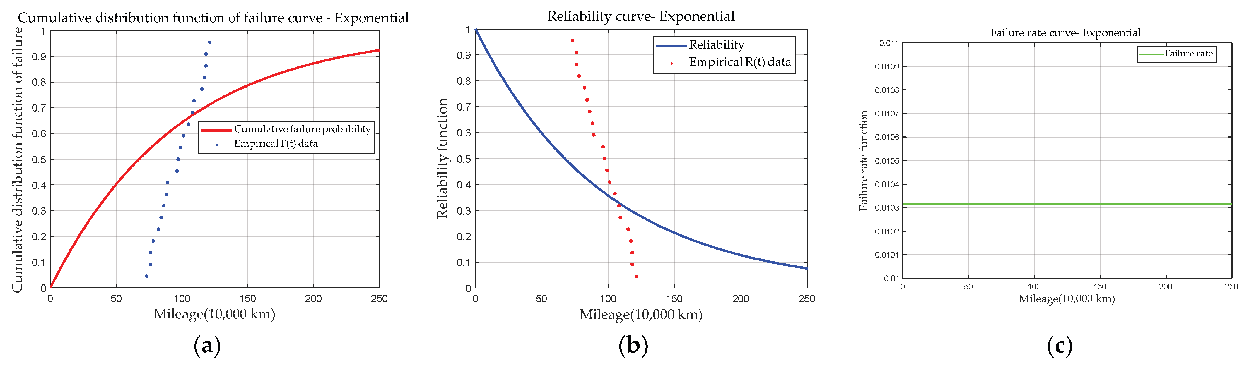
3.2.3. Exponential Distribution

The expression for the failure probability density f ( t ) is as follows:
f ( t ) = λ e λ t
where λ represents the core parameter describing the failure rate, which determines the distribution shape of the exponential distribution’s probability density curve.
The expression for the failure distribution curve F ( t ) is as follows:
F ( t ) = 1 e λ t
The expression for the reliability R ( t ) is as follows:
R ( t ) = e λ t
The expression for the failure rate λ ( t ) is as follows:
λ ( t ) = f ( t ) R ( t ) = λ
The failure rate λ of the exponential distribution is a constant, indicating that the probability of a device failing within a future time period is independent of how long it has already been in operation, thus exhibiting the “memoryless” property.

3.2.4. Two-Parameter Weibull Distribution

The expression for the failure probability density f ( t ) is as follows:
f ( t ) = m η ( t η ) m 1 e ( t η ) m
where m is the shape parameter, which determines the monotonicity of the Weibull distribution’s probability density curve f ( t ) , and η is the scale parameter, which is determined by the equipment’s service environment.
The expression for the failure distribution curve F ( t ) is as follows:
F ( t ) = 1 e ( t η ) m
The expression for the reliability R ( t ) is as follows:
R ( t ) = e ( t η ) m
The expression for the failure rate λ ( t ) is as follows:
λ ( t ) = f ( t ) R ( t ) = m η ( t η ) m 1

3.2.5. Gamma Distribution

The expression for the failure probability density f ( t ) is as follows:
f ( t ) = λ k 0 + x k 1 e x d x t k 1 e λ t
where k is the shape parameter and λ is the scale parameter.
The expression for the failure distribution curve F ( t ) is as follows:
F ( t ) = 1 0 + x k 1 e x d x 0 λ t x k 1 e x d x
The expression for the reliability R ( t ) is as follows:
R ( t ) = 1 0 + x k 1 e x d x λ t + x k 1 e x d x
The expression for the failure rate λ ( t ) is as follows:
λ ( t ) = f ( t ) R ( t ) = t k 1 e λ t λ t + x k 1 e x d x

3.3. The Evaluation Criterion for the Optimal Failure Distribution Curve

The failure times of different types of equipment vary significantly due to differences in material selection, design, manufacturing processes, operational conditions, and service mechanisms. Consequently, different types of failure distribution curves are applicable to different scenarios.
In 1974, the Japanese statistician Hirotugu Akaike proposed a statistical criterion for model selection known as the Akaike Information Criterion (AIC). AIC takes into account both the goodness of fit and the complexity of the model. A model is considered superior if it achieves a better fit with lower complexity. AIC is selected as the evaluation standard for the optimal failure distribution curve to identify the optimal failure distribution model from five commonly used failure distribution curves that best fit the failure patterns of the equipment.
AIC not only measures the model’s fitting performance but also considers its complexity by introducing a penalty term to avoid overfitting. It is defined as follows:
A I C = 2 k ln L
where k represents the number of parameters in the failure distribution curve, indicating the complexity of the model, and L represents the maximum likelihood function, reflecting the goodness of fit. According to the definition, the smaller k and the larger L , the smaller the AIC value, indicating that the distribution curve better characterizes the failure patterns of the equipment and is the optimal failure distribution curve.

3.4. The Health Correction Function Based on the Reliability Indicator

With the increase in service mileage, the component’s failure probability increases monotonically, following the rule of the component’s performance degradation. The greater the component’s unreliability at the current mileage, the greater the failure probability. Therefore, on the basis of the calculated initial health H S of the rolling bearing, the bearing health is dynamically corrected based on the cumulative failure probability F ( t ) . The health correction function is defined as follows:
H S c = H S × e F ( t )

4. Experimental Results and Analysis

4.1. Modeling of Initial Health Assessment Model Based on MSET

4.1.1. Brief Description of Case Western Reserve University Bearing Data Set

The validity of the health assessment method proposed in this paper is verified by using the bearing dataset from the Case Western Reserve University in the United States [30]. The vibration test bench of Case Western Reserve University mainly consists of a 1.5 kW motor, a torque sensor/decoder, a power tester, and an electronic controller. The object to be tested is the motor bearing, which is divided into the drive end bearing and the fan end bearing. In this paper, the rolling bearing at the drive end is selected as the object for health assessment. The sampling frequency is 12 kHz, and the sampling duration for each working condition is about 10 s. Each working condition sample contains 120,000 data points. The fault location is the outer ring of the bearing, and the fault type is a single-point damage caused by an electric spark. The normal base vibration acceleration data operating at four speeds are input into MSET to construct the historical memory matrix to characterize the normal operating state of the bearing. The specific fault severity is shown in Table 1, and the speed conditions of the bearing operation are shown in Table 2.
Based on the fault degree and speed condition of the driving end rolling bearing, 12 kinds of vibration acceleration fault data can be obtained. Under each working condition, 120,000 data points are rounded up, and the vibration acceleration peak, kurtosis, and root mean square (RMS) values are computed for every 2000-sample segment of the acquired data. The steps of data application are as follows: Firstly, the peak value, kurtosis and root-mean-square (RMS) values of normal base data under four speed conditions are extracted to form an observation vector, input into MSET to build the memory matrix, and then the fault data are divided into three groups for verification according to the algorithm verification requirements, which are as follows: data with different fault degrees at the same speed, data in the same fault degree at different speeds, and data with different fault degrees at different speeds.

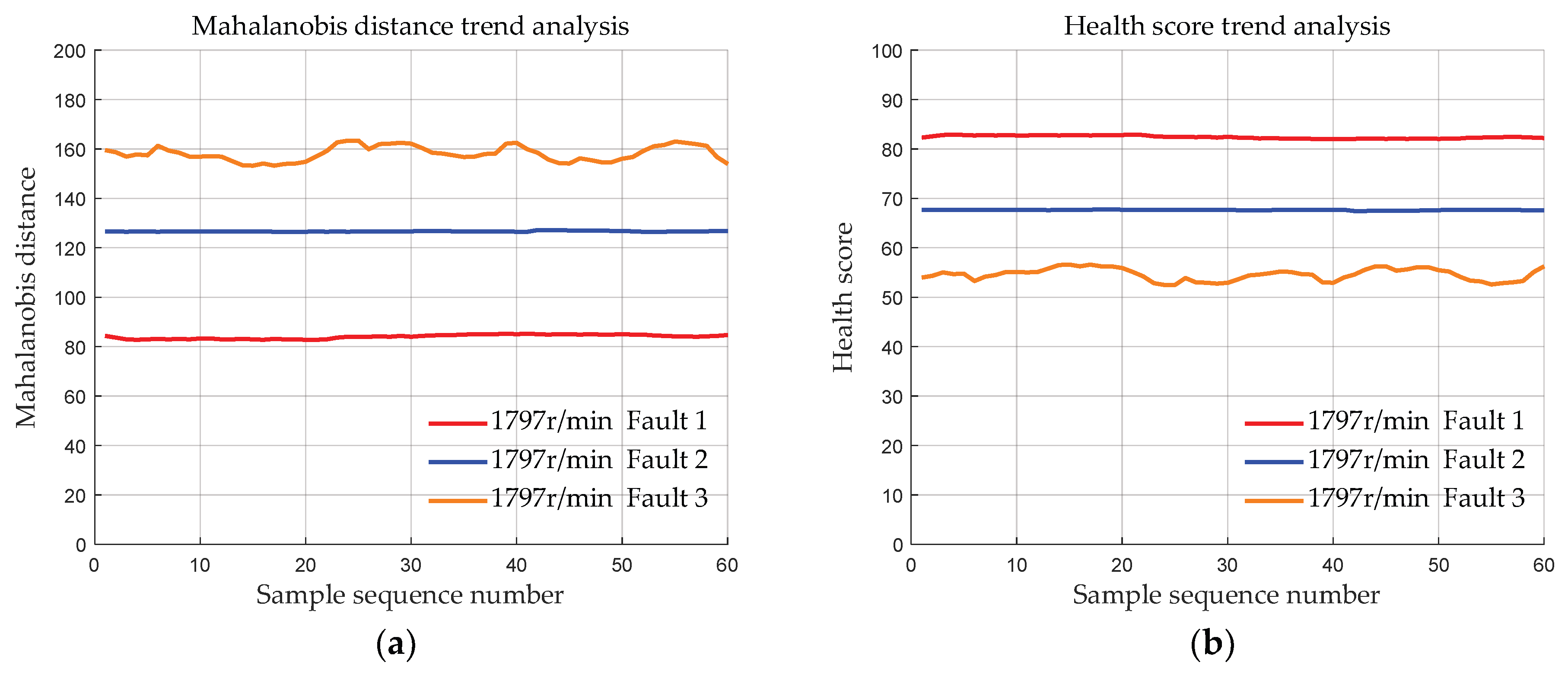
4.1.2. Data with Different Fault Degrees at the Same Speed

The fault rolling bearing data are divided into 4 groups: 1730 r/min, 1750 r/min, 1772 r/min, and 1797 r/min, according to the operating conditions. Each group contains data with 3 fault degrees. The deviation of data with three fault degrees from the health baseline is quantified for each group. The results are shown in Figure 2, Figure 3, Figure 4 and Figure 5.
Figure 2, Figure 3, Figure 4 and Figure 5 show that on the same speed condition, the calculated deviation distance is positively correlated with the fault degree: the greater the fault degree, the greater the corresponding deviation distance, which verifies that the deviation distance of the output of the health assessment model can monotonically represent the fault degree.

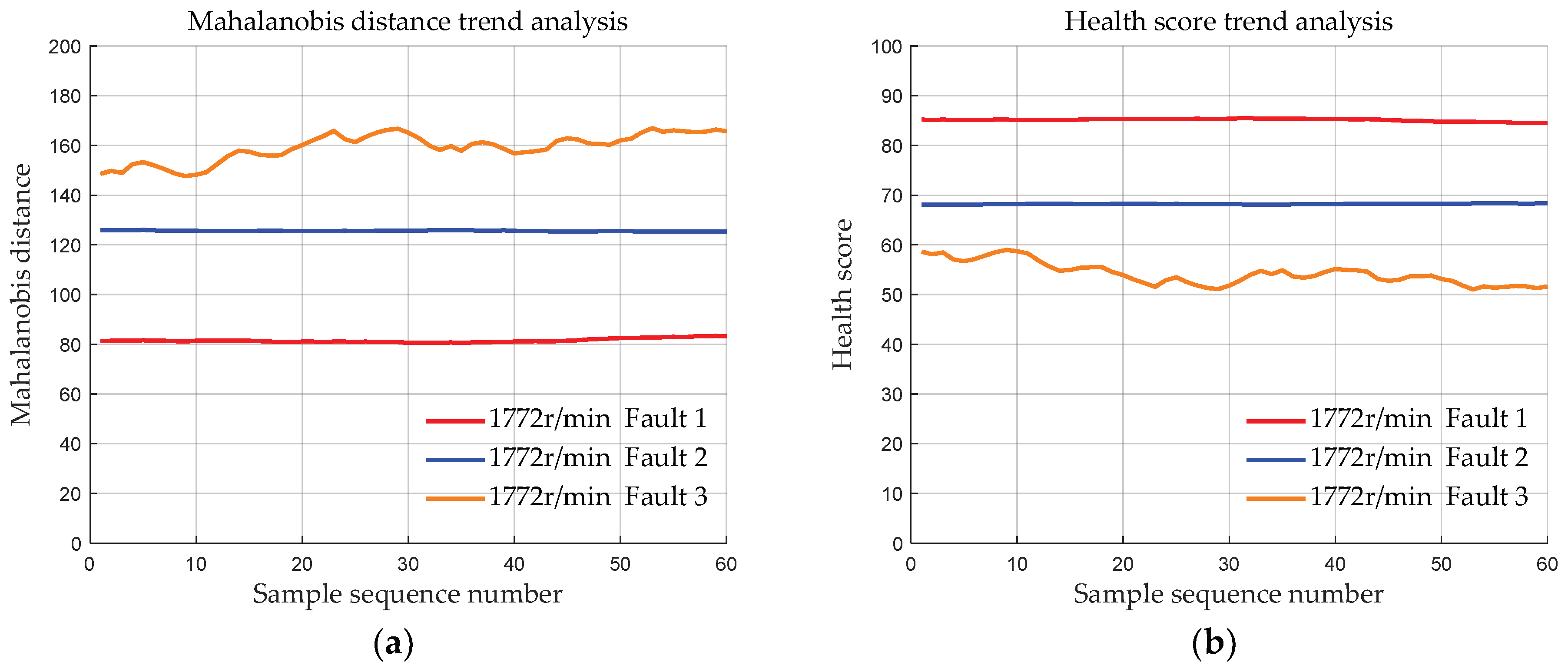
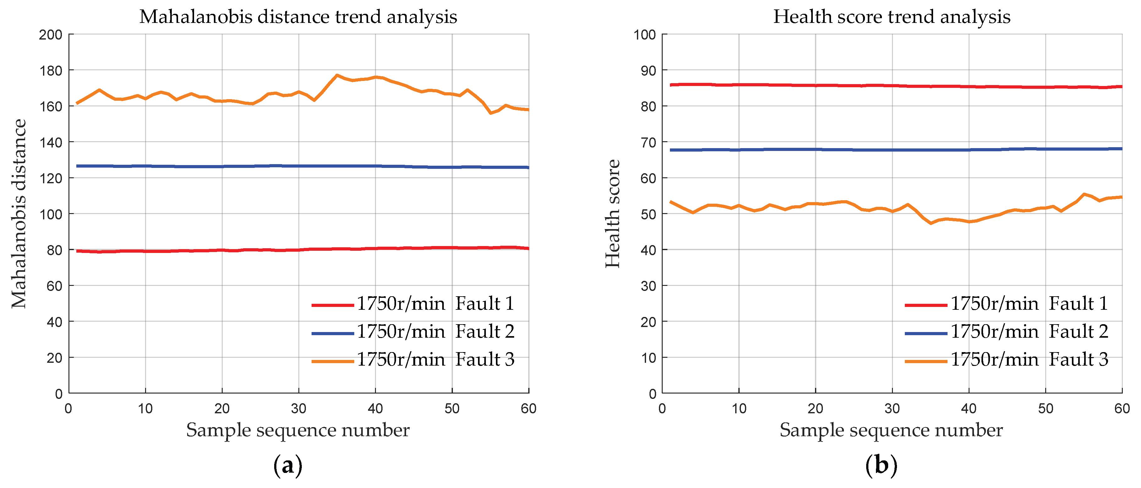
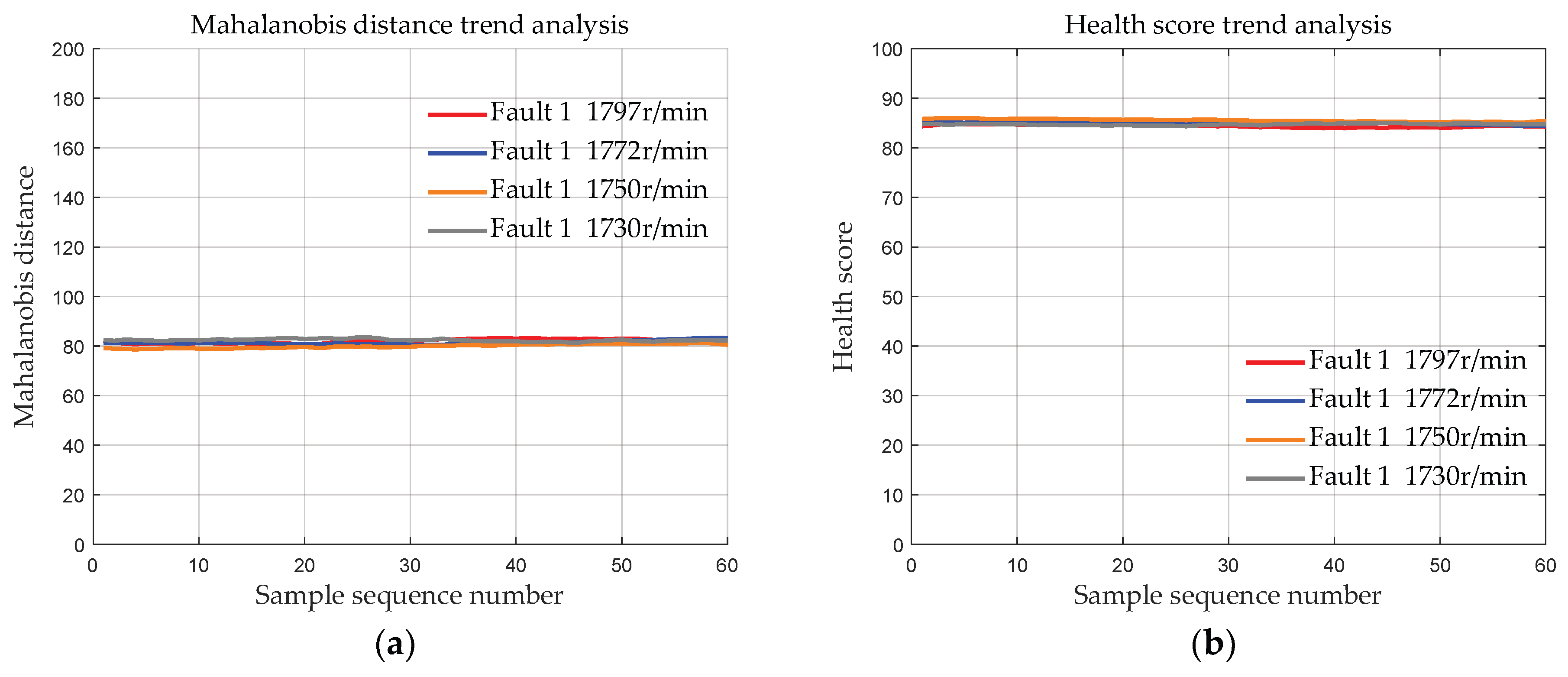
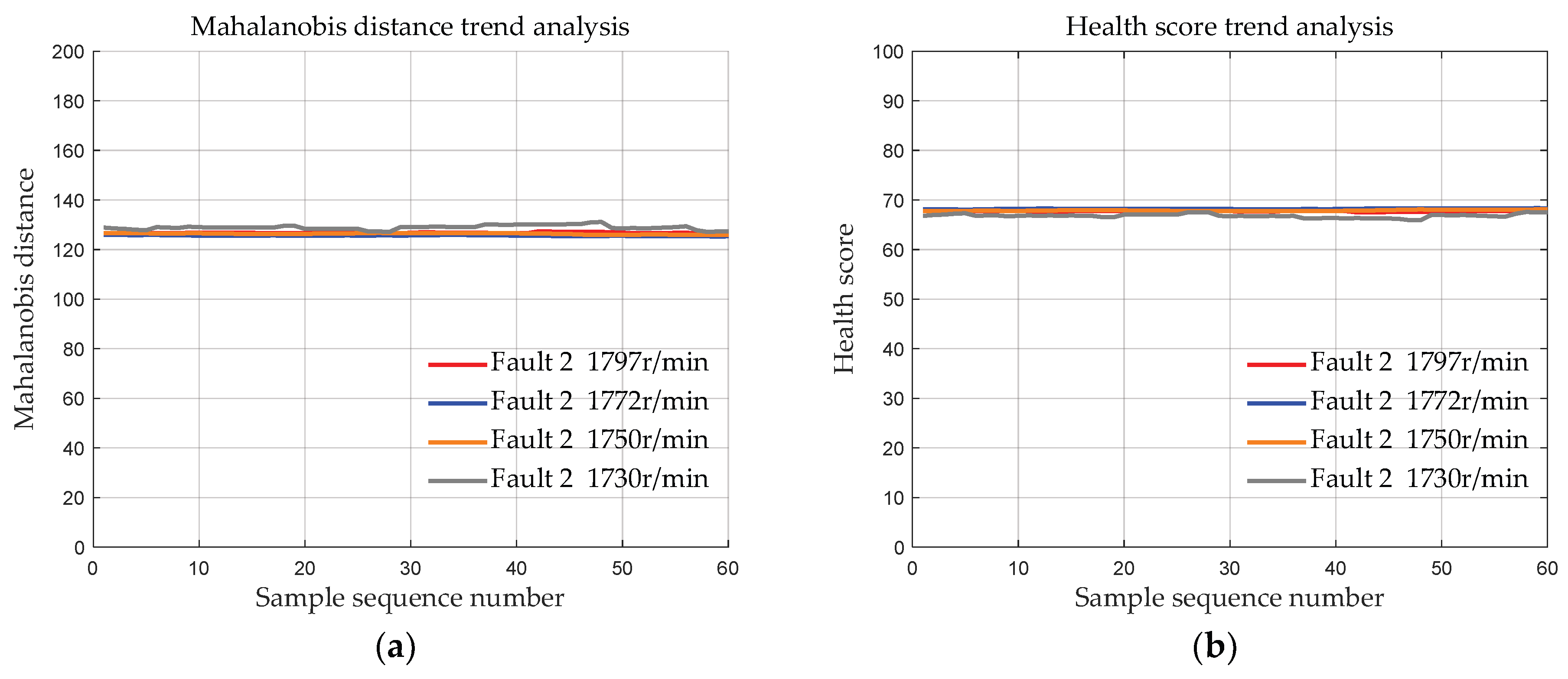
4.1.3. Data with the Same Fault Degree at Different Speeds

Input data with fault 1 and data with fault 2 under four speed conditions into the health assessment model, and the output deviation distance and the evaluated health score are shown in Figure 6 and Figure 7:
Figure 6 shows that the calculated deviation distance of data with fault 1 under four operating speeds of 1730 r/min, 1750 r/min, 1772 r/min and 1797 r/min is concentrated around 80, based on which the health score calculated is 86. Figure 7 shows that the calculated deviation distance of fault 2 under four operating speeds of 1730 r/min, 1750 r/min, 1772 r/min and 1797 r/min is concentrated around 126, based on which the health score calculated is 67. The data of the same fault evaluation remain consistent under different speed conditions. It is verified that the deviation distance calculated by the health assessment model is little affected by the velocity condition, and MSET can reduce the influence of the speed condition.

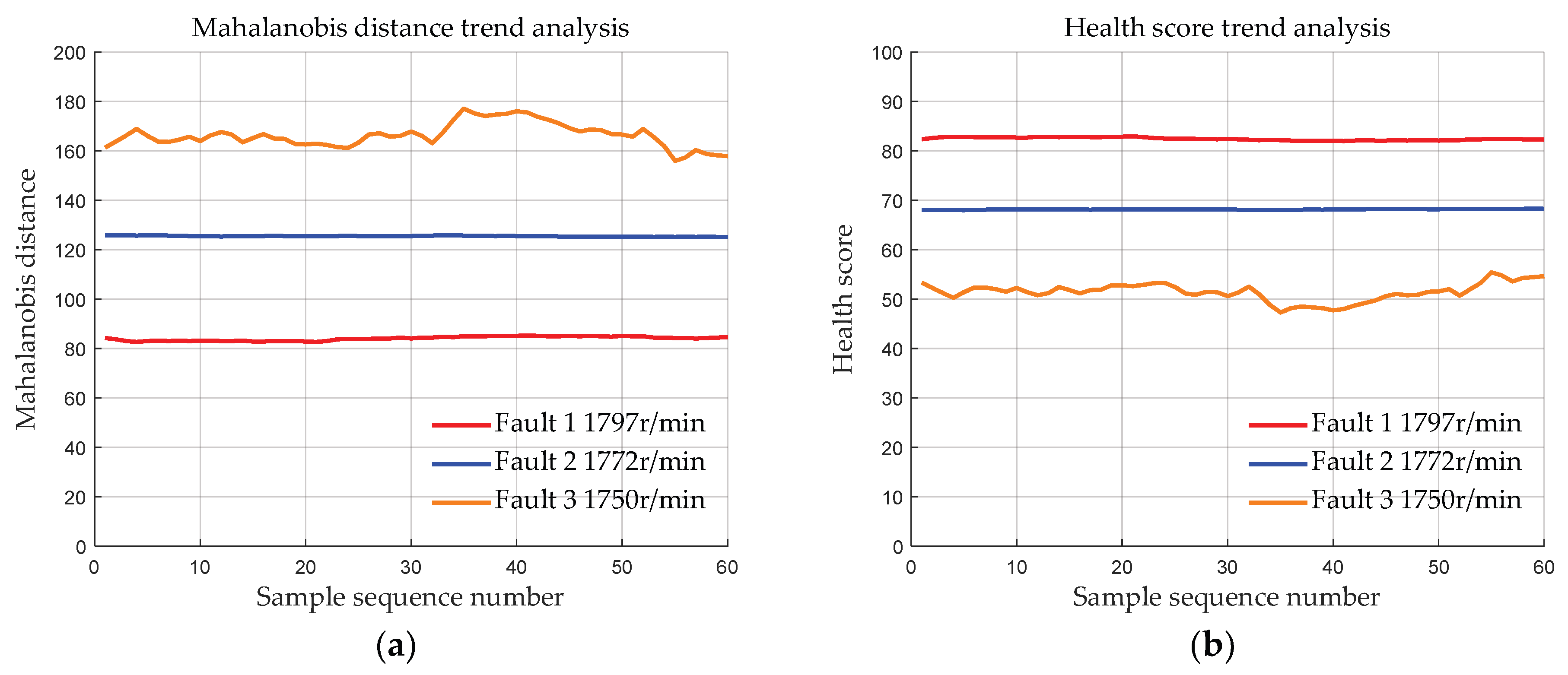
4.1.4. Data with Different Fault Degrees at Different Speeds

Input data with fault 1 at the speed of 1797 r/min, data with fault 2 at the speed of 1772 r/min, and data with fault 3 at the speed of 1750 r/min into the health assessment model, and the output deviation distance is shown in Figure 8.
Figure 8 shows that among the three types of fault data, data with fault has a fault diameter of 0.1778 mm, which is the smallest fault degree, and operates at the speed of 1797 rpm, which is the highest speed condition. It exhibits the smallest deviation distance. On the other hand, data with fault 3 has a fault diameter of 0.5334 mm, which is the largest fault degree, and operates at the speed of 1750 rpm, which is the lowest speed condition. It shows the largest deviation distance. When both the fault degree and the speed change, the deviation distance is primarily determined by the fault degree, thereby reducing the influence of the operating conditions. This verifies that MSET can establish a health baseline that adapts to changes in the operating conditions of the data being evaluated, minimizing the impact of operating conditions on health assessment.

4.2. Health Score Correction Based on the Reliability Model

The establishment of the reliability model for rolling bearings necessitates the collection of historical failure statistics pertaining to identical bearing types operating under equivalent service route conditions. These historical failure data are instrumental in elucidating the performance degradation characteristics of rolling bearings.
Collect historical failure mileage data of rolling bearings in the train bogie and calculate empirical cumulative distribution function value based on Equation (48). The calculated data are shown in Table 3.
F n ( x i ) = i n + 1
where x i refers to the i -th failure mileage data point in ascending order. i refers to the rank of x i . n refers to the total number of collected data.
Based on MATLAB(R2018a), five commonly used failure distribution curves are utilized to fit the empirical data of rolling bearings. The parameters of each failure distribution are calculated using the maximum likelihood estimation method (MLE). The results are as follows:
With AIC serving as the criterion, select the optimal failure distribution model that best characterizes the rolling bearing performance degradation trend. The AIC values of the five failure distribution models are shown in Table 4.
The smaller the AIC value, the better the overall fitting performance. Table 4 indicates that gamma distribution is the optimal fitting model for the current failure data. The exponential function, having only one parameter, exhibits the poorest fitting performance for the current data. As can be intuitively observed from Figure 9, Figure 10, Figure 11, Figure 12 and Figure 13, its fitting effect significantly differs from that of the other four failure distribution models.
Then, the rolling bearing’s initial health score is corrected based on the gamma distribution. Assuming the current initial health score of the rolling bearing in the bogie of the in-service train is 100, the corrected health scores at 500,000 km, 600,000 km, 700,000 km, 800,000 km and 900,000 km are calculated, as shown in Table 5.
Table 5 shows that as the service mileage increases, the performance of the rolling bearing gradually degrades, and its corrected health score progressively declines, which is consistent with the actual performance state of the bearing.

5. Conclusions

This study addresses the challenges in assessing the health status of in-service rolling bearings for trains, which are often affected by operating conditions, leading to frequent false alarms and missed detections. Additionally, the impact of service mileage on bearing performance degradation is often overlooked, resulting in incomplete and inaccurate health assessments. To tackle these issues, a novel health assessment methodology based on MSET and reliability analysis is proposed. Initially, the bearing’s initial health score is evaluated using MSET. This involves selecting three strongly correlated feature indicators from the bearing’s vibration acceleration to form an observation vector. Subsequently, a health-data space under multiple operating conditions is established using MSET. The deviation distance is quantified using Mahalanobis distance, and the initial health score of the bearing is derived by integrating a health mapping function. Furthermore, the initial health score is corrected using the reliability model that incorporates service mileage as a critical factor in the health assessment. This approach leverages multi-source data to provide a comprehensive, multidimensional health assessment of bearings, offering essential theoretical guidance for bearing maintenance. The main conclusions are as follows:
(1)
Validation was conducted using the bearing dataset from Case Western Reserve University to demonstrate the effectiveness of the initial bearing evaluation model based on MSET. The results show that the deviation distances of the bearing data of the three fault degrees calculated by the proposed method are approximately 83, 127, and 170, respectively. Moreover, the deviation distances of the bearings of each fault degree are basically the same at 4 different speeds, indicating that MSET can reduce the influence of the speed conditions on the bearing health assessment, ensuring that the health score is primarily determined by the fault severity.
(2)
Considering the natural performance degradation of bearings over service mileage, the reliability model was introduced to correct the initial health assessment of the bearings. Based on historical failure data and using AIC as the evaluation standard, the fitting performance of five commonly used failure distribution models was compared. With the Gamma distribution providing the smallest AIC value (178.592) among candidate distributions, the Gamma distribution was the best fit. As the service mileage increases, the corrected health score of the bearing gradually declines from 99.9 to 70.97, indicating the performance degradation of the bearing.

Author Contributions

Conceptualization, C.C.; methodology, C.C. and L.L.; software, L.L.; validation, L.L.; formal analysis, C.C.; resources, L.L. and C.C.; writing—original draft preparation, C.C. and L.L.; writing—review and editing, C.C.; supervision, C.C. All authors have read and agreed to the published version of the manuscript.

Funding

This research was funded by the National Natural Science Foundation of China (No. 52372402) and the National Natural Science Foundation of China (No. 51975487).

Data Availability Statement

The original contributions presented in the study are included in the article; further inquiries can be directed to the corresponding author.

Conflicts of Interest

The authors declare no conflicts of interest.

Nomenclature

x r m s Root mean square acceleration, in g.
x p Peak acceleration, in g.
KKurtosis of acceleration.
X ( t j ) Time-series of feature indicators for the component at tj.
X o b s The observation vector.
DThe memory matrix.
X e s t The estimation vector.
WThe weight vector.
εThe residue between the observation vector and the estimation vector.
The nonlinear operator.
F ( t ) Cumulative failure probability.
f ( t ) Failure probability density.
R ( t ) Reliability.
λ ( t ) Failure rate.

References

  1. He, M.; Guo, W. An integrated approach for bearing health indicator and stage division using improved Gaussian mixture model and confidence value. IEEE Trans. Ind. Inform. 2021, 18, 5219–5230. [Google Scholar] [CrossRef]
  2. Braun, S. The extraction of periodic waveforms by time domain averaging. Acustica 1975, 32, 69–77. [Google Scholar]
  3. Chaturvedi, G.K.; Thomas, D.W. Bearing fault detection using adaptive noise canceling. J. Sound Vib. 1982, 104, 280–289. [Google Scholar]
  4. Tan, J.Y.; Chen, X.F.; He, Z.J. Adaptive detection method of random resonance for impulse signals. J. Mech. Eng. 2010, 46, 61–67. [Google Scholar] [CrossRef]
  5. Yao, D.C. Fault Diagnosis Technology of Rail Transit Bearing; China Railway Publishing House: Beijing, China, 2017; pp. 45–47. ISBN 978-7-113-22353-3. [Google Scholar]
  6. Tang, D.Y. Generalized Resonance, Resonance Demodulation Fault Diagnosis and Safety Engineering Urban Rail Traffic; China Railway Publishing House: Beijing, China, 2013; pp. 17–18. ISBN 978-7-113-17412-5. [Google Scholar]
  7. Noman, K.; Li, Y.; Peng, Z.; Wang, S. Continuous health monitoring of bearing by oscillatory sparsity indices under non stationary time varying speed condition. IEEE Sens. J. 2022, 22, 4452–4462. [Google Scholar] [CrossRef]
  8. Zhang, B.; Zhang, S.; Li, W. Bearing performance degradation assessment using long short-term memory recurrent network. Comput. Ind. 2019, 106, 14–29. [Google Scholar] [CrossRef]
  9. Shao, X.; Kang, X.W.; Cao, X.R.; Wang, X.P.; Yuan, X.J.; Sun, L. Research on Gearbox Health Assessment Method Based on SOM Neural Network. J. Ord. Equip. Eng. 2021, 7, 246–251. [Google Scholar]
  10. Qifeng, Y.; Longsheng, C.; Naeem, M.T. Hidden Markov Models based intelligent health assessment and fault diagnosis of rolling element bearings. PLoS ONE 2024, 19, e0297513. [Google Scholar] [CrossRef] [PubMed]
  11. Zhang, L.; Huang, W.Y.; Xiong, G.L.; Cao, Q.S. Assessment of Rolling Bearing Performance Degradation Using Gauss Mixture Model and Multi-domain Features. China Mech. Eng. 2014, 22, 3066–3072. [Google Scholar]
  12. Gao, T.; Li, Y.; Huang, X.; Wang, C. Data-driven method for predicting remaining useful life of bearing based on Bayesian theory. Sensors 2020, 21, 182. [Google Scholar] [CrossRef]
  13. Zhang, L.; Wu, R.Z.; Zhou, J.M.; Yi, J.Y.; Xu, T.P.; Wang, L.; Zou, M. Time Series multivariate State Estimation Method of Rolling Bearing Performance Degradation. Vib. Test Diagn. 2021, 6, 1096–1104+1235–1236. [Google Scholar] [CrossRef]
  14. Yu, J.M.; Zhai, X.F.; Wei, S.Y.; Zhao, Q.B.; Cai, Y.B. Early Fault Monitoring Method of Rotating Equipment Based on Multivariate State Estimation. J. Autom. Appl. 2022, 8, 42–45. [Google Scholar] [CrossRef]
  15. Zou, H.B.; Zhang, X.Y.; Li, Q.L. Turbine Fault Warning Algorithm Based on Association Rules and Multiple State Estimation. J. Jilin Univ. 2024, 11, 3283–3288. [Google Scholar]
  16. Wang, Z.; Liu, C. Wind turbine condition monitoring based on a novel multivariate state estimation technique. Measurement 2021, 168, 108388. [Google Scholar] [CrossRef]
  17. Zeng, Y.; Zhang, Y.; Yan, X.; Miao, Q. EMA health indicator extraction based on improved multivariate state estimation technique with a composite operator. IEEE Sens. J. 2023, 23, 19894–19904. [Google Scholar] [CrossRef]
  18. Fan, T.; Tian, S.; Hu, Z.; Fan, X.; Wang, S. Correlation-aware sport training evaluation for players with trust based on Mahalanobis distance. IEEE Access 2021, 10, 16898–16905. [Google Scholar] [CrossRef]
  19. Sun, B.Y. Research on Fault Early Warning Method of Induced Draft Fan Based on Multivariate State Estimation. Master’s Thesis, North China Electric Power University, Beijing, China, 2021. [Google Scholar] [CrossRef]
  20. Tu, W.B.; Liang, J.; Zhou, J.M.; Yang, J.W.; Yang, B.M. Sensitivity Analysis of Rolling Bearing Vibration Characteristic Evaluation Index. Noise Vib. Control 2022, 4, 93–99+131. [Google Scholar] [CrossRef]
  21. Sun, J.Z. Research on Unit Oriented Aero Engine Health State Evaluation and Prediction Method. Ph.D. Thesis, Nanjing University of Aeronautics and Astronautics, Nanjing, China, 2012. [Google Scholar]
  22. Yu, X.G.; Wang, L.C.; Zeng, J.; Wei, X.; Qiu, B.B. Failure early warning and positioning method based on dynamic memory matrix and weighted multivariate state estimation. Ther. Power Gen. 2025, 3, 140–149. [Google Scholar] [CrossRef]
  23. Song, Y.; Zhang, Z.L. Steam Turbine Condition Monitoring Based on Multivariate State Estimation Technique and Hyper-ellipsoid Analysis. J. Chin. Soc. Power Eng. 2020, 2, 138–144. [Google Scholar] [CrossRef]
  24. Wu, T.; Wang, Y.; Liu, Z.; Luo, R.; Liu, F.; Li, Y.; Li, M.; Shi, L. Coal mill fault warning based on multi-state estimation-analytic hierarchy process. Ther. Power Gen. 2023, 5, 14–21. [Google Scholar] [CrossRef]
  25. Cao, S.; Qiu, C.; Ding, C.; Wang, Y. Application of Multiple State Estimation Model Based on Improved entropy weight Method in Turbine energy efficiency Monitoring. J Ther. Energy Power Eng. 2023, 7, 185–193. [Google Scholar] [CrossRef]
  26. Duan, D.; Han, S.; Wang, Z.; Pang, C.; Yao, L.; Liu, W.; Yang, J.; Zheng, C.; Gao, X. Multivariate state estimation-based condition monitoring of slurry circulating pumps for wet flue gas desulfurization of power plants. Eng. Fail. Anal. 2024, 159, 108099. [Google Scholar] [CrossRef]
  27. Wu, Z.Y.; Sun, B. Life Evaluation of digital-analog Linkage Rolling Bearing Based on Mahalanobis Distance. J. Autom. Appl. 2024, 8, 207–210. [Google Scholar] [CrossRef]
  28. Ma, X.B. Reliability Statistical Analysis; Beijing Aerospace University Press: Beijing, China, 2020; pp. 1–5. ISBN 978-7-5124-3217-8. [Google Scholar]
  29. Cheng, J.W.; Liu, X.G.; Dong, H.G.; Zhu, Z.X. Model of Vehicle Failure Rate. J. Mil. Transp. 2015, 1, 38–42. [Google Scholar] [CrossRef]
  30. Smith, W.A.; Randall, R.B. Rolling element bearing diagnostics using the Case Western Reserve University data: A benchmark study. Mech. Syst. Signal Process. 2015, 64–65, 100–131. [Google Scholar] [CrossRef]
Figure 1. Flowchart of health score correction based on the reliability model.
Applsci 15 05396 g001
Figure 2. (a) Deviation distance of 3 kinds of faults at 1797 r/min; (b) Health score of 3 kinds of faults at 1797 r/min.
Applsci 15 05396 g002
Figure 3. (a) Deviation distance of 3 kinds of faults at 1772 r/min; (b) Health score of 3 kinds of faults at 1772 r/min.
Applsci 15 05396 g003
Figure 4. (a) Deviation distance of 3 kinds of faults at 1750 r/min; (b) Health score of 3 kinds of faults at 1750 r/min.
Applsci 15 05396 g004
Figure 5. (a) Deviation distance of 3 kinds of faults at 1730 r/min; (b) Health score of 3 kinds of faults at 1730 r/min.
Applsci 15 05396 g005
Figure 6. (a) Deviation distance of data with fault 1 at different speeds; (b) Health score of data with fault 1 at different speeds.
Applsci 15 05396 g006
Figure 7. (a) Deviation distance of data with fault 2 at different speeds; (b) Health score of data with fault 2 at different speeds.
Applsci 15 05396 g007
Figure 8. (a) Deviation distance of data with different faults at different speeds; (b) Health score of data with different faults at different speeds.
Applsci 15 05396 g008
Figure 9. (a) Normal model fitting to estimated values of cumulative failure probability; (b) Normal model fitting to estimated values of reliability; (c) Normal model fitting to estimated values of failure rate.
Applsci 15 05396 g009
Figure 10. (a) Log-normal model fitting to estimated values of cumulative failure probability; (b) Log-normal model fitting to estimated values of reliability; (c) Log-normal model fitting to estimated values of failure rate.
Applsci 15 05396 g010
Figure 11. (a) Exponential model fitting to estimated values of cumulative failure probability; (b) Exponential model fitting to estimated values of reliability; (c) Exponential model fitting to estimated values of failure rate.
Applsci 15 05396 g011
Figure 12. (a) Two-parameter weibull model fitting to estimated values of cumulative failure probability; (b) Two-parameter weibull model fitting to estimated values of reliability; (c) Two-parameter weibull model fitting to estimated values of failure rate.
Applsci 15 05396 g012
Figure 13. (a) Gamma model fitting to estimated values of cumulative failure probability; (b) Gamma model fitting to estimated values of reliability; (c) Gamma model fitting to estimated values of failure rate.
Applsci 15 05396 g013
Table 1. Fault degree of the driving end rolling bearing.
Fault DegreeFault 1Fault 2Fault 3
Fault diameter (mm)0.17780.35560.5334
Table 2. The speed conditions of the rolling bearing operation.
Motor Load0123
Approximate motor speed (r/min)1797177217501730
Table 3. The data set of the rolling bearing.
No.Mileage (10,000 km)Empirical Cumulative Distribution Function ValueEmpirical Reliability Function Value
1730.04550.9545
2760.09090.9091
3760.13640.8636
4780.18180.8182
5820.22730.7727
6840.27270.7273
7860.31820.6818
8880.36360.6364
9890.40910.5909
10960.45450.5455
11970.50000.5
12990.54550.4545
131010.59090.4091
141050.63640.3636
151080.68180.3182
161090.72730.2727
171150.77270.2273
181170.81820.1818
191180.86360.1364
201180.90910.0909
211210.95450.0455
Table 4. AIC values of 5 failure distribution models.
Failure Distribution ModelNormalLog-NormalExponentialWeibullGamma
AIC value178.5920178.6018236.1172178.7564178.4728
Table 5. The corrected health scores of the rolling bearing at several service mileages are based on the gamma distribution.
Service Mileage500,000 km600,000 km700,000 km800,000 km900,000 km
Corrected health score99.999.6796.9987.4670.97
Disclaimer/Publisher’s Note: The statements, opinions and data contained in all publications are solely those of the individual author(s) and contributor(s) and not of MDPI and/or the editor(s). MDPI and/or the editor(s) disclaim responsibility for any injury to people or property resulting from any ideas, methods, instructions or products referred to in the content.

