Feature Fusion Graph Consecutive-Attention Network for Skeleton-Based Tennis Action Recognition

Abstract

Human action recognition has become a key direction in computer vision. Deep learning models, particularly when combined with sensor data fusion, can significantly enhance various applications by learning complex patterns and relationships from diverse data streams. Thus, this study proposes a new model, the Feature Fusion Graph Consecutive-Attention Network (FFGCAN), in order to enhance performance in the classification of the main tennis strokes: forehand, backhand, volley forehand, and volley backhand. The proposed network incorporates seven basic blocks that are combined with two types of module: an Adaptive Consecutive Attention Module, and Graph Self-Attention module. They are employed to extract joint information at different scales from the motion capture data. Due to focusing on relevant components, the model enriches the network’s comprehension of tennis motion data representation and allows for a more invested representation. Moreover, the FFGCAN utilizes a fusion of motion capture data that generates a channel-specific topology map for each output channel, reflecting how joints are connected when the tennis player is moving. The proposed solution was verified utilizing three well-known motion capture datasets, THETIS, Tennis-Mocap, and 3DTennisDS, each containing tennis movements in various formats. A series of experiments were performed, including data division into training (70%), validating (15%), and testing (15%) subsets. The testing utilized five trials. The FFCGAN model obtained very high results for accuracy, precision, recall, and F1-score, outperforming the commonly applied networks for action recognition, such as the Spatial-Temporal Graph Convolutional Network or its modifications. The proposed model demonstrated excellent tennis movement prediction ability.

1. Introduction

Human Action Recognition (HAR) is currently widely applied to recognize complex movements of athletes, including accuracy prediction or to detect objects in images or videos [1]. Due to the large amount of data gathered via YouTube, traffic cameras, social media, and motion capture systems, as well as stored in publicly available datasets, this area of Computer Vision (CV) possesses sufficient sources to apply deep learning (DL) models in order to enhance athlete’s performance. These modern techniques may also encourage people to learn and master sports skills. Recognition of sports movements plays a pivotal role in monitoring athletes during training, matches, and competitions. Another aspect of HAR is to verify how sport movements are performed. For these tasks, the recognition of specific moves is essential. The development of vision systems allows one to obtain increasingly accurate data, which in the case of sport analysis is of a very significant importance.

The main challenges of HAR are faced in detecting sport actions and activities, which are further applied for monitoring a player’s performance. Recently studies have focused on fusion of the skeleton structure of sensor-based data, together with other representations like joint position and velocities [2], kinematics data [3], and trajectories [4,5,6,7]. These approaches provide topological relations that are further utilized in the recognition process. The fusion of motion capture data provides a better representation of this kind of data. Thus, this study focuses on discussing the fundamental issues of high-accuracy tennis movement recognition. DL models have difficulties in accurately identifying both short-term and long-term dynamic characteristics, as well as in extracting joint information at different scales from motion capture data, especially for very dynamic movements. In response to the above challenges, the authors proposed a new model for recognizing the main tennis movements. The main contributions are as follows:

• Motion capture datasets containing basic tennis strokes were selected, such as THETIS, Tennis-Mocap, and 3DTennisDS. The first contains data recorded with a markerless system, while the latter two used optical, retro-reflective systems. The data contain the positions of participants performing individual tennis movements. The 3DTennisDS dataset additionally contains the position of the tennis racket.
• Participant data obtained from the three datasets were unified and simplified to the THETIS dataset, in order to create similar input data for the model.
• The following tennis movements were chosen to recognize: forehand, backhand, volley forehand, and volley backhand.
• The authors propose a new model to recognize the abovementioned tennis moves. The Feature Fusion Graph Consecutive-Attention Network (FFGCAN) was created, which incorporates seven basic blocks that are combined with two types of module: Adaptive Consecutive Attention Module, and Graph Self-Attention. Additionally, a temporal convolutional network, as a part of the network, models short-term temporal dependencies.
• The FFGCAN was verified utilizing the following metrics: accuracy, precision, recall, F1-score, and confusion matrices. The training process toward accurate prediction was analyzed.
• In order to visualize which features are the most essential for tennis movement recognition, Gradient-weighted Class Activation Mapping (Grad-CAM) was applied. This CV technique indicated the most relevant data for making predictions.

2. Related Works

Tennis stroke recognition has been of great interest recently. Many studies concerning tennis movement detection are performed, utilizing various types of data, such as motion capture, images, video, and sensors. For these purposes, publicly available datasets are applied, as well as data captured by the authors. Many Machine Learning and Deep Learning models have been proposed for tennis stroke recognition.

Motion capture data of movements have been obtained for various systems, including markerless and marker-based. The THETIS dataset was created utilizing the Microsoft Kinect system. It contains twelve tennis moves, such as forehand, backhand, volley, service, and smash, as well as their types. A great number of studies concerning tennis stroke recognition have been performed utilizing this dataset. The five-layer deep historical Long Short-Term Memory (LSTM) network together with the Inception V3 model were combined for classification of tennis moves from video sequences [8]. All captured moves were detected using InceptionResNetV2 and ResNet152V2. The CNN-LSTM network was applied for feature extraction from RGB video and Xception for spatial feature extraction [9]. A 3-layered LSTM model was also proposed to classify these moves. In the studies in [10,11], the Inception network was chosen for feature extraction from RGB videos. The LSTM model with channel and attention modules was also applied for recognition of six tennis moves [12]. Linear-Chain Conditional Random Fields and Support Vector Machine were also used for classification of tennis moves [13]. Distinguishing the level of tennis players, taking into account twelve strokes, was performed utilizing k-NN classification with Dynamic Time Warping (DTW) [14]. Tennis forehand and backhand swing were detected utilizing a time-series CNN based on MPU9250 sensor [15]. A Hilbert-embedding-based framework (EHECCO) was used to extract the nonlinear dependencies for time series classification based on motion capture data, Tennis-Mocap, CMU, and HDM05 [16]. A multimodal solution, the Adaptive Semantic-Enhanced Convolutional Neural Network, was proposed for complex action classification from tennis data using the THETIS and Tennis-Mocap datasets [17]. The model integrates a Large Language Model to obtain an action semantic enhancement mechanism.

Apart from the available datasets, a lot of studies have used data captured for the purpose of the research. Forehand and backhand swing were analyzed utilizing a Hidden Markov Model, where hand positions were indicated [18]. Forehand, backhand, serve, and volley were detected based on inertial sensor data, from the PIQ Robot sports tracker, utilizing Learning Vector Quantization [19]. A Deep Neural Network was applied for serve, backhand, and forehand recognition using tennis racket orientation gathered from a wearable SensorTile [20]. Decision Tree (DT), SVM, Neural Networks (NN), and k-NN methods were applied for classification of six tennis movements [21]. A SVM with a radial basis function kernel and k-NN methods were chosen for tennis serve, forehand, and backhand recognition [22]. The study involved data gathered from an eight-video camera system and IMU sensor.

A series of studies concerning the recognition of forehand, backhand, volley forehand, and volley backhand strokes obtained from motion capture data, registered with tennis players together with a tennis racket, can be found in [23,24,25,26,27]. The movements were performed with and without a tennis ball, which were gathered into the 3DTennisDS dataset [24]. The adjusted Spatial-Temporal Graph Neural Network (ST-GCN) together with active features was applied for images presenting the model of a tennis player holding a tennis racket, and reflecting the silhouette and the tennis racket position for the abovementioned moves [23]. Moreover, the fuzzification of input data with a trapezoidal function improved the classification accuracy. The same model was applied for forehand, backhand, and volley recognition based on data from three datasets, 3DTennisDS, THETIS, and Tennis-Mocap [24]. An Attention Temporal Graph Convolutional Network, involving an attention model defined as an encoder–decoder, and a BiDirectional Recurrent Neural Network for extracting temporal features and Graph Convolutional Networks for calculating spatial features were proposed for recognition of the abovementioned tennis strokes gathered in the 3DTennisDS dataset [25]. Another modification of an Attention Temporal Graph Convolutional Network with Gated Recurrent Unit for extracting temporal attention for classification of forehand and backhand strokes with phases of these moves was described in [26]. A Dual Attention Graph Convolutional Network combining two attention modules, a Graph Convolutional Network for extracting spatial features and LSTM for temporal features, was applied for four tennis strokes based on the 3DTennisDS dataset [27]. All SY-GCN- based models proved to have a high performance.

3. Problem Definition

Tennis stroke classification involves examining continuous time series recordings that illustrate a tennis player’s body movements, in order to classify them into one of the defined stroke categories. The 2D poses of a person with joints over frames can be expressed mathematically as in Equation (1) [28]:

$$P_{obs}^{2D}=[P_1,P_2,\dots ,P_i,\dots ,P_T]\in {\mathbb{R}}^{T\times J\times 2}$$

(1)

Here, each $P_i\in {\mathbb{R}}^{J\times 2}$ corresponds to the 2D coordinates of all J joints at frame i. Given these observed sequences of 2D player poses, the primary goal in tennis motion classification is to develop a parametric model capable of accurately assigning each sequence to one of several predefined action or stroke classes. Formally, this can be represented by (2):

$$\widehat{y}=\mathrm{Model}\left(P_{obs}^{2D}\right)\mathrm{where}\widehat{y}\in \{c_1,c_2,\dots ,c_M\}$$

(2)

where $\widehat{y}$ is the predicted stroke class, and $c_1,c_2,\dots ,c_M$ represents the set of all possible stroke classes. We use spatio-temporal graphs to represent the observed skeleton poses at J joints for one person in T frames. At each frame t, we characterize a spatio-temporal graph $G_t=(V_t,E_t)$. Here, the set of vertices $V_t$ indicates the skeletal joints, and the set of edges $E_t$ shows the connections between these joints. Positional information for each node at time t is stored. The edges are defined using an adjacency matrix $A_t$, where its entries $a_{i,j}=1$ denote connected joints and $a_{i,j}=0$ denote disconnected ones. Thus, the input to the classification model is then represented as ${\left\{G_t^{2D}\right\}}_{t=1}^T$.

4. Preliminaries

Human skeletal data, in terms of skeleton-based action classification, are usually represented in the form of a graph structure $G=(V,E)$. Here, $V\in {\mathbb{R}}^{N\times C}$ denotes a set containing N joint nodes. Each node has C features (for example, spatial coordinates or velocities of joints). The edge set E represents connections between the nodes and can be expressed through an adjacency matrix $A\in {\mathbb{R}}^{N\times N}$. Graph Convolutional Networks (GCNs) have become popular in recent papers because they perform well in modeling problems classifying actions based on skeletons [26,29,30,31]. Usually, a 3D time skeleton sequence used for classification is shown as a tensor $f_{in}\in {\mathbb{R}}^{C\times T\times N}$, where C denotes the channel dimension, T the number of frames, and N the number of nodes of joints. The fundamental relationship for classic GCNs is defined by Equation (3):

$$f_{out}=\sigma \left({\Lambda }^{{\displaystyle \frac{1}{2}}}(A+I){\Lambda }^{{\displaystyle \frac{1}{2}}}{f}_{in}W\right)$$

(3)

Here, ${\Lambda }^{{\displaystyle \frac{1}{2}}}(A+I){\Lambda }^{{\displaystyle \frac{1}{2}}}$ denotes an A matrix using a diagonal $\Lambda$ matrix for normalization. $\sigma$ is any nonlinear activation function like $ReLU$ or sigmoid, and W is a learnable weight matrix that combines features across channels [31,32].

5. Materials and Methods

In the proposed model, feature fusion is described as combining multiple complementary elements of a single skeleton into a richer description. In practice, three feature families are combined: absolute joint coordinates, bone vectors defined as differences between neighboring joints, and motion vectors calculated as differences in position in the subsequent frames. Each of these modalities is first projected through a separate lightweight $1\times 1$ convolution projection to allow encoding patterns specific to each description space without mutual suppression of information. These tensors are subsequently concatenated along the channel dimension normalized with BatchNorm and fed into the subsequent graph-attention blocks.

In this model, feature fusion is described as combining multiple complementary elements of a skeleton into a single, richer description. The model puts out two link lists: a fixed, globally taught one, and a changing one, worked out in each frame using Adaptive Consecutive Attention. Both lists are weighted using the learned values and added together, making a map that shows the present, path-based links between joints. The feature values are then multiplied by their corresponding topological maps, so that the result preserves the time–node alignment. This considers the context of whole-body motion. This scheme allows the network to treat the same pose differently according to the direction and speed of motion.

5.1. Datasets

This study incorporates three datasets containing tennis movements, registered using markerless and marker-based motion capture systems. The data for the study were unified and simplified according to the THETIS dataset, in order to standardize the input data to the model.

5.1.1. THETIS

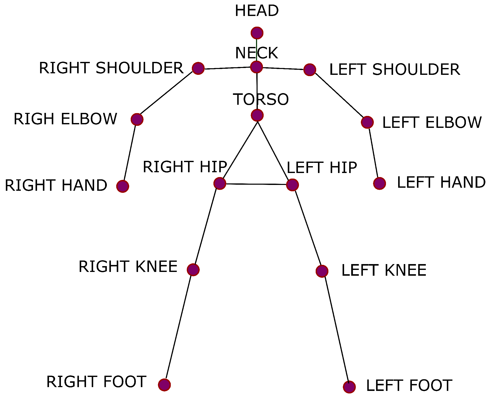
The THETIS (Three dimEnsional TennIs Shot) dataset was created in 2013 [33]. Twelve tennis strokes were registered by Microsoft’s Kinect motion capture system. They were performed by thirty-one amateurs and twenty-four professional tennis players. The data collection included twelve movements: backhand (one-handed, two-handed, slice), volley (backhand and forehand), forehand (flat, open stands, slice), service (flat, kick, slice) and smash. The following data formats are available in the dataset: ONI files, depth and RGB videos, silhouette, skeleton 2D and 3D videos, and skeleton joints. THETIS is a very well-known dataset that has been incorporated in many papers recently. In this study, the authors focus on ONI files that reflect a model of the tennis player. The model involves 15 points (Figure 1).

5.1.2. Tennis-Mocap

The Tennis-Mocap dataset was created in 2020 [16]. It consists of motion capture data of 17 athletes from the Caldas-Colombia tennis league. Five of the participants were stated to be high performers and the others regular performers. Their movements were recorded using an Optitrack Flex V100 including six cameras, with the frequency set to 100 Hz. Thirty-four markers, defined by Arena software, were attached for collecting information about their body joints. The study was performed according to the Biovision Hierarchy (BVH) motion capture protocol. All participants were instructed to hit the ball as if they were playing a match for thirty seconds. Each tennis movement was registered separately. They performed a series of the following strokes: groundstrokes (forehand and backhand), serve, volleys, and smash.

5.1.3. 3DTennisDS

The 3DTennisDS dataset was created in 2024 [24]. It consists of the motion data of ten tennis players. Tennis movements, including forehand, backhand, volley forehand, and volley backhand, were recorded using an 8-camera Vicon motion capture system, with the frequency set to 100 Hz. The movements of tennis players were registered, as well as the orientations of the tennis racket while performing the strokes. Thirty-nine retro-reflective markers were attached to the participant’s body according to the biomechanical model Plug-in Gait. The participants, former professional tennis players, performed the moves while constantly moving, running around a bollard placed on the floor, so their movements were as similar as possible to those on a tennis court. The motion data were stored in .csv files. Tennis racket data were also incorporated to this study.

5.2. Graph Self-Attention

According to [34], attention is defined in terms of Query (Q), Key (K), and Value (V) matrices. The first step entails deriving these matrices through a trainable linear transformation (Figure 2). It should be noted that, in terms of self-attention, Q, K, and V are the linear projections of the input feature $f_{in}$.

At the heart of the self-attention mechanism lies the capacity to make the model construct correlations among distinct portions of the input patch. Formally, the self-attention procedure applied to input data $f_{in}$ can be expressed as follows in Equation (4):

$$f_{out}=Softmax\left({\displaystyle \frac{Q\times K^T}{\sqrt{d}}}\right)V$$

(4)

where $\sqrt{d}$ indicates the scaling factor.

5.3. Adaptive Consecutive Attention

Positional details about exactly where something is in the feature map of the input tensor are crucial for understanding the context and structure of pose sequences, while feature channels related to encapsulating dependencies between different channels are essential for understanding complex patterns and relationships, which are important for decoding complex patterns and relationships. 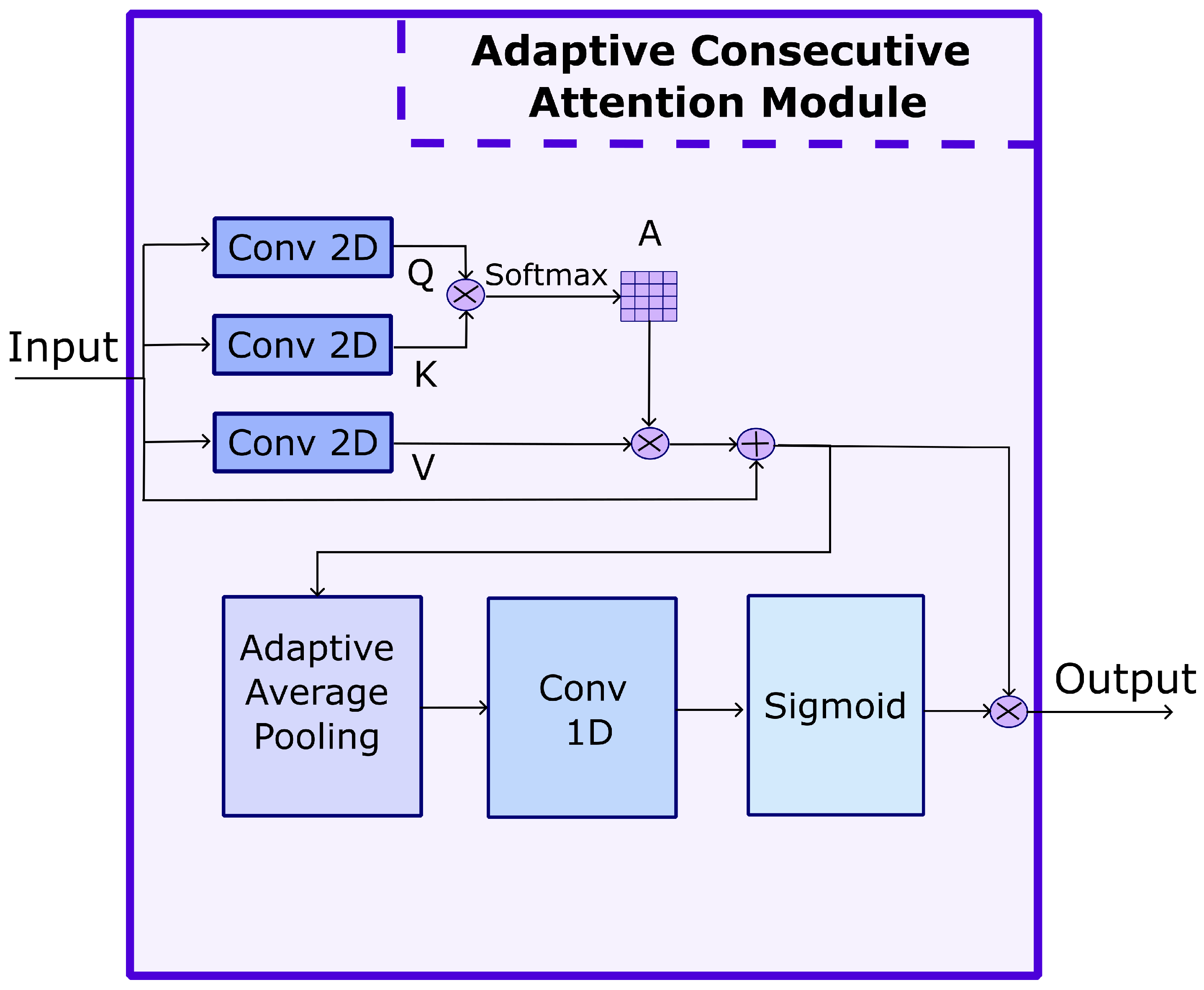Inspired by [29,35,36], a dedicated adaptive consecutive attention module (ACAM) is proposed. The CAM captures both positional and channel-related information of input features. The overall goal of this module is to systematically integrate attention mechanisms to enhance the representational capacity of the network, focused on spatial relationships and channel dependencies. The overall structure of the ACAM is depicted in Figure 3.

In the ACAM, the input $I\in {\mathbb{R}}^{C\times T\times N}$ first passes through three $Conv2D$ layers, to obtain new feature maps for query (Q), key (K), and value (V) Equation (5).

$$\begin{array}{c}\hfill Q=Conv2D\left(f_{in}\right)\\ \hfill K=Conv2D\left(f_{in}\right)\\ \hfill V=Conv2D\left(f_{in}\right)\end{array}$$

(5)

It should be emphasized that $Q,V,K$ are in ${\mathbb{R}}^{C\times T\times L}$, where L are the learned features of the joints in the skeleton data. Due to the need to determine the attention matrix in two-dimensional space, the ACAM input should be transformed to ${\mathbb{R}}^{CxN}$, where $N=T\times L$. Based on the module input, the applied attention map $A\in {\mathbb{R}}^{N\times N}$ can be defined as in Equation (6):

$$a_{n,m}={\displaystyle \frac{exp\left(Q_m·K_n\right)}{{\sum }_{m=1}^{N}exp\left(Q_m·K_n\right)}}$$

(6)

The $a_{n,m}$ is noted as the measure of the impact at position m on position n. Then, multiplication is performed between the transpose of A and V, with the result reshaped to ${\mathbb{R}}^{C\times T\times L}$. Later this result is multiplied by a scale parameter $\lambda$, and an element-wise sum is performed with features I to obtain $H\in {\mathbb{R}}^{C\times T\times L}$ as follows in Equation (7):

$$H_n=\lambda \sum _{m=1}^N\left(a_{n,m}{V}_m\right)+I_n$$

(7)

Then, an adaptive gate is added, which dynamically scales the attention mask. This allows the model to adjust the impact of the attention mechanism in Equation (8):

$$G=\sigma \left(Conv1D\left(ReLU\left(Conv1D\left(AvgPool\left(H_n\right)\right)\right)\right)\right)$$

(8)

Finally, we take the result and perform an element-wise multiplication ⊙ with the original $H_n$ to obtain the final output $f_{out}$, as in Equation (9):

$$f_{out}=H_n\odot G$$

(9)

The consecutive attention module allows the network to focus on relevant components of the motion capture data. By applying two different attention mechanisms consecutively, the module moves across spatial and channel dimensions. This is possible by using information of the relationships between features from different channels. This contextual integration enriches the network’s comprehension of tennis motion data representation and allows for a more invested representation.

5.4. Model Architecture

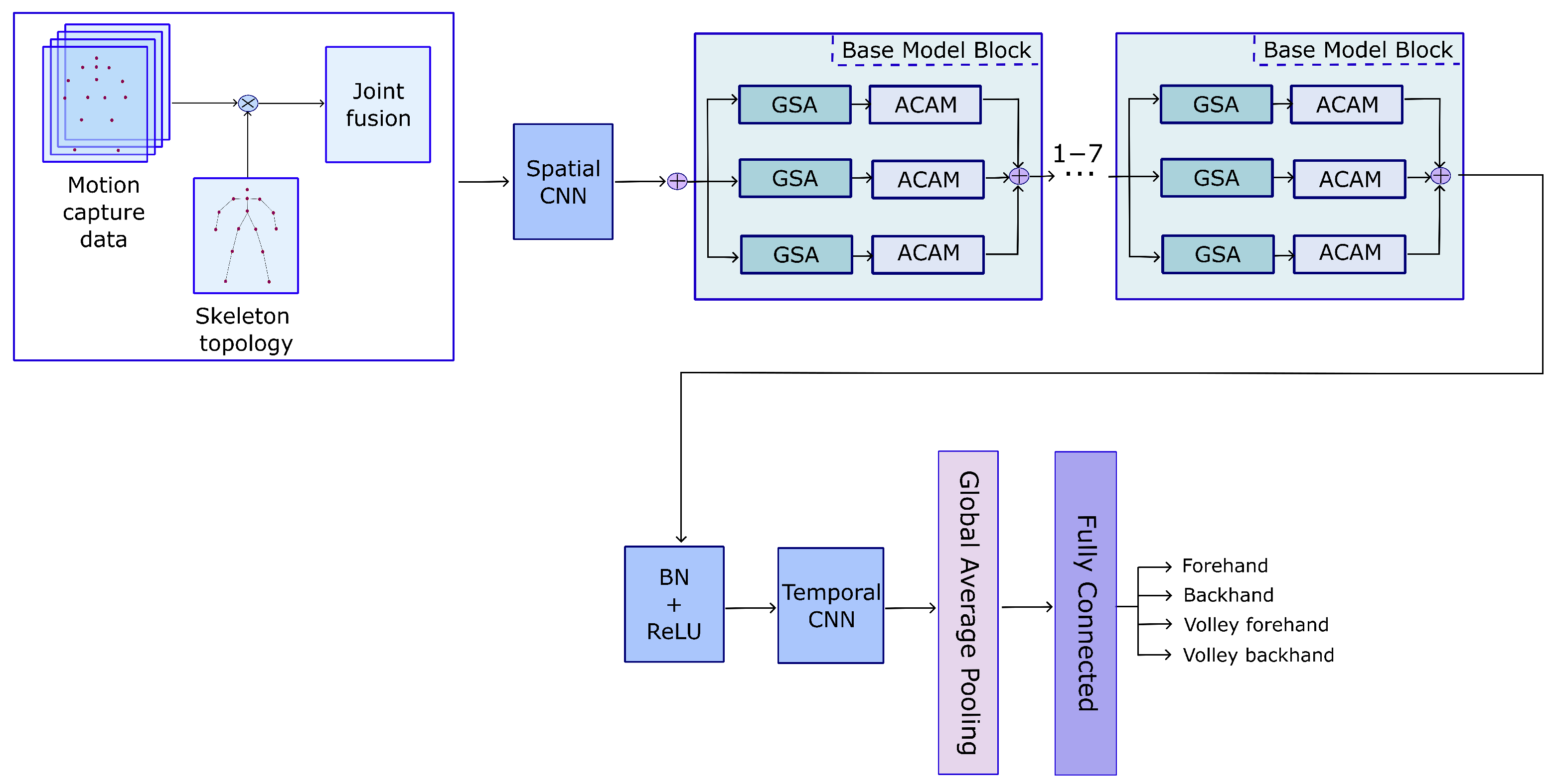
Three specialized modules are introduced for the classification of tennis strokes based on skeletons. They can be arranged either sequentially or in parallel, to form the basic building blocks of the proposed model. The graph self-attention module captures and extracts spatial as well as long-term temporal information from the skeletal joints. Moreover, information of the relationships between features from different channels is added by the adaptive consecutive attention model. Short-term temporal dependencies are multi-scale modeled by a temporal convolutional network that contributes complementary temporal cues. In addition, the Joint Motion module identifies which joints are in motion versus which remain stationary, guiding the graph self-attention to emphasize “salient” joints. Although these three modules function independently, they are closely interrelated. The complete model comprises seven stacked basic blocks, and the model architecture is outlined in

Table 1. Detailed information about the model structure.

Block No.	Layer Size	Output Shape
Input	$(3,1)$	$25\times 64\times 64$
Block 1	$(64,1)$	$25\times 64\times 64$
Block 2	$(64,1)$	$25\times 64\times 64$
Block 3	$(128,1)$	$25\times 32\times 128$
Block 4	$(128,1)$	$25\times 32\times 128$
Block 5	$(256,1)$	$25\times 16\times 256$
Block 6	$(256,1)$	$25\times 16\times 256$
Block 7	$(256,1)$	$25\times 16\times 256$
Global average pooling	-	$1\times 1\times 256$
Fully connected with Softmax	-	4-classes

and Figure 4. In Table 1, each layer describes the input channels and temporal stride, as well as the output channels. Each basic block contains three graph self-attention modules, three adaptive consecutive attention modules, and one temporal modeling module. In blocks 3 and 6, the number of channels is doubled and the temporal dimension is reduced. Each block begins with either a $(1\times 1)$ convolution or a motion fusion operation that increases the dimensionality of the input channel. Three parallel graph self-attention modules connected with adaptive consecutive attention modules are employed to extract joint information at different scales. Their outputs are summed to produce the final feature representation.

Moreover, the module integrates multi-scale temporal information, and the operation that reduces the time dimension is accomplished via depth-wise convolution. Finally, after traversing all basic layers, average pooling compresses the feature map, followed by classification of the resulting features using a fully connected layer.

5.5. Fusion Strategy

To produce the value of the input feature $f_{in}$, a feature transformation $F_L$ is defined. The objective of this transformation is to map shallow representations onto more advanced ones, formally expressed as in Equation (10):

$$F_l\left(f_{i}n\right)=M_V\left(f_{i}n\right)=V^{*}$$

(10)

where $M_V$ is defined as a matrix of value $C_{in}\times C_{out}$ size. C denotes the channels, and $V^{*}$ represents the 3D matrix of $C_{out}\times T\times N$. Due to the fact that human skeletons are highly compact data representations, a conventional self-attention mechanism can easily overfit. To mitigate this issue, we enhance the processes for extracting the query and key, adapting them more effectively to skeleton data. A linear projection is employed to reduce the channel dimensionality, thereby limiting the redundancy and computational complexity. This operation is denoted by $F_M$, mathematically described as in Equation (11):

$$\begin{array}{c}\hfill LeakyReLU\left(BN\left(F_M\left(f_{in}\right)\right)\right)=LeakyReLU\left(BN\left(M_Q\left(f_{in}\right)\right)\right)=K^{*}\\ \hfill LeakyReLU\left(BN\left(F_M\left(f_{in}\right)\right)\right)=LeakyReLU\left(BN\left(M_K\left(f_{in}\right)\right)\right)=Q^{*}\end{array}$$

(11)

Here, $BN$ denotes batch normalization, which ensures a consistent data distribution.

The learnable matrices $M_K,M_Q\in {\mathbb{R}}^{C_{in}\times C_l}$ project the input $f_{in}$ onto $Q^{*}$ and $K^{*}$. $C_l$ denotes the one-layer channel dimension (see Section 5.2 and Figure 2). Moreover, the projection of Q is divided by the number of channels, to enable to model temporal dependencies $Q=[Q_1,Q_2,\dots ,Q_l],Q_i^{*}\in {\mathbb{R}}^{T\times N}$. Furthermore, a correlation modeling function $F_H$ is introduced. Its task is to aggregate the temporal information within each channel, making it possible to capture time dependencies in the skeleton sequences. $Q_i$ and $K_i$ are obtained by applying $F_H$ to $Q_i^{*}$ and $K_i^{*}$ as in Equation (12):

$$\begin{array}{c}\hfill F_H\left(K_i^{*}\right)=\sum _{t\in T}{K}_{it}^{*}{C}_{kt}^i=K_i\\ \hfill F_H\left(Q_i^{*}\right)=\sum _{t\in T}{Q}_{it}^{*}{C}_{qt}^i=Q_i\end{array}$$

(12)

$Q_i$ and $K_i$ are the query and key vectors. Each channel i is associated with a learnable parameter set $C_i$, which fuses skeletal joint features from multiple time frames. After this temporal aggregation, the input features become $Query\in {\mathbb{R}}^{C_l\times 1\times V}$ and $Key\in {\mathbb{R}}^{C_l\times 1\times V}$. In addition, we employ an adaptive parameter map (APM) that captures static joint relationships via channels, similarly to an attention map indicating how strongly joints are connected. Next, the APM is fused with the dynamic topology derived from graph self-attention to form an updated topological structure among joints, Equation (13):

$$H=F_R(GS{A}_{map},APM)=GS{A}_{map}\times \delta +APM$$

(13)

Here, $\delta$ is a learnable parameter. Its role is to regulate the impact of the graph self-attention map ($GS{A}_{map}$). This fusion generates a channel-specific topology map for each output channel, each reflecting how the joints connect when the object is in motion. Finally, the channel topology maps from the value and fusion maps are aggregated by splitting them into $V=[V_1,V_2,\dots ,V_{out}]$ and $F=[F_1,F_2,\dots ,F_{out}]$, where $V_i\in {\mathbb{R}}^{T\times V}$ and $F_i\in {\mathbb{R}}^{V\times V}$. Each pair of channels is then aggregated as follows, Equation (14) [29]:

$$Z_i=V_i·F_i$$

(14)

Here, · denotes matrix multiplication, and $Z=[Z_1,Z_2,\dots Z_{out}]\in {\mathbb{R}}^{C_{out}\times T\times V}$ represents the final features output.

5.6. Temporal Convolutional Network

Previous works have used Temporal Convolutional Networks (TCNs) extensively in SOTA models for temporal feature extraction [37,38,39]. According to [29], this module has two main limitations. First, it has problems in detecting temporal dependencies. Second, the applied convolutions can create discontinuous temporal features with respect to the smooth motion representation in the skeleton data. Therefore, taking inspiration from [29], we decided to use a system that combines 3D spatial feature extraction with a 1D temporal convolution module for feature representation derived from skeleton-based joint data. Its structure is depicted in Figure 5.

A TCN is introduced as a novel 1D temporal convolution module which smoothly models short-term dependencies across different scales. The TCN consists of four branches $MaxPool$ and a $1\times 1$ convolution branch. The first two such branches halve the number of channels through $1\times 1$ convolutions to reduce the computational load. Depth-wise convolutions are then applied to extract multi-scale temporal features. In the third layer, the number of channels is halved again and a $MaxPool$ layer is added following the $1\times 1$ convolution in the third column. Finally, all four branches are concatenated to match the original input–output specifications. Crucially, the applied TCN does not increase the overall complexity.

5.7. Grad-CAM

To generate a Grad-CAM visualization, a specific target class is selected to interpret the model’s decision. A Grad-CAM applies the gradients of the class score (the output for the selected class) with respect to the feature maps of a chosen convolutional layer, often the last convolutional layer, during a backward pass. The derivative of the class score with respect to these feature maps indicates how the final prediction changes if the feature map values are adjusted, thus revealing each feature map’s contribution to the output. The gradients are then globally averaged (pooled) across the height and width of the feature maps, producing a weight for each feature map. These weights form the basis for creating a coarse localization map, as in Equation (15) [40]:

$${\alpha }_i={\displaystyle \frac{1}{N}}\sum _k\sum _j{\displaystyle \frac{\partial y^c}{\partial A_{kj}^i}}$$

(15)

In Equation (15), ${\alpha }_i$ indicates the weight for feature map i. N is the number of pixels in the map, $\partial y^c$ represents the score value for c class, and $\partial A_{kj}^i$ denotes the activation of the i-th feature map at location $(k,j)$. A weight is added for each feature map that represents its importance in the context of the target class. Each feature map is multiplied by its respective weight, and the weighted feature maps are summed to obtain a single two-dimensional heatmap, as in Equation (16) [40]:

$$\mathrm{Grad}-\mathrm{CAM}=\mathit{ReLU}\left(\sum _i{\alpha }_i{A}^k\right)$$

(16)

A $ReLU$ activation function is used to emphasize positive contributions, generating a heatmap that highlights key regions for the target class. This heatmap can be normalized to map its values to the range $[0,1]$, enhancing its visualization. Afterward, the heatmap is resized to align with the dimensions of the original input image. Finally, it is superimposed onto the original image, often using a color map to represent areas of greater significance.

6. Experiments and Results

In order to verify the potential of the created model, a series of experiments were performed applying the ST-GCN classifier in comparison with the FFGCAN. The well-known THETIS, Tennis-Mocap, and 3DTennisDS datasets were compared in order to verify how various types of data acquisition affected the accuracy of the human action recognition. In this study, all ONI files from THETIS, all bvh files from Tennis-Mocap, as well as all c3d data from 3DTennisDS consisting forehand, backhand, volley forehand, and volley backhand were taken into consideration. The experiment was as follows:

• Create predefined classes.
• Create simplified models of all motion capture data, divided into four strokes (corresponding to the classes).
• Create training, validation, and test sets, containing 70%, 15%, and 15% of all data, respectively.
• Train the network based on the training and validation sets.
• Test the network—five trials.
• Create a confusion matrix and compute selected measures (17)–(20) [24].

  $$Acc={\displaystyle \frac{Numberofcorrectclassifications}{Totalnumberofclassifications}}$$

  (17)

  $$Prec={\displaystyle \frac{TP}{TP+FP}}$$

  (18)

  $$Rec={\displaystyle \frac{TP}{TP+FN}}$$

  (19)

  $$F1={\displaystyle \frac{2\ast Prec\ast Rec}{Prec+Rec}}$$

  (20)

  where $TP$ refers to the true positive fraction, $FP$ refers to the false positive fraction, and $FN$ refers to the false negative fraction.

To assess the robustness and generalization capability of the proposed model, five independent experiments were conducted. Each involved a random and player-independent division of the dataset into training, validation, and test subsets. Following each run, the performance metrics were recorded. The standard deviation was computed as the square root of the variance, reflecting the statistical dispersion of individual results around the mean value. This procedure quantifies the variability in model performance attributable to different random splits of the data. No uncertainty matrix based on initial or boundary conditions was employed. The evaluation of uncertainty was restricted to a statistical analysis of repeated independent experiments. Thus, the reported standard deviations characterize the consistency of the model’s performance across various random samplings, rather than the uncertainty within a single experimental condition.

The obtained results are gathered in

Table 2. Obtained accuracy results for individual strokes based on a typical spatial-temporal graph convolutional network.

Dataset	Stroke	Mean	Max	Min	±SD
THETIS	Forehand	73.21%	80.00%	68.39%	3.26%
	Backhand	73.47%	79.37%	68.02%	3.49%
	Volley forehand	75.44%	79.85%	70.14%	3.51%
	Volley backhand	74.08%	80.00%	68.46%	3.57%
Tennis-Mocap	Forehand	76.98%	85.50%	73.05%	2.47%
	Backhand	77.10%	81.61%	73.23%	3.01%
	Volley forehand	78.13%	81.98%	73.30%	3.10%
	Volley backhand	77.79%	81.55%	73.11%	2.47%
3DTennisDS	Forehand	80.91%	85.93%	76.43%	2.78%
	Backhand	80.39%	85.81%	77.05%	3.20%
	Volley forehand	81.58%	85.94%	76.44%	2.93%
	Volley backhand	81.09%	85.22%	76.17%	2.98%

,

Table 3. Obtained precision results for individual strokes based on a typical spatial-temporal graph convolutional network.

Dataset	Stroke	Mean	Max	Min	±SD
THETIS	Forehand	79.30%	84.21%	74.19%	2.75%
	Backhand	77.64%	82.47%	72.63%	2.70%
	Volley forehand	73.34%	79.21%	68.32%	3.28%
	Volley backhand	72.60%	78.34%	67.00%	3.40%
Tennis-Mocap	Forehand	81.81%	85.91%	77.86%	2.72%
	Backhand	77.40%	81.88%	73.51%	2.94%
	Volley forehand	75.84%	80.67%	71.05%	3.20%
	Volley backhand	78.49%	82.88%	73.97%	2.94%
3DTennisDS	Forehand	85.60%	88.54%	81.05%	2.33%
	Backhand	84.46%	87.63%	80.21%	2.53%
	Volley forehand	80.96%	84.16%	73.24%	2.57%
	Volley backhand	81.17%	85.86%	75.49%	3.60%

,

Table 4. Obtained recall results for individual strokes based on a typical spatial-temporal graph convolutional network.

Dataset	Stroke	Mean	Max	Min	±SD
THETIS	Forehand	70.55%	76.92%	65.09%	3.51%
	Backhand	76.10%	80.81%	71.88%	2.75%
	Volley forehand	79.81%	84.21%	74.19%	2.87%
	Volley backhand	76.62%	82.47%	71.13%	3.10%
Tennis-Mocap	Forehand	74.70%	79.74%	70.78%	3.23%
	Backhand	83.04%	86.52%	79.56%	2.23%
	Volley forehand	79.21%	84.02%	75.00%	3.12%
	Volley backhand	76.85%	81.21%	72.08%	3.20%
3DTennisDS	Forehand	79.85%	85.00%	72.64%	4.01%
	Backhand	82.38%	85.00%	78.58%	2.20%
	Volley forehand	85.83%	89.47%	81.91%	2.26%
	Volley backhand	84.21%	87.50%	79.38%	2.58%

,

Table 5. Obtained F1-score results for individual strokes based on a typical spatial-temporal graph convolutional network.

Dataset	Stroke	Mean	Max	Min	±SD
THETIS	Forehand	74.66%	80.40%	69.35%	3.17%
	Backhand	76.86%	81.63%	72.25%	2.68%
	Volley forehand	76.44%	81.63%	71.13%	3.02%
	Volley backhand	74.55%	80.40%	69.00%	3.24%
Tennis-Mocap	Forehand	78.09%	82.71%	74.15%	3.00%
	Backhand	80.12%	84.14%	76.76%	3.56%
	Volley forehand	77.48%	82.31%	72.79%	3.16%
	Volley backhand	77.66%	82.03%	73.22%	4.06%
3DTennisDS	Forehand	82.61%	86.73%	76.62%	3.22%
	Backhand	83.41%	86.29%	79.38%	2.35%
	Volley forehand	83.32%	86.73%	78.97%	2.41%
	Volley backhand	82.65%	86.29%	77.39%	3.08%

,

Table 6. Obtained accuracy results for individual strokes based on the proposed model.

Dataset	Stroke	Mean	Max	Min	±SD
THETIS	Forehand	91.82%	94.29%	85.44%	4.08%
	Backhand	90.66%	96.66%	84.19%	3.87%
	Volley forehand	90.04%	97.87%	88.29%	4.04%
	Volley backhand	96.84%	98.52%	87.17%	4.87%
Tennis-Mocap	Forehand	92.64%	97.63%	90.15%	2.92%
	Backhand	93.17%	95.39%	88.51%	3.50%
	Volley forehand	91.27%	93.75%	89.46%	2.13%
	Volley backhand	92.22%	95.28%	85.51%	2.10%
3DTennisDS	Forehand	95.64%	97.31%	86.69%	3.38%
	Backhand	95.77%	98.14%	91.70%	3.17%
	Volley forehand	94.93%	96.19%	93.50%	2.27%
	Volley backhand	94.26%	98.79%	87.51%	2.94%

,

Table 7. Obtained precision results for individual strokes based on the proposed model.

Dataset	Stroke	Mean	Max	Min	±SD
THETIS	Forehand	94.43%	96.51%	91.93%	3.43%
	Backhand	93.26%	97.48%	92.35%	2.17%
	Volley forehand	91.37%	94.87%	87.58%	3.93%
	Volley backhand	94.27%	97.45%	85.25%	4.03%
Tennis-Mocap	Forehand	92.40%	96.30%	90.43%	3.38%
	Backhand	91.92%	97.93%	89.40%	3.77%
	Volley forehand	93.46%	96.97%	86.31%	3.94%
	Volley backhand	92.08%	95.91%	90.54%	3.56%
3DTennisDS	Forehand	94.98%	98.61%	93.09%	2.66%
	Backhand	92.62%	94.97%	89.41%	3.84%
	Volley forehand	94.39%	97.07%	90.18%	2.98%
	Volley backhand	92.77%	95.07%	90.86%	4.03%

,

Table 8. Obtained recall results for individual strokes based on the proposed model.

Dataset	Stroke	Mean	Max	Min	±SD
THETIS	Forehand	89.68%	96.18%	77.57%	4.28%
	Backhand	91.73%	94.93%	86.56%	3.33%
	Volley forehand	91.64%	97.16%	80.81%	3.36%
	Volley backhand	93.46%	96.52%	85.43%	3.71%
Tennis-Mocap	Forehand	92.15%	95.74%	86.42%	3.80%
	Backhand	92.37%	96.28%	88.98%	2.59%
	Volley forehand	91.62%	95.39%	83.65%	3.63%
	Volley backhand	92.02%	95.15%	89.91%	4.15%
3DTennisDS	Forehand	93.36%	96.01%	89.19%	5.13%
	Backhand	90.82%	93.82%	86.59%	3.63%
	Volley forehand	95.62%	97.44%	83.73%	2.68%
	Volley backhand	93.53%	97.67%	88.13%	3.13%

and

Table 9. Obtained F1-score results for individual strokes based on the proposed model.

Dataset	Stroke	Mean	Max	Min	±SD
THETIS	Forehand	90.22%	95.39%	79.31%	3.64%
	Backhand	90.90%	96.59%	84.27%	3.31%
	Volley forehand	91.47%	96.28%	89.71%	3.69%
	Volley backhand	91.71%	92.12%	79.83%	4.67%
Tennis-Mocap	Forehand	94.27%	97.72%	90.91%	3.40%
	Backhand	93.51%	96.82%	86.97%	4.28%
	Volley forehand	92.08%	97.67%	89.72%	3.77%
	Volley backhand	91.46%	95.48%	83.37%	4.77%
3DTennisDS	Forehand	91.09%	96.76%	89.31%	3.68%
	Backhand	92.63%	96.30%	89.91%	3.80%
	Volley forehand	92.39%	96.26%	90.31%	2.68%
	Volley backhand	93.77%	95.92%	88.33%	3.87%

. Moreover, confusion matrices are depicted in Figure 6, with the course of the learning process in Figure 7.

The proposed model was developed based on PyTorch 2.2. The training and testing were conducted on a work station with AMD Ryzen Threadripper PRO 7965WX, as well as a single NVIDIA RTX 4090 GPU. The momentum was SGD, the Adam optimizer was set to $0.001$, $\beta 1=0.9$, $ϵ={10}^{-8}$. The epochs were set to 60, and model warm up was the first 5 epochs. An early stop procedure was used after 5 epochs without any improvement. The learning rate was 0.1, and at epoch 40 the learning rate decayed by a factor of 0.1. The batch size was 64 data points.

Computational Efficiency

The proposed FFGCAN had only 1.33 M parameters and required 2.746 GFLOPs per $200\times 17$ sequence. On the GPU (RTX 4090) it achieved 0.96 ms latency, which corresponds to ≈$1041FPS$ and allowed for smooth real-time inference. Compared to the baseline ST-GCN, we had ≈22.65% fewer FLOPs and a ≈45.5% shorter processing time, with incomparably higher accuracy. The obtained computational efficiency results are presented in

Table 10. Comparison of inference complexity and speed for the baseline models (ST-GCN) and the proposed FFGCAN. The time measurement was performed on RTX 4090 and a single-core Ryzen 7950X with the sequence $T=200$, $V=17$.

Model	Param. [M]	GFLOPs	RTX 4090 Latency [ms]	CPU Latency [ms]
ST-GCN	3.10	3.55	1.83	9.55
FFGCAN (our)	1.33	2.746	0.96	5.4

and

Table 11. FLOPS for a single sequence $T=200,V=17$. Values are in millions of floating-point operations (GFLOPS).

No.	Layer	Configuration	FLOPS [G]	Part
Stem
1	Conv2d $1\times 1$	$3\to 64$	0.75	0.03%
Blocks 1–3 ($64\to 64$)
2	3 × GSA	64	49.06	1.8%
3	3 × ACAM	64	6.16	0.2%
4	3 × TCN	64	0.11	≪0.1%
Blocks 4–5 ($64\to 128$)
5	2 × GSA	128	130.94	4.8%
6	2 × ACAM	128	16.37	0.6%
7	2 × TCN	128	0.15	≪0.1%
Blocks 6–7 ($128\to 256$)
8	2 × GSA	256	524.38	19.1%
9	2 × ACAM	256	65.31	2.4%
10	2 × TCN	256	0.31	≪0.1%
GAP + FC
11	Global AvgPool	—	—	—
12	FC $256\to 4$	—	0.006	≪0.1%
Sum			2746 G	100%

.

7. Discussion

In this study, a new model, called the Feature Fusion Graph Consecutive-Attention Network, was proposed for tennis movement recognition. The basic strokes were detected, such as forehand, backhand, volley forehand, and volley backhand. The model incorporates seven basic blocks that are combined with two types of module: an Adaptive Consecutive Attention module, and Graph Self-Attention module. They are employed to extract joint information at different scales from motion capture data. The consecutive attention module allows the network to focus on relevant components. This enriches the network’s comprehension of tennis motion data representation and allows for a more invested representation. The second module captures and extracts spatial and long-term temporal information from skeletal joints. The temporal convolutional network is applied to identify short-term temporal dependencies. The FFGCAN utilizes a fusion of motion capture data that generates a channel-specific topology map for each output channel, reflecting how the joints are connected when the tennis player is moving.

The proposed model was verified using three well-known motion capture datasets containing basic tennis moves. They contain the positioning of the player’s silhouette while performing strokes with different representations and with various quantities of three-dimensional data. That is why the Tennis-Mocap and 3DTennisDS data were simplified to the THETIS model. It should be noted that the 3DTennisDS dataset contains additional data of the tennis racket, which were also incorporated in this study.

The suggested Feature Fusion Graph Consecutive-Attention Network was compared with a Spatial-Temporal Graph Convolutional Network, which is often applied for identifying human actions. This network is very often used to designate motion and appearance patterns, both from video and three-dimensional data. The obtained accuracy results for the ST-GCN proved that this type of model is suitable for accurate tennis movements recognition (Table 2). It is clear that the network performance depended on the type of input data. The lowest accuracy results were obtained for motion capture data registered from the markerless system, from the THETIS dataset. The tennis stroke recognition performance ranged from 73.21% to 75.44%. Tennis stroke recognition based on data from the Tennis-Mocap dataset achieved a slightly higher efficiency, from 76.98% to 78.13%. The highest accuracy results for tennis stroke recognition for the ST-GCN were obtained for data from the 3DTennisDS dataset, slightly above 80%. The precision results obtained for the ST-GCN proved that this solution is accurate and avoids false positives (Table 3). It also usually correctly identified positive instances from all actual positive samples (Table 4). The predictive skill of the ST-GCN model was high, exceeding 74%, given by the F1-score results (Table 5). The proposed new FFCGAN network was characterized by a very high efficiency in recognizing tennis strokes. The obtained accuracy results exceeded 90% for each analyzed dataset, regardless of the type of input data (Table 6). The proposed classifier recognized tennis strokes proficiently. It should be noted that both the ST-GCN network and the new model had very low standard deviation values, which confirms their stability. The FFCGAN model obtained very high precision results, above 91%, which proves that the model dealt excellently with false positive samples (Table 7). The recall results for the proposed model also reached very high values, exceeding 89.68% (Table 8). This indicates that the network correctly recognized the positive samples. The obaitned harmonic mean values of precision and recall for the FFCGAN were higher than 91%, which shows that the network has excellent predictive skills (Table 9).

The confusion matrices obtained for the ST-GCN and the FFCGAN provide a more comprehensive insight into the performance of the compared models. It can be seen that the forehand and backhand strokes were misclassified as their volley equivalents and vice versa (Figure 6). It should be emphasized that the proposed model significantly reduced the confusion of these tennis shots, by up to 70%.

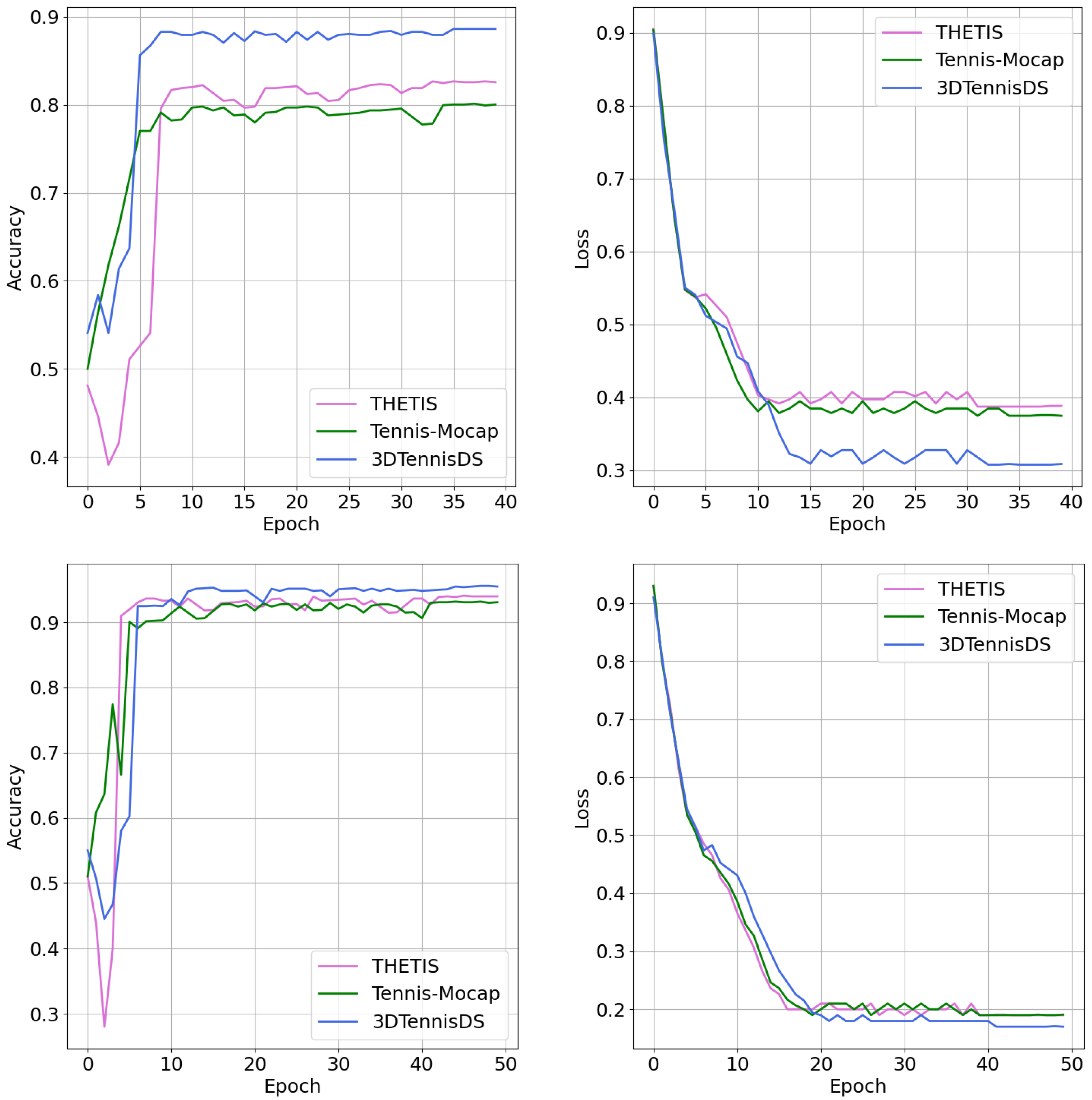
Analyzing the learning curves and loss functions of the ST-GCN and FFCGAN models, it can be concluded that both solutions were stable (Figure 7). The ST-GCN network achieved stability after 40 epochs. While the network proposed by the authors needed slightly longer, at 50 epochs. This is a comparable number. It should be noted that in the case of the FFCGAN, the obtained effectiveness was comparable for all analyzed datasets, while for the ST-GCN network, significant differences can be observed. The FFCGAN model achieved more accurate predictions.

Taking into account all the results, it should be stated that the developed tool, FFCGAN, was extremely effective in recognizing tennis strokes based on three-dimensional data acquired from different types of motion capture systems. This universal tool will allow increasing the effectiveness of recognizing basic tennis strokes.

7.1. Comparison with the State of the Art

Spatial-temporal dependencies in motion capture data are crucial for action recognition performance. Sequence-vision-based data may suffer from the inconsistency in trajectories, which further results in misleading classification [41,42]. Many deep learning models disregard the relationships between frames in dynamic movements, and thus long-term temporal dependencies are not sufficiently provided [43,44]. In many studies, the motion capture data were split into an equal length set of frames, which may cause a loss of key information [45]. Usually, these kinds of data are registered utilizing systems calibrated for specific types of movements. In order to eliminate the above weaknesses, the Feature Fusion Graph Consecutive-Attention Network (FFGCAN) was proposed.

It was compared with other models that were applied for three tennis motion capture datasets, THETIS, Tennis-Mocap, and 3DTennisDS (

Table 12. Comparison with state-of-the-art studies involving three tennis motion capture datasets.

Study	Dataset	Model	Accuracy
[13]	THETIS	LSTM	81.23–89.42%
		SVM	51.20%
[8]	THETIS	Deep Historical LSTM	62%
[12]	THETIS	LSTM	70.17–97.67%
[33]	THETIS	SVM	53.08–60.23%
[24]	THETIS	ST-GCN	73.21–75.47%
		ST-GCN with fuzzy input	80.10–81.43%
[24]	Tennis-Mocap	ST-GCN	76.98–78.13%
		ST-GCN with fuzzy input	81.20–84.62%
Our	THETIS	FFGCAN	90.04–96.52%
[17]	THETIS and Tennis-Mocap	ASE-CNN	up to up to 98%
Our	Tennis-Mocap	FFGCAN	91.27–93.17%
[23]	3DTennisDS	ST-GCN	64.10–74.30%
		ST-GCN with fuzzy input	86.30–87.30%
[24]	3DTennisDS	ST-GCN	80.39–81.58%
		ST-GCN with fuzzy input	85.42–87.97%
[26]	3DTennisDS	A3T-GCN	74.22–81.95%
		A3T-GCN with fuzzy input	86.90–93.82%
[27]	3DTennisDS	DA-GCN	89.79–91.38%
[25]	3DTennisDS	A3T-GCN	88.41–89.84%
Our	3DTennisDS	FFGCAN	94.26–95.77%

). The SOTA results confirm that the proposed model was exceptionally effective in recognizing tennis strokes, regardless of the type of input data, gathered by markerless systems or passive optical ones. The FFGCAN was characterized by much higher performance, outperforming DL models such as LSTM, but also ST-GCNs. The obtained accuracy results are higher than in the case of input data fuzzification for classifiers based on graph neural networks. It is worth stressing that the proposed solution outperformed graph models with attention modules applied.

7.2. Explainable AI

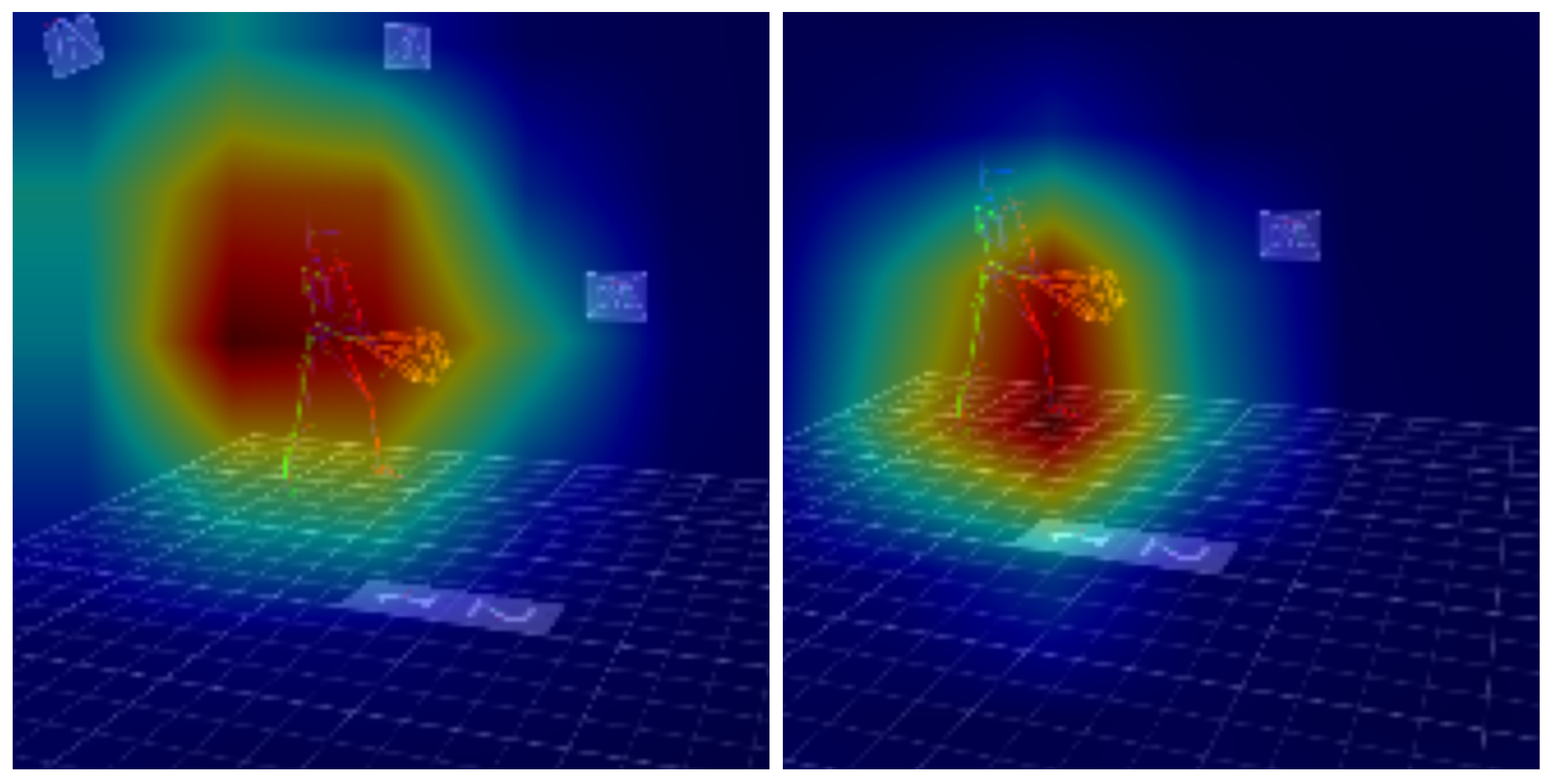
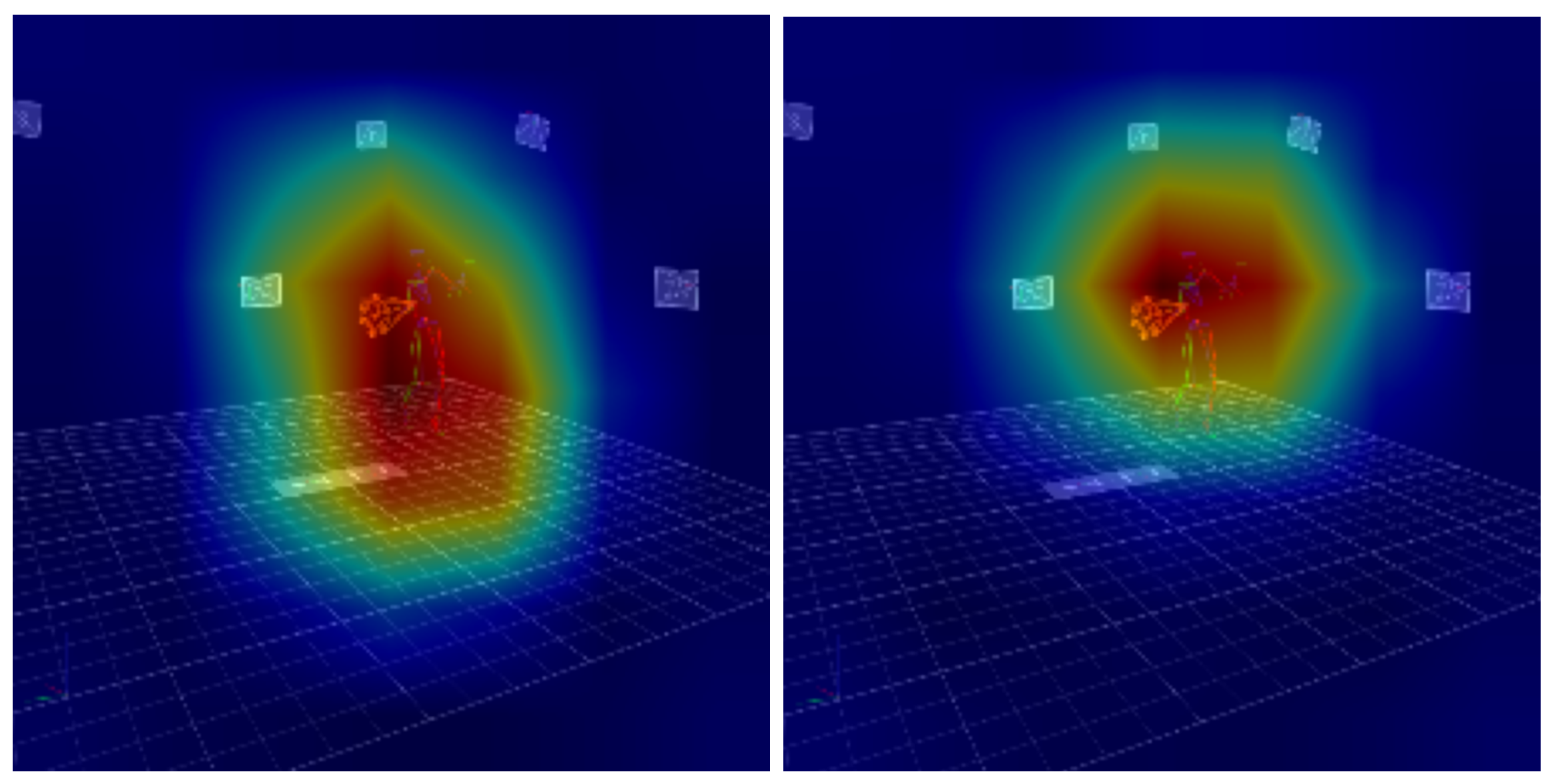
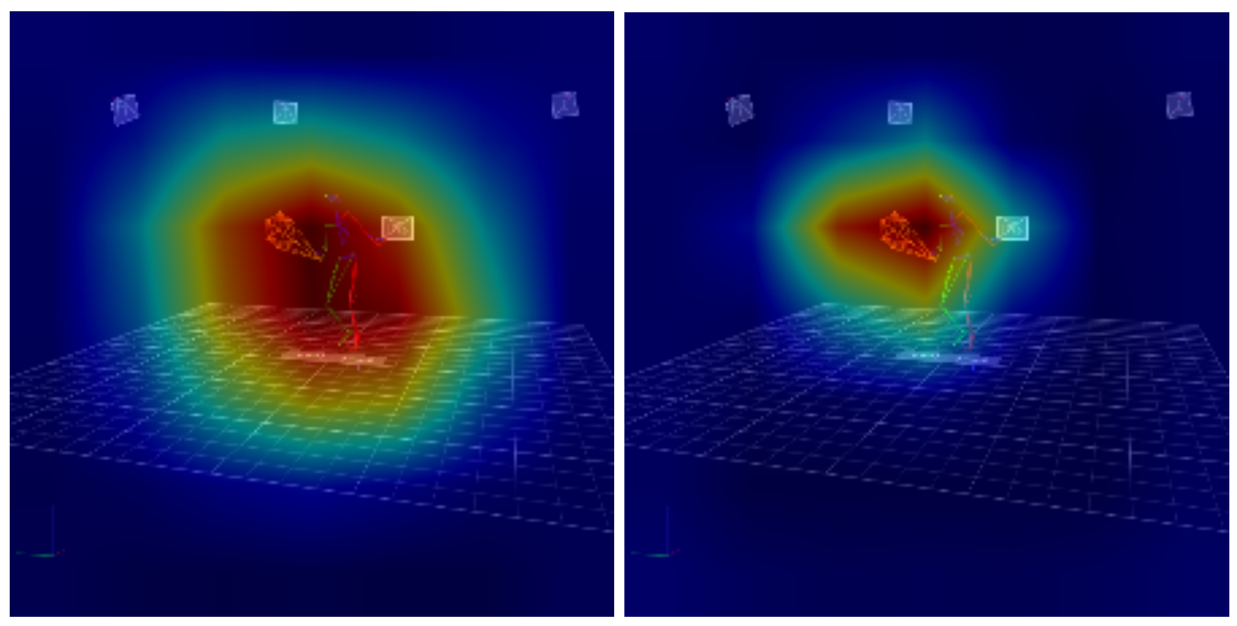
In order to show the elements of the model’s effectiveness and to visualize the elements taken into account in the classification of tennis strokes, the grad-CAM technique was used. Due to the fact that it operates only on a point cloud, the corresponding images from the VICON system are displayed as a background for the generated heat maps.

It should be emphasized that the background images in Figure 8, Figure 9, Figure 10 and Figure 11, depicting a player executing a specific type of stroke, serve solely illustrative purposes and do not convey the dynamic nature of the recorded motion. The model under discussion was constructed using motion capture data, recording the spatial coordinates of markers in three-dimensional space over time. As a result, the Grad-CAM visualizations may appear to suggest substantial errors. However, these discrepancies arose from the natural variability in the player’s movement, rather than from inaccuracies in the model itself. It is important to note that Grad-CAM identifies regions of the input data that are most critical for the classification of the entire stroke, not of a single frame. In contrast, the background image corresponds to a single frame extracted from the analyzed stroke. The warmer colors (red, orange, yellow) mark regions that most increased the model’s confidence in the chosen class, while cooler colors (blue, green) had margin or no positive influence.

The analysis of the Grad-CAM visualization for the ST-GCN and FFCGAN models showed how both models tracked the player’s movement during tennis strokes in a different way. The visualization for the FFCGAN model shows a much more concentrated, spatial activation, located mainly in the lower body and at the point of contact between the racket and the ball. It should be noted that the image visible as a background does not reflect the movement sequence, but presents a single frame in a static form. This suggests that the FFCGAN model primarily pays attention to the movements of the legs and racket that generate the stroke. On the other hand, the visualization for the ST-GCN model shows an activation that is quite broad, covering almost the entire player’s silhouette, with the surroundings. It can be stated that the ST-GCN model integrates a wide movement context, taking into account the dynamics of the whole body and wider spatial relationships. It should be noted that footwork is crucial in performing tennis strokes. It can therefore be assumed that the adaptive spatio-temporal attention modules used in the FFCGAN model allow capturing more complex relationships between the individual biomechanical elements of tennis movement.

8. Conclusions and Future Works

Although the proposed model achieved state-of-the-art performance on three publicly available motion-capture datasets, several factors may currently limit its robustness.

• Sensitivity to missing or occluded data
  All graph–based skeleton models implicitly assume complete and correctly connected joint graphs. Frames in which markers are either lost or merged in the 2-D projection (overlapping nodal lines) degrade the quality of the adjacency matrix and cannot be recovered solely by the attention mechanism. In such cases, the model inherits the errors of the upstream pose-estimation pipeline, rather than compensating for them.
• Dataset-specific topology inconsistencies
  The FFGCAN uses an additional graph node representing the racket (available in 3DTennisDS), whereas THETIS and Tennis-Mocap lack this information. Although the fusion strategy learns channel-specific topologies, cross-dataset transfer still requires retraining or domain adaptation, because the underlying joint sets differ.
• Limited kinematic diversity
  The training corpora mainly include amateur and sub-elite players performing a short list of strokes under controlled conditions. Movement variations unseen in the training process may therefore lie outside the training distribution and elicit unpredictable model behaviors.
• Computational constraints on edge hardware
  Despite the relatively small trainable features (1.33 M parameters, 2.7 GFLOPs per $200\times 17$ sequence), real-time deployment on low-power devices still demands further optimization (pruning, quantization, or knowledge-distillation). The latency measurements presented in Section 6 correspond to a high-end RTX 4090 GPU and do not directly translate to mobile or embedded platforms.
• Explaining decisions beyond coarse Grad-CAM maps
  Current interpretability relies on sequence-level Grad-CAM heatmaps, which highlight joint clusters but offer limited temporal resolution. Single-frame visualizations may appear misaligned with the heatmap because the latter integrates evidence across the entire stroke. Finer-grained temporal roll-out or attention-flow analyses may reveal how the network reasons over consecutive motion phases.

In conclusion, the proposed FFGCAN model showed significant promise for tennis action recognition, outperforming existing models. Future work should focus on enhancing data diversity, computational efficiency, and interpretability, to fully unlock its potential in real-world applications.

Despite demonstrating promising results, this study acknowledges several inherent limitations. The datasets used, THETIS, Tennis-Mocap, and 3DTennisDS, have very limited variability in the player skill levels, conditions of the environment, and scenarios of the game. Such restricted diversity might limit the generalization capability of the model regarding tennis scenarios at large. In addition, the simplification procedures used to align the Tennis-Mocap and 3DTennisDS datasets with the THETIS dataset framework inevitably reduced some detailed features. The absence of analysis related to inference times, model sizes, or computational resource requirements could affect its practical deployment in real-time or resource constrained applications.

To address these limitations, future studies could explore enhancing the dataset diversity by including a broader selection of player data, as well as testing the model on other motion capture datasets. Investigating methods to optimize computational efficiency through pruning, quantization, or knowledge distillation could also substantially enhance real-world applicability. Furthermore, enhancing interpretability beyond Grad-CAM by employing attention visualization methods would deepen our understanding of the underlying decision mechanisms.

The results proved that the proposed model is highly effective, providing new insights into HAR in tennis movement classification.