A CNN-Based Downscaling Model for Macau Temperature Prediction Using ERA5 Reanalysis Data

Abstract

Temperature is a core element of the regional climate system and plays a key role in energy exchange and weather evolution. The current reanalysis of temperature data faces difficulties in providing more accurate geographical temperature data due to insufficient spatial resolution (0.25° × 0.25°). In this study, a lightweight downscaling method incorporating a convolutional neural network is proposed to construct a high-resolution temperature prediction model for the Macau region based on ERA5 reanalysis data. Aiming at the existing data due to insufficient resolution, a two-stage convolutional feature extraction module is introduced to optimize the model parameters by combining them with the observation data of Macau meteorological stations. The experimental results show that the accuracy of this method is 21.4% higher than that of the traditional interpolation method in the instantaneous prediction, and the prediction effect in the next 3 h is also very good. The model is expected to be extended to other regions in the future, providing an effective solution for obtaining long-term high-resolution temperature data in other regions, which can support the refinement of meteorological services and climate research.

1. Introduction

As an important cornerstone of social development, the influence of modern weather forecasting has permeated many fields, including agricultural production, transportation, disaster prevention and mitigation, and public safety [1]. Nearly 150 years ago, the public weather forecasting service started the prelude of modern meteorology, and since then the discipline has taken forecasting technology as its core development direction [2]. Accompanied by the accumulation of long-term practical experience and the rapid progress of science and technology, human beings are facing the emerging new issues and increasing technical challenges in the field of meteorological forecasting in the process of continuously improving the theoretical system of atmospheric science [3].

Existing gridded temperature datasets are limited by the problem of coarse spatial resolution, which makes it difficult to meet the application needs of more fine-grained geographical temperature data. Although high-resolution atmospheric models can theoretically provide more accurate simulation data, their high computational cost makes it difficult to run them continuously for a long period of time in order to construct reliable historical datasets [4]. In contrast, reanalysis data, with the advantage of assimilation technology, can provide long-term continuous and large-scale spatial and temporal coordinated temperature field data, although the spatial resolution is relatively low, and this property makes it more useful in climate-scale studies.

Reanalysis data have a wide range of applications in atmospheric science, with ERA5 being one of the most commonly used types of reanalysis data, which covers the globe with a spatial resolution of 0.25°, spanning the period from 1940 to the present, and contains variables commonly used in the atmosphere, including temperature and pressure.

In this study, a deep learning temperature prediction model incorporating geospatial features is constructed to address the problem of insufficient spatial resolution (0.25° × 0.25°) of ERA5 reanalysis data in regional-scale applications, especially considering the current situation that special geographic units such as Macau are not in the grid nodes, resulting in the limited accuracy of traditional interpolation. There are significant bottlenecks in the current ERA5 reanalysis data. The spatial resolution of the current open datasets can hardly support the demand of urban microclimate research, especially in complex terrain areas such as Guangdong, Hong Kong, and Macau Greater Bay Area. To obtain high-spatial-resolution data, existing studies mostly use traditional spatial interpolation methods such as bilinear interpolation and cubic spline interpolation to obtain off-grid point data, but they ignore the effect of nonlinearity. For this reason, this study innovatively compares convolutional neural network (CNN) with classical interpolation methods systematically to break through the application limitations of traditional methods.

After breaking through the traditional image recognition field, the unique value of convolutional neural network (CNN) in time series prediction has gradually emerged [5]. Through the sliding scanning of the convolutional kernel in the time series dimension, CNN can adaptively extract local correlation features in the data: a small-scale convolutional kernel (e.g., 3 steps) can capture intra-day periodic fluctuations in the temperature series, whereas a large-scale convolutional kernel (e.g., 30 steps) can identify quarterly trend changes [6], which significantly improves the modeling accuracy of scenarios such as weather forecasting. Its parameter-sharing feature dramatically reduces model complexity, and the parallel convolutional operation accelerated by GPU improves the training efficiency of millions of weather station point data by 2–3 orders of magnitude, effectively alleviating the high-dimensional catastrophe problem of the traditional fully connected network [7]. In the face of heterogeneous time series data from multiple sources, CNN can synchronously analyze the cross-modal interactions of temperature, barometric pressure, humidity, and other meteorological elements by constructing a multi-dimensional tensor input layer, and it breaks through the dependence of the classical time series model on the assumption of equidistant intervals by making use of the cavity convolution technique compatible with non-uniform sampling data [8].

This study focuses on improving the spatial applicability of ERA5 reanalysis data in the Macau region. Due to the special geographic location of Macau (22.16° N, 113.57° E), which does not overlap with the ERA5 grid points, there is a systematic bias in the direct calculation of traditional interpolation methods. For this reason, we systematically compare three benchmarking methods: directly using the true value of the Macau region (Observed) with the nearest-neighbor interpolation (Nearest), bilinear interpolation (Linear), and cubic spline interpolation (Cubic) [9], and constructing a convolutional neural network (CNN) model for the spatial refinement correction. The main contributions of this research are as follows:

• In this study, based on the 2012–2020 ERA5 hourly 2 m temperature data (VAR_2T), a 41 × 41 grid dataset around Macao (17–27° N, 109–119° E) was constructed, and a CNN model was used for spatial and temporal feature extraction and prediction. The CNN model was used for spatial and temporal feature extraction and prediction, and the output values were compared with the measured temperatures at the Tai Tam Shan site of the Macau Meteorological Bureau (22.16° N, 113.57° E).
• In the methodological framework, this study compares the CNN model with three traditional interpolation methods: the ERA5 Nearest directly uses nearest-neighbor grid point temperatures; the ERA5 Linear implements bilinear interpolation based on 4-neighbor grid points; and the ERA5 Cubic performs cubic spline interpolation through 16-neighbor grid points. A baseline reference is provided for subsequent model performance analysis.

The rest of the paper is structured as follows: Section 2 briefly describes the data sources and processing methods, including the ERA5 reanalysis dataset, and the Macau ground station data; Section 3 introduces the traditional interpolation methods as well as our deep learning model; Section 4 demonstrates the experimental results and argues the advantages of deep learning over traditional methods and the potential for regional expansion; and finally, Section 5 concludes the results and looks forward to the actual business applications and multi-region extension.

2. Data

The European Centre for Medium-Range Weather Forecasts (ECMWF), as an authoritative organization in the field of global meteorological reanalysis, has gone through many generations of technological evolution in its reanalysis data product system: from laying the foundation of the first Global Atmospheric Research Program (FGGE) in 1979, to the release of the first 15-year reanalysis dataset ERA-15 (1978–1994) in the 1990s, and then the launching of the cross-century dataset ERA-40 (1957–2002) and its improved version ERA-Interim (1979–2019) [10], culminating in the current most representative fifth-generation reanalysis product, ERA5, which covers the period from January 1940 to the present, with a spatial resolution of 0.25° (about 31 km) and a temporal resolution of 1 h, including many meteorological variables, such as temperature, humidity, wind speed, etc. [11].

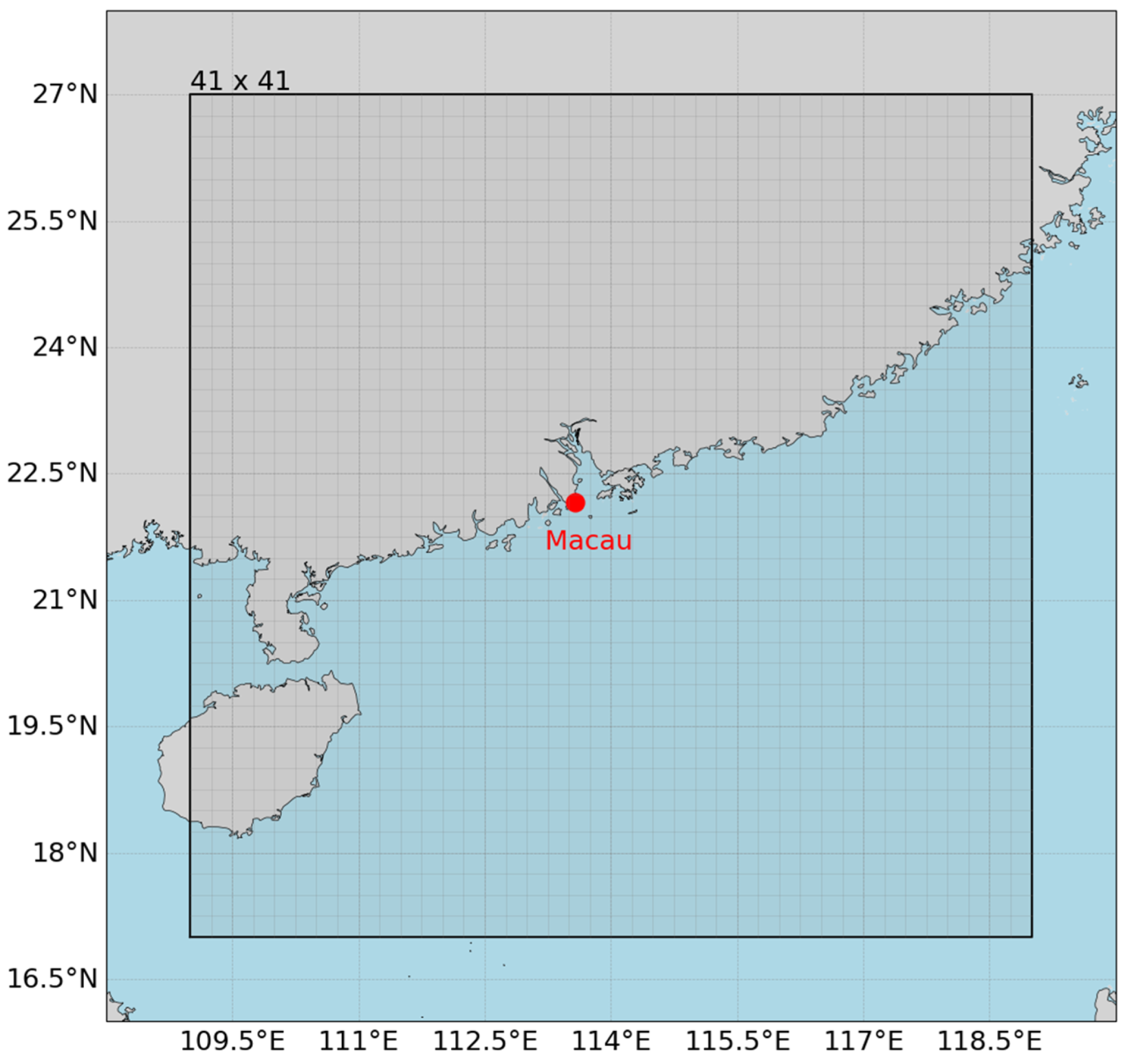
In this study, the air temperature at 2 m above the surface (variable identified as VAR_2T, hereinafter referred to as temperature) from the ERA5 for the period 2012–2022 is used. As shown in Figure 1, the data were focused on a specific range around Macau, i.e., the area covered by latitude 17–27° N and longitude 109–119° E, with a total of 41 × 41 grid points, as indicated by the intersection of the grid lines.

For Macau, a typical tropical monsoon climate zone, the ERA5 data can accurately characterize the spatial heterogeneity of its climatic features—and its high temporal resolution makes it possible to capture climatic fluctuations in short time scales, while its high spatial resolution helps to reveal the climatic differences between different regions [12], which provide a reliable data base for assessing the regional climatic evolution and its impacts on the urban operation. As an important node in the Guangdong–Hong Kong–Macau Greater Bay Area, the refined distribution data of meteorological elements in the Macau region have an important decision support value for extreme weather warning, urban planning, and ecosystem management.

The real temperature values are based on the 2012–2022 measured temperature series from the Tai Tam Shan Meteorological Station (22.16° N, 113.57° E, altitude 112 m) in Macau. The data from this station fully characterize the typical features of the subtropical monsoon climate of Macau: in summer (June–August), controlled by the subtropical high pressure, the monthly mean temperature is 28.6–31.9 °C; in winter (December–February), influenced by the East Asian winter winds, the monthly mean temperature is 16.2–19.5 °C, which constitutes the seasonal baseline validation scenario of the temperature prediction model.

In this study, two datasets are used for analysis. The ERA5 reanalysis dataset provides gridded air temperature at 2 m above the surface and is used as the model input. Observational data from the Macau meteorological station serves as the label for supervised learning.

The temperature variable in the ERA5 reanalysis data is stored in Kelvin (K), an international standard unit system. In order to adapt the observation data (unit: °C) from the Macau meteorological station, it is necessary to perform the temperature scale conversion: based on the standard formula T (°C) = T (K) − 273.15 defined by the International Committee for Weights and Measures (CIPM) [13], the vectorization operation is implemented on the dataset, and the batch conversion from Kelvin to Celsius is realized.

To solve the problem of time matching between the ERA5 reanalysis data of the European Meteorological Centre (ECMWF) and the meteorological observations of Macau, a standardized alignment method is used. Time zone and format differences are eliminated by standardizing the date format (complementary eight-digit specification) and the hourly rounding mechanism (24 o’clock is automatically converted to the next day’s 0 o’clock).

For model training and testing, the processed data are divided into a training set, validation set, and test set. Among them, the temperature data from 01:00 on 1 January 2012 to 24:00 on 31 December 2020 local time are the training set and validation set with random assignment in a ratio of 8:2, and the temperature data from 01:00 on 1 January 2021 to 24:00 on 31 December 2022 local time are the test set. After removing 14 invalid Macau real temperature values, the training set contains 63,119 samples, the validation set contains 15,780 samples, and the test set contains 17,519 samples.

3. CNN Model Construction and Training

3.1. Interpolation Methods

In grid data processing, the choice of interpolation algorithms needs to be closely coupled with the constraints of grid type (structured or unstructured), data continuity requirements, and computational efficiency. For structured grids (e.g., uniformly distributed 2D or 3D grids), traditional image interpolation methods can be directly migrated to applications. Traditional interpolation methods, such as nearest-neighbor interpolation, bilinear interpolation, and cubic spline interpolation, will be compared with deep-learning-based approaches [14,15].

Nearest-neighbor interpolation is a fast interpolation method based on the principle of discrete sampling [16].

$$f\left(x,y\right)=f\left(\mathrm{round}\left(x\right),\mathrm{round}\left(y\right)\right)$$

(1)

The core idea is to map the target point (x, y) to the integer coordinate point (round(x), round(y)) with the nearest Euclidean distance in the original grid and inherit the value of that point directly.

This method has low computational complexity and does not require the introduction of additional smoothing but may lead to step artifacts (Aliasing) in the interpolation results. It is suitable for scenarios that require high computational efficiency and allow for the preservation of discrete features of the data (e.g., low-resolution image zooming or categorical label interpolation) [17].

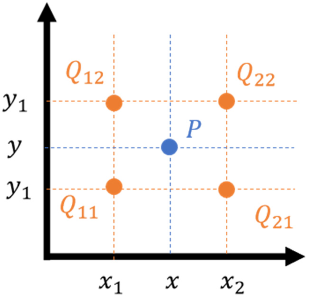
Bilinear interpolation achieves a continuous smooth interpolation effect by local linear weighting [18]. In this study, the parameterization of bilinear interpolation was implemented directly using Equation (2).

$$f\left(x,y\right)={\displaystyle \frac{y_2-y}{y_2-y_1}}f\left(x,y_1\right)+{\displaystyle \frac{y-y_1}{y_2-y_1}}f\left(x,y_2\right)$$

(2)

If we want to find the value of the unknown function P at the point (x, y), suppose we know the values of P at four points Q₁₁ = (x₁, y₁), Q₁₂ = (x₁, y₂), Q₂₁ = (x₂, y₁), and Q₂₂ = (x₂, y₂) (as in Figure 2) [19]. And the parameters f (x, y₁) and f (x, y₂) of Equation (2) are calculated from Equations (3) and (4).

$$f\left(x,y_1\right)={\displaystyle \frac{x_2-x}{x_2-x_1}}f\left(Q_{11}\right)+{\displaystyle \frac{x-x_1}{x_2-x_1}}f\left(Q_{21}\right)$$

(3)

$$f\left(x,y_2\right)={\displaystyle \frac{x_2-x}{x_2-x_1}}f\left(Q_{12}\right)+{\displaystyle \frac{x-x_1}{x_2-x_1}}f\left(Q_{22}\right)$$

(4)

The method finally generates a continuously differentiable interpolated surface. It is computationally efficient and can suppress the jagged effect, but it may blur the high-frequency details and is suitable for natural image resampling or continuous physical field reconstruction [20].

Cubic spline interpolation is an efficient smooth interpolation method for one-dimensional data [21], and it can also be extended to 2D data like the method of bilinear interpolation described above. Its core idea is to divide the interval between data points into several small segments and construct an independent cubic polynomial function on each small segment, so that the adjacent segments not only have continuous function values at the connection point (i.e., the original data points), but also ensure the continuity of the first-order and second-order derivatives [22].

The advantage of cubic spline interpolation lies in its smoothness and localization, and it is widely used in fields that require high-precision smoothing of curves, such as contouring in mechanical engineering, time-series analysis of financial data, generation of motion paths in animation, and fitting processing of scientific experimental data [23].

3.2. Model Architectural Design

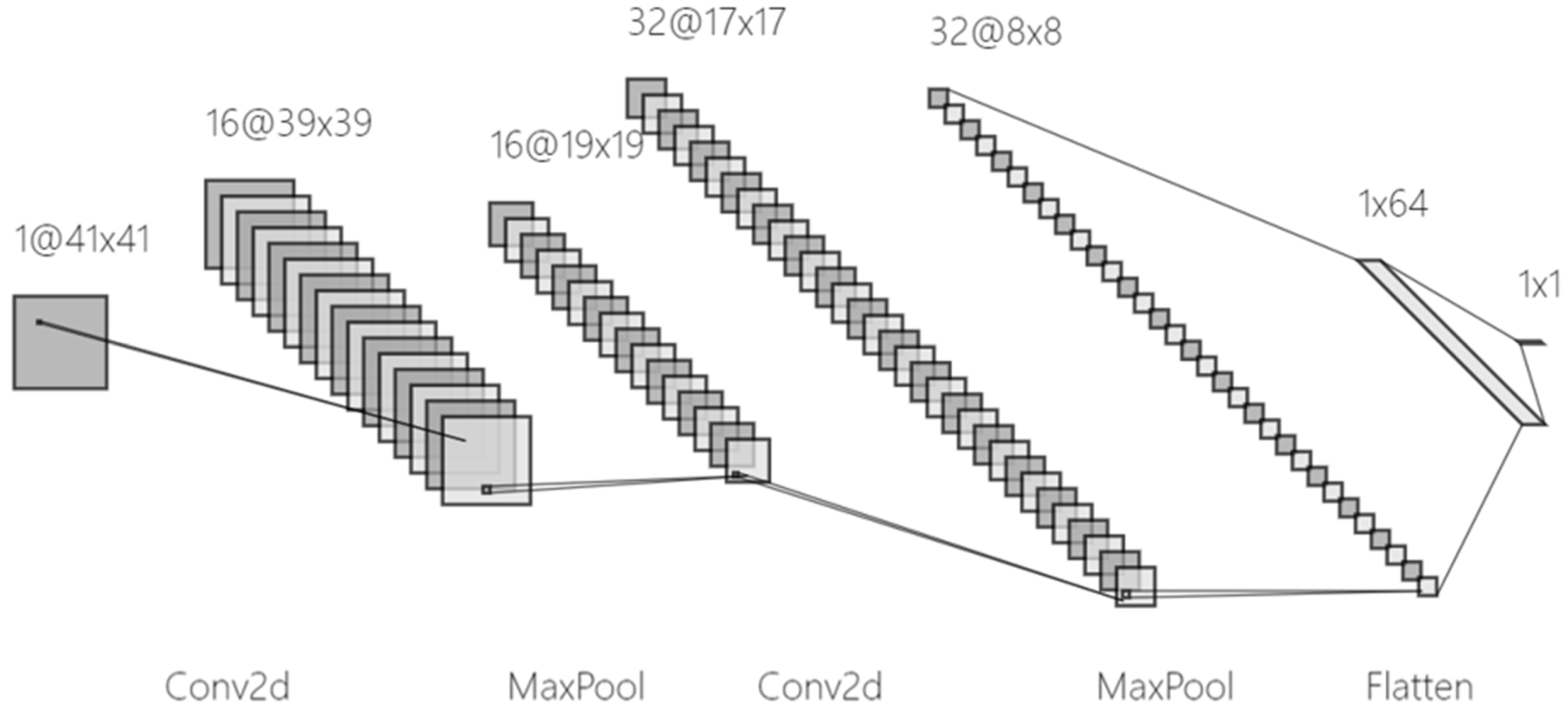
In this study, a lightweight convolutional neural network is proposed for the spatial properties of ERA5 reanalysis data, with model training and testing conducted on the Colab T4 GPU (Google Colab, Google, Mountain View, CA, USA).

The model input is a 41 × 41 temperature matrix which represents the study area of 17–27° N and 109–119° E. Our model utilizes two layers of convolution and pooling to extract features (as shown in Figure 3), after which the grid data values of Macau are extracted by fully connected layers. During training under mean square error loss function, the regularization strategies of batch normalization (BN) and a 0.2 dropout are used to prevent overfitting of high-dimensional features.

Dropout is more widely used in image tasks, but it is less used in regression tasks. This study is a regression task based on image-like two-dimensional grid data, which combines the characteristics of image task and regression task, so BN (batch normalization) and dropout are still effective in preventing overfitting in this regression task model. In the image task, the pooling layer is used to extract features and prevent overfitting. In this study, pooling can extract features from 2D grid data, reduce the number of parameters, and prevent overfitting in subsequent regression tasks. Overall, the addition of dropout and pooling leads to better model performance in this type of regression task with image input.

3.3. Model Evaluation Criteria

Mean square error (MSE), Root Mean Square Error (RMSE), Mean Absolute Error (MAE), Mean Relative Error (MRE), and Pearson correlation coefficient are commonly used evaluation metrics for forecasting tasks, which describe the gap between actual and predicted values. In this study, these five metrics will be used to compare the performance of the models [24].

MSE is a widely used measure of model prediction accuracy in regression analysis [25]. It quantifies the degree of model fit by calculating the average of the squares of the errors between the predicted and true values, and the MSE is calculated as follows:

$$MSE={\displaystyle \frac{1}{n}}\sum _{i=1}^n{\left(y_i-\widehat{y_i}\right)}^2$$

(5)

Specifically, for a dataset containing n samples, let y_i be the true value of the i-th sample and $\widehat{y_i}$ be the corresponding predicted value.

The MSE gives a higher weight to larger errors because the errors are squared during the calculation. This makes the MSE more sensitive to outliers, and a large prediction error can significantly increase the value of the MSE [26]. Therefore, the MSE can effectively reflect the overall error of the model but may exaggerate the inaccuracy of the model in datasets where outliers are present [27].

The RMSE is the square root of the MSE and is also used to assess the predictive performance of regression models [28]. It is closely related to the MSE but has the same magnitude as the original data, making it more intuitive in interpreting model errors. The RMSE is calculated as follows:

$$RMSE=\sqrt{{\displaystyle \frac{1}{n}}\sum _{i=1}^n{\left(y_i-\widehat{y_i}\right)}^2}$$

(6)

The RMSE combines the prediction errors of all samples, and it is able to balance the effects of different sample errors due to the squaring and squaring operations performed on the errors. Similar to MSE, RMSE is sensitive to larger errors, but it more directly reflects the average degree of deviation between the model’s predicted and true values [29]. In practice, the smaller the RMSE, the higher the predictive accuracy of the model [30].

MAE is another commonly used regression model assessment metric, which measures the predictive accuracy of a model by calculating the average of the absolute errors between the predicted and true values [31]. For a given dataset, the MAE is calculated as follows:

$$MAE={\displaystyle \frac{1}{n}}\sum _{i=1}^n\left|y_i-\widehat{y_i}\right|$$

(7)

Unlike MSE and RMSE, MAE treats all errors equally and does not consider the direction of the error but only focuses on the magnitude of the error [26]. This makes the MAE relatively less sensitive to outliers and more robust to the average prediction error of the model [32].

MRE is a statistical metric used to measure the relative error between the predicted or estimated value and the true value [33]. In many fields such as data analytics, machine learning, engineering, etc., MRE is a useful metric when it is necessary to assess the accuracy of model prediction results or estimation methods. It can reflect the degree of deviation of the predicted value relative to the true value, and MRE is more concerned with the proportion of the error in the true value than MAE [34].

$$MRE={\displaystyle \frac{1}{n}}\sum _{i=1}^n\left|{\displaystyle \frac{\widehat{y_i}-y_i}{y_i}}\right|$$

(8)

The Pearson correlation coefficient is a statistical measure of the strength and direction of the linear relationship between two continuous variables, taking values in the range [−1, 1]. In machine learning, it is commonly used to assess the trend consistency between the predicted and true values of a regression model [35].

$$r={\displaystyle \frac{{\sum }_{i=1}^n\left(x_i-\overline{x}\right)\left(y_i-\overline{y}\right)}{\sqrt{{\sum }_{i=1}^n{\left(x_i-\overline{x}\right)}^2}\sqrt{{\sum }_{i=1}^n{\left(y_i-\overline{y}\right)}^2}}}$$

(9)

4. Experimental Results and Discussion

In this experiment, a regional temperature downscaling model is constructed based on a convolutional neural network, with the input being a 41 × 41 matrix of ERA5 reanalysis data temperature field at T moments, and the output is the observed temperature of Macau stations at the corresponding moments. Ground-based observations from the Macau Meteorological Bureau were used as the true value comparison, and the evaluation metrics included RMSE, MSE, MAE, MRE, and Correlation.

4.1. Temperature Interpolation for Macau Stations Based on CNN Modeling

From the evaluation metrics (

Table 1. Comparison of nearest-neighbor interpolation, bilinear interpolation, cubic spline interpolation, and deep learning methods.

Methods	RMSE	MSE	MAE	MRE (%)	Correlation
Nearest	1.175	1.381	0.944	4.401	0.983
Linear	1.315	1.730	1.073	5.250	0.977
Cubic	1.334	1.779	1.087	5.308	0.975
Ours	0.924	0.854	0.685	0.530	0.986

), the model prediction shows significant advantages in the immediate prediction (0 h) scenario. Compared with the traditional interpolation methods Nearest, Linear, and Cubic, the RMSE of the model prediction is only 0.924, which is reduced by 21.4%, 30.7%, and 30.7% compared to Nearest, Linear, and Cubic, respectively; the MAE is 0.685, which is reduced by 27.4%, 37.0%, and 37.7%; the MRE is as low as 0.530%, while the MRE of the traditional method is between 4.401 and 5.308%; the MSE is 0.854, which is much lower than that of the traditional method, which is between 1.381 and 1.779; the correlation coefficient is as high as 0.986, which indicates that the model is able to accurately capture more than 99% of data fluctuation pattern, far more than the 0.975–0.983 of the traditional method.

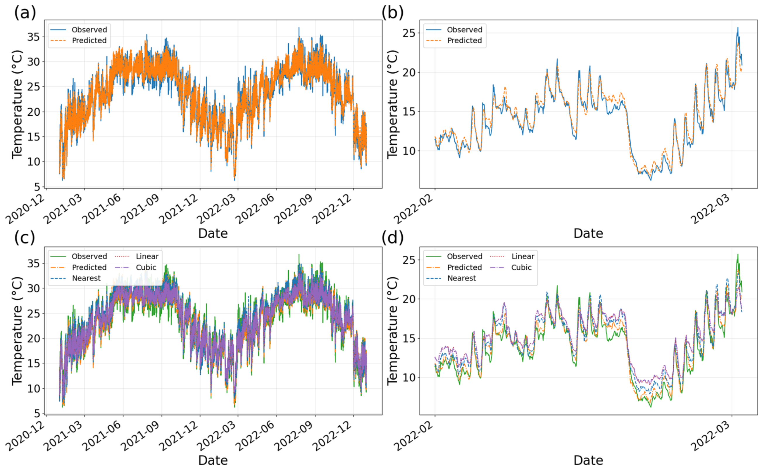
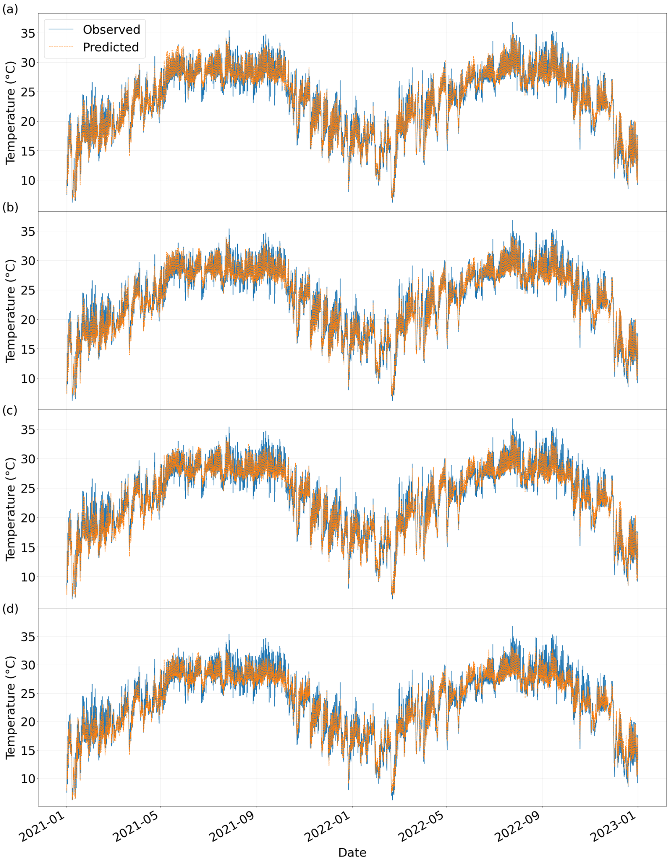
The comparative time-series plot of temperature forecasts constructed in this study (Figure 4) clearly presents the dynamic matching relationship between the model predictions and the actual observations. The horizontal axis of the time series plot covers the complete observation period from 1 January 2021 to 1 January 2023 (with a time resolution of 1 h), and the vertical axis shows the temperature range from 5 °C to 35 °C. The blue solid line represents the actual temperature profile, and the orange dashed line represents the model prediction. The solid blue line represents the actual observed temperature profile and the dashed orange line represents the model prediction, and the two trends are highly coincident (Correlation r = 0.986), indicating that the model is able to effectively capture the core pattern of diurnal temperature fluctuations and sudden weather events.

4.2. Temperature Prediction for Macau Stations Based on CNN Models

The longitudinal comparative analysis of the model performance under different prediction time frames shows (

Table 2. Comparison of deep learning models for temperature prediction in Macau with 0–3 h lead times using ERA5 reanalysis data.

Lead Time	RMSE	RMSE Growth Rate	MAE	MRE (%)	Correlation
0 h	0.924	-	0.685	0.530	0.986
+1 h	1.026	+11.0%	0.756	0.588	0.983
+2 h	1.131	+22.4%	0.831	0.653	0.979
+3 h	1.260	+36.4%	0.944	0.725	0.974

) that the model error increases with the prolongation of prediction time. The RMSE, MAE, and MRE all show an increasing trend, with the RMSE increasing by 0.112 per hour on average, which is in line with the law of accumulation of meteorological prediction errors, indicating that the uncertainty of the model prediction increases with the increase in time span.

Despite the rise in error, the model correlation shows a stable performance. The correlation coefficient decays from 0.986 to 0.974 from the current moment to the next 3 h prediction time, but it still outperforms some of the traditional interpolation methods, indicating that the model is able to capture the intrinsic correlation of the data better, even in long-time prediction.

Combined with its unique advantage in predicting the future time period and its comprehensive performance in error control and correlation retention, the model has high practical value in the fields of meteorological prediction and geo-environmental analysis and can provide valuable reference for related work.

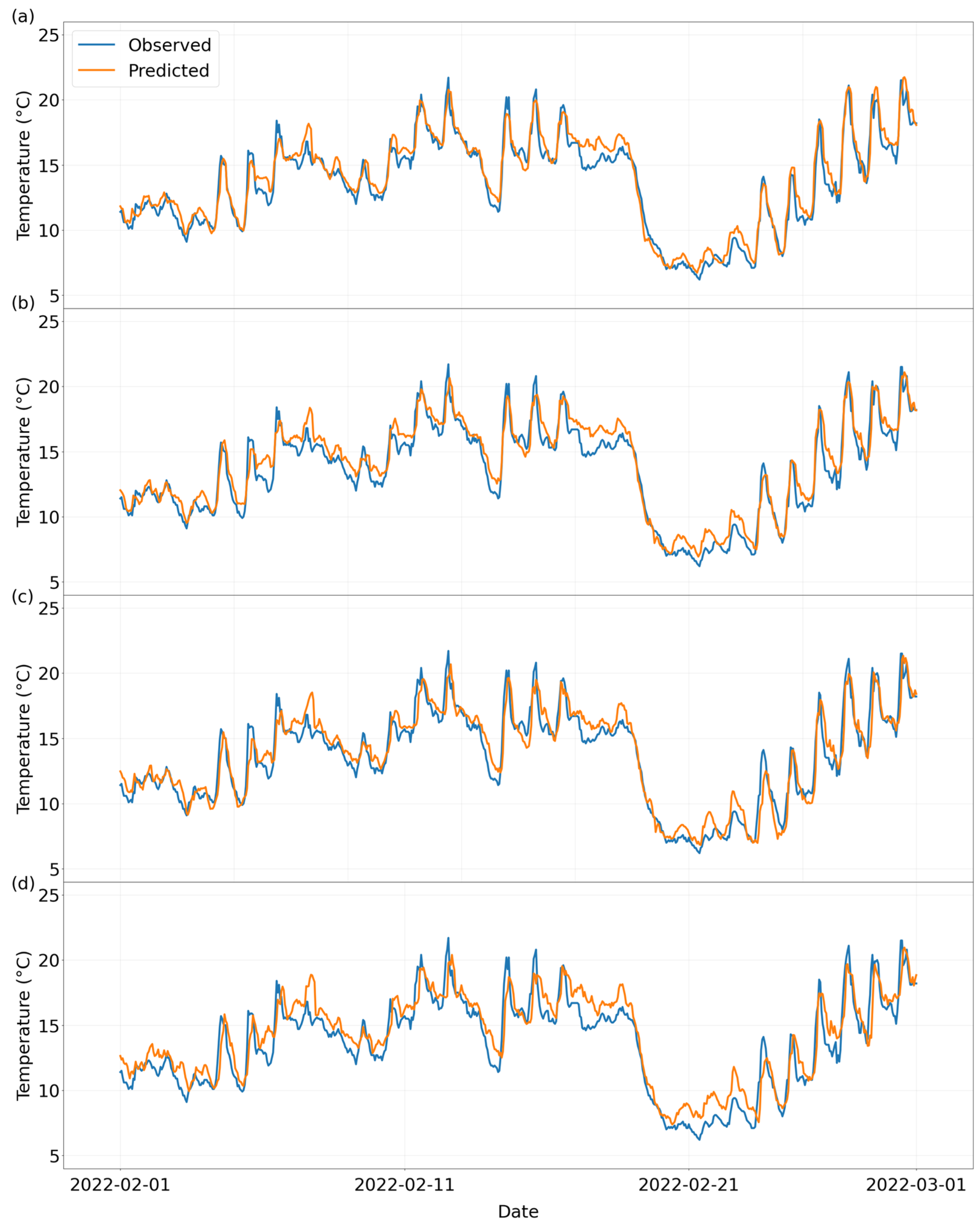
In the time-series analysis section, the decay pattern of prediction accuracy with the prediction step size is systematically revealed by constructing the 0–3 h time scale prediction comparison graph (Figure 5 and Figure 6). The model fitting effect is significantly better than that of the traditional interpolation method, and the prediction curves are highly consistent with the measured temperature trends: whether it is the long-term trend prediction over a two-year time span or the short-term fluctuation simulation over a three-month time window, the key features of the temperature changes can be effectively captured.

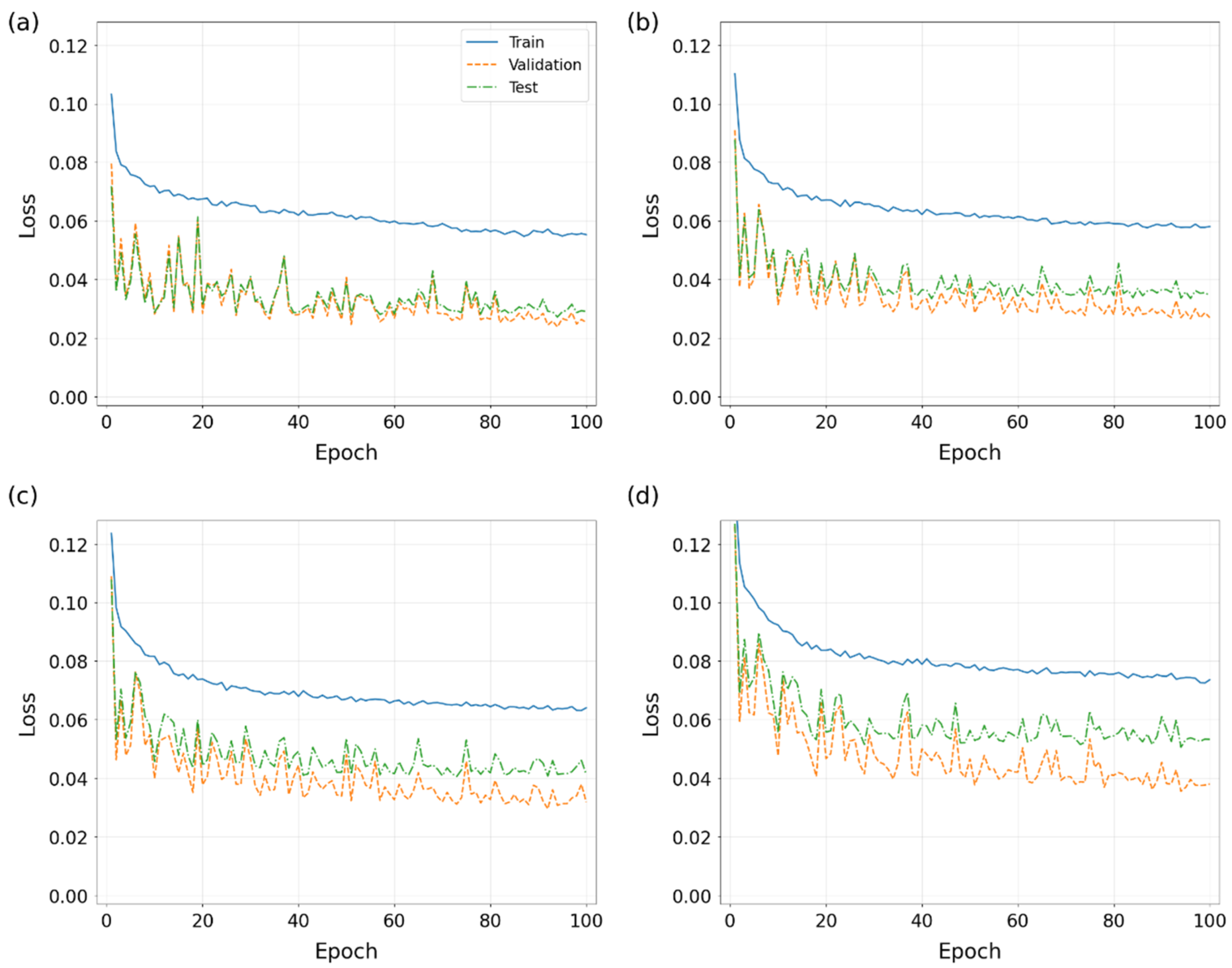
Figure 7 shows that the training loss is larger than the validation and test losses. This is because the training loss includes the errors from model and dropout, whereas in validation and test modes, the loss only reflects the model errors without dropout. On the other hand, the validation and test losses are gradually separated as the prediction time step continues to increase. This phenomenon implies that the difference between the model’s performance on the validation and test sets gradually increases as the prediction time span increases. The reason for this may be that the uncertainty and complexity in the data increase significantly as the prediction time span expands, and although the model learns on the training set, its generalization ability is challenged in the face of the diverse data characteristics of the validation set and the test set in long time scales.

4.3. Discussions

In an in-depth investigation of the model performance for different prediction timings, this study clearly reveals the superiority of the CNN model over the traditional bilinear interpolation and other methods. In terms of error indicators, the RMSE, MAE, and MRE of the DL model are significantly lower than those of the traditional method in the instantaneous prediction (0 h), and with the extension of the prediction time to the next three hours, although the error increases, the error growth rate and the final absolute value of the error are still in the acceptable range, and the correlation coefficient is always maintained at a high level, which is better than that of the traditional bilinear interpolation method. This indicates that the CNN model has an excellent ability to capture the data fluctuation patterns and control the error accumulation.

Given the excellent performance of the CNN model in the region around Macau, it is feasible and potentially valuable to generalize it to other regions. The error growth pattern over time is in line with the general characteristics of meteorological forecasts and maintains good correlation under long time forecasts, which provides a solid theoretical basis for its application in different geographic environments. Although there are geographical differences in different regions, the principles of spatial and temporal changes in meteorological elements are common, and the powerful learning and adaptation ability of the CNN model means it is expected to realize accurate weather prediction and geographic environment analysis in other regions as well.

5. Conclusions

In this study, a lightweight temperature downscaling model with a two-layer CNN structure is used to achieve accurate prediction of the observed temperature at a single station in Macau from ERA5 reanalysis data.

The experimental results show that our model is far better than the traditional interpolation method in the instantaneous prediction (0 h); the RMSE of the model is 21% lower than that of Nearest interpolation and 31% lower than that of Linear and Cubic interpolation. Our model’s stability is especially outstanding in multi-temporal prediction, and the RMSE of the next 3 h (+3 h) prediction is still better than the instantaneous results of all the interpolation methods, with the correlation coefficients of all the time periods higher than 0.97. Moreover, the error increases with the increase in prediction step, which is in line with the law of meteorological prediction.

The excellent performance of this model provides a more reliable and accurate prediction tool for climate research, ecological environment monitoring, and other fields, and strongly promotes the research progress and practical application of related fields in a wider scope. In view of its excellent results in the region around Macau and the universality of the principle of spatial and temporal variations in meteorological elements, the model is expected to be extended to other regions, providing solid data support and technical guarantee for cross-regional decision-making and environmental management, and has a broad application prospect in future meteorological and geo-environmental studies.

References

- Shu, H.; Wang, Y.; Song, W.; Guo, H.; Song, Z. Forecasting the Future with Future Technologies: Advancements in Large Meteorological Models. arXiv 2024, arXiv:2404.06668. [Google Scholar]
- Ramage, C.S. Forecasting in meteorology. Bull. Am. Meteorol. Soc. 1993, 74, 1863–1872. [Google Scholar] [CrossRef]
- Mu, M.; Chen, B. Methods and uncertainties of meteorological forecast. Meteorol. Mon. 2011, 37, 1–13. [Google Scholar]
- Jiang, Y.; Yang, K.; Shao, C.; Zhou, X.; Zhao, L.; Chen, Y.; Wu, H. A downscaling approach for constructing high-resolution precipitation dataset over the Tibetan Plateau from ERA5 reanalysis. Atmos. Res. 2021, 256, 105574. [Google Scholar] [CrossRef]
- Li, Z.; Liu, F.; Yang, W.; Peng, S.; Zhou, J. A survey of convolutional neural networks: Analysis, applications, and prospects. IEEE Trans. Neural Netw. Learn. Syst. 2021, 33, 6999–7019. [Google Scholar] [CrossRef]
- Alzubaidi, L.; Zhang, J.; Humaidi, A.J.; Al-Dujaili, A.; Duan, Y.; Al-Shamma, O.; Santamaría, J.; Fadhel, M.A.; Al-Amidie, M.; Farhan, L. Review of deep learning: Concepts, CNN architectures, challenges, applications, future directions. J. Big Data 2021, 8, 53. [Google Scholar] [CrossRef]
- Bhatt, D.; Patel, C.; Talsania, H.; Patel, J.; Vaghela, R.; Pandya, S.; Modi, K.; Ghayvat, H. CNN variants for computer vision: History, architecture, application, challenges and future scope. Electronics 2021, 10, 2470. [Google Scholar] [CrossRef]
- Kattenborn, T.; Leitloff, J.; Schiefer, F.; Hinz, S. Review on Convolutional Neural Networks (CNN) in vegetation remote sensing. ISPRS J. Photogramm. Remote Sens. 2021, 173, 24–49. [Google Scholar] [CrossRef]
- Lam, N.S.N. Spatial interpolation methods: A review. Am. Cartogr. 1983, 10, 129–150. [Google Scholar] [CrossRef]
- Hersbach, H.; Bell, B.; Berrisford, P.; Hirahara, S.; Horányi, A.; Muñoz-Sabater, J.; Nicolas, J.P.; Peubey, C.; Radu, R.; Schepers, D.; et al. The ERA5 global reanalysis. Q. J. R. Meteorol. Soc. 2020, 146, 1999–2049. [Google Scholar] [CrossRef]
- Cucchi, M.; Weedon, G.P.; Amici, A.; Bellouin, N.; Lange, S.; Schmied, H.M.; Hersbach, H.; Buontempo, C. WFDE5: Bias adjusted ERA5 reanalysis data for impact studies. Earth Syst. Sci. Data Discuss. 2020, 2020, 2097–2120. [Google Scholar] [CrossRef]
- Xu, J.; Ma, Z.; Yan, S.; Peng, J. Do ERA5 and ERA5-land precipitation estimates outperform satellite-based precipitation products? A comprehensive comparison between state-of-the-art model-based and satellite-based precipitation products over mainland China. J. Hydrol. 2022, 605, 127353. [Google Scholar] [CrossRef]
- Mangum, B.W.; Furukawa, G.T.; Kreider, K.G.; Meyer, C.W.; Ripple, D.C.; Strouse, G.F.; Tew, W.L.; Moldover, M.R.; Carol Johnson, B.; Yoon, H.W.; et al. The Kelvin and temperature measurements. J. Res. Natl. Inst. Stand. Technol. 2001, 106, 105. [Google Scholar] [CrossRef]
- Caruso, C.; Quarta, F. Interpolation methods comparison. Comput. Math. Appl. 1998, 35, 109–126. [Google Scholar] [CrossRef]
- Li, X.; Cheng, G.; Lu, L. Comparison of spatial interpolation methods. Adv. Earth Sci. 2000, 15, 260–265. [Google Scholar]
- Rukundo, O.; Cao, H. Nearest neighbor value interpolation. arXiv 2012, arXiv:1211.1768. [Google Scholar]
- Xing, Y.; Song, Q.; Cheng, G. Benefit of interpolation in nearest neighbor algorithms. SIAM J. Math. Data Sci. 2022, 4, 935–956. [Google Scholar] [CrossRef]
- Kirkland, E.J.; Kirkland, E.J. Bilinear interpolation. In Advanced Computing in Electron Microscopy; Springer: New York, NY, USA, 2010; pp. 261–263. [Google Scholar]
- Monasse, P. Extraction of the level lines of a bilinear image. Image Process. Line 2019, 9, 205–219. [Google Scholar] [CrossRef]
- Smith, P.R. Bilinear interpolation of digital images. Ultramicroscopy 1981, 6, 201–204. [Google Scholar] [CrossRef]
- McKinley, S.; Levine, M. Cubic spline interpolation. Coll. Redw. 1998, 45, 1049–1060. [Google Scholar]
- Wolberg, G. Cubic Spline Interpolation: A Review; Columbia University: New York, NY, USA, 1988. [Google Scholar]
- Hou, H.; Andrews, H. Cubic splines for image interpolation and digital filtering. IEEE Trans. Acoust. Speech Signal Process. 1978, 26, 508–517. [Google Scholar]
- Chicco, D.; Warrens, M.J.; Jurman, G. The coefficient of determination R-squared is more informative than SMAPE, MAE, MAPE, MSE and RMSE in regression analysis evaluation. Peerj Comput. Sci. 2021, 7, e623. [Google Scholar] [CrossRef]
- Schluchter, M.D. Mean square error. In Encyclopedia of Biostatistics; Wiley: New York, NY, USA, 2005; p. 5. [Google Scholar]
- Hodson, T.O. Root mean square error (RMSE) or mean absolute error (MAE): When to use them or not. Geosci. Model. Dev. Discuss. 2022, 15, 5481–5487. [Google Scholar] [CrossRef]
- Wang, Z.; Bovik, A.C. Mean squared error: Love it or leave it? A new look at signal fidelity measures. IEEE Signal Process. Mag. 2009, 26, 98–117. [Google Scholar] [CrossRef]
- Chai, T. Root Mean Square. In Encyclopedia of Mathematical Geosciences; Springer International Publishing: Cham, Switzerland, 2023; pp. 1236–1238. [Google Scholar]
- Kamble, V.B.; Deshmukh, S.N. Comparision between accuracy and MSE, RMSE by using proposed method with imputation technique. Orient. J. Comput. Sci. Technol. 2017, 10, 773–779. [Google Scholar] [CrossRef]
- Mentaschi, L.; Besio, G.; Cassola, F.; Mazzino, A. Problems in RMSE-based wave model validations. Ocean. Model. 2013, 72, 53–58. [Google Scholar] [CrossRef]
- Wang, W.; Lu, Y. Analysis of the mean absolute error (MAE) and the root mean square error (RMSE) in assessing rounding model. In IOP Conference Series: Materials Science and Engineering; IOP Publishing: Bristol, UK, 2018; Volume 324, p. 012049. [Google Scholar]
- Willmott, C.J.; Matsuura, K. Advantages of the mean absolute error (MAE) over the root mean square error (RMSE) in assessing average model performance. Clim. Res. 2005, 30, 79–82. [Google Scholar] [CrossRef]
- Foss, T.; Myrtveit, I.; Stensrud, E. MRE and heteroscedasticity: An empirical validation of the assumption of homoscedasticity of the magnitude of relative error. In Proceedings of the ESCOM, 12th European Software Control and Metrics Conference, Munich, Germany, 18–20 April 2000; pp. 157–164. [Google Scholar]
- Yang, Y.; Ye, F. General relative error criterion and M-estimation. Front. Math. China 2013, 8, 695–715. [Google Scholar] [CrossRef]
- Cohen, I.; Huang, Y.; Chen, J.; Benesty, J. Pearson correlation coefficient. In Noise Reduction in Speech Processing; Springer: Berlin/Heidelberg, Germany, 2009; pp. 1–4. [Google Scholar]