Reliability Assessment of Ship Lubricating Oil Systems Through Improved Dynamic Bayesian Networks and Multi-Source Data Fusion

Abstract

The operational efficiency and reliability of the ship’s lubrication oil system directly impact the vessel’s safety. Traditional reliability analysis methods struggle to effectively handle the system’s dynamic characteristics and multi-source data analysis. To address these issues, this study proposes an innovative method that integrates feature dimensionality reduction, a dynamic Bayesian network of gravity model to improve the accuracy of system reliability analysis. First, the proportional hazards model is used to evaluate the operational reliability of each component, providing a quantitative basis for assessing the system’s health status through failure rate estimation. Then, a dynamic Bayesian network model is employed for overall system reliability analysis, fully considering the impact of multi-state devices and different maintenance strategies. The proposed DBN-based reliability assessment method achieves significant improvements over the traditional Fault Tree Analysis (FTA). The reliability of the main lubrication oil system (GUB) increases from 0.169 to 0.261, representing a 9.2% improvement; under scheduled maintenance conditions, the system reliability stabilizes at approximately 0.9873 after $0.4\times {10}^5$ h, compared to only 0.24 without maintenance. The proposed method effectively evaluates the reliability of the lubrication oil system, and the maintenance strategy using this method can greatly improve the reliability, providing strong support for scientifically guiding maintenance decisions.

1. Introduction

1.1. Background and Rationale

As a critical subsystem of the ship’s main engine and auxiliary machinery, the lubrication system directly impacts the smooth operation of the ship. According to statistics from the European Maritime Safety Agency (EMSA), accidents caused by lubrication system failures represent a significant portion of engine-related failures, severely affecting operational efficiency and safety [1]. Due to the complex operating environment of ships, the lubrication system is subjected to high temperatures, high pressures, and prolonged exposure to marine corrosion, making it vulnerable to wear, degradation, and sudden failures. The International Safety Management (ISM) Code, established by the International Maritime Organization (IMO), requires ship operators to develop maintenance systems and implement maintenance plans aimed at reducing lubrication system failures and ensuring stable operations [2]. Therefore, conducting a reliability analysis of the ship’s lubrication oil system is essential.

1.2. Literature Review

Early research on ship system reliability analysis primarily relied on the binary state concept, where the system was either in normal operation or in a failure state [3]. Common methods, such as Fault Tree Analysis (FTA) and reliability block diagram (RBD), were used to assess the reliability of ship systems, providing valuable insights for system design and fault detection [4]. Since equipment often operates under various states, such as degraded or failure states, the binary state model cannot accurately represent the evolution of equipment reliability [5]. As a result, some scholars have adopted methods like Markov models and Generalized Generating Functions (GGFs) to assess the reliability of multi-state ship systems [6]. However, these methods have their limitations. For instance, the Markov method faces the issue of state explosion when analyzing multi-state systems with numerous components [7].

To address these issues, Bayesian networks (BNs) have been applied to the reliability analysis of lubrication systems. Ait Allal et al. [8] used Bayesian network modeling to identify weak links and propose improvements, but their inference relied on preset data, lacking real-time capabilities. Zhao et al. [9] combined Fault Tree Analysis (FTA) and BN to analyze the ship lubrication system, identifying key components and recommending backup monitoring, but their analysis was limited to the design phase. It could not achieve real-time inference. With the increasing complexity of industrial equipment, static Bayesian analysis methods struggle to meet the demands of real-time health monitoring. As an extension of Bayesian networks, Dynamic Bayesian Networks (DBNs) can process time-series data and capture dynamic changes in systems. DBNs not only inherit the advantages of Bayesian networks in handling uncertainty but also reduce the number of conditional probability table parameters compared to Markov models, addressing some of the state explosion issues and making them suitable for complex reliability evaluation systems [10]. Additionally, the root nodes in DBNs can be divided into multi-state nodes, which effectively describe the fault evolution of multi-state equipment and analyze the impact of different maintenance strategies on system reliability. Currently, DBN-based reliability analysis methods are widely applied in complex systems, such as train control systems and underwater drilling trees, showing promising evaluation results [11]. Li et al. [12] proposed a method for converting dynamic reliability block diagrams (DRBDs) into DBNs, demonstrating their efficient analysis capabilities for large-scale critical systems. Gao et al. [13] developed a DBN-based intelligent factory health assessment model, showing excellent performance in equipment health-level prediction.

In recent years, multidimensional data analysis techniques have demonstrated significant advantages in information fusion, fault pattern recognition, and condition assessment within the field of complex system fault diagnosis. Jiang et al. [14] proposed a multi-channel tensor fusion method, highlighting the strong coupling characteristics among multi-channel sensors—such as temperature, pressure, and oil quality analysis—in marine lubricating oil systems. Tensor-based modeling can more effectively capture high order features of system operating states, providing a feasible basis for fault identification in subsequent reliability evaluations by enabling the use of high dimensional classifiers such as tensor machines. Xu et al. [15] developed an expert system for power transformer fault diagnosis based on multidimensional data fusion and factor analysis. This system achieves data fusion at the decision level and employs factor analysis to calculate fusion weights, thereby improving diagnostic accuracy. The approach was validated on a 110 kV transformer. Orošnjak et al. [16] analyzed maintenance practice data from 115 enterprises using hydraulic systems by employing machine learning models such as KNN, Ridge, and SVR. Through model agnostic feature importance analysis, they identified variables with significant impacts on system availability and sustainability and further established a hypothesis testing mechanism to interpret the roles of these variables. This study emphasizes the importance of interpreting variable contributions within multidimensional data, which is particularly critical for multi-source data modeling in marine lubricating oil systems, due to the large number of variables and high data noise. Multidimensional data analysis is central to robust fault diagnosis and reliability evaluation, laying a solid foundation for advancing dynamic Bayesian network methodologies.

Selecting feature parameters from the signals of the ship’s lubrication system is crucial for conducting reliability analysis. Zhengjia He et al. [17] proposed a method for operational reliability assessment based on the operational state information of mechanical equipment. They established a mapping relationship between equipment operational state information and reliability, calculated operational reliability, and introduced a reliability assessment method for equipment operation under small sample conditions, using normalized wavelet information entropy and damage quantification for identification. Guangyao Ouyang et al. [18] proposed a second-order model analysis method, performing finite element analysis on a local model with boundary conditions derived from overall calculations, and conducted a reliability analysis for high-speed, high-power diesel engines. Chunwei Zhu et al. [19] established a relevant prediction model using a Markov chain based on gear transmission data, and employed mathematical methods to predict the reliability of gear transmissions. Congcong Zhao [20] utilized a local cutspace arrangement algorithm to reduce the dimensionality of high-dimensional feature vectors extracted from vibration signals. They then applied a chaotic particle swarm optimization algorithm to estimate parameters for the proportional hazards model (PHM), completing a reliability analysis for structural components of train drive systems. Lang Cao et al. [21] determined the feature parameter set required for reliability analysis of gearbox performance degradation through experimental verification. Duan et al. [22] extracted distance evaluation factor values from the frequency band energy using wavelet packet analysis, and used these as response covariates for the Weibull proportional hazards model in gear reliability assessment. Sun et al. [23] applied distance evaluation methods for dimensionality reduction on bearing fault data, achieving objective identification of fault feature parameters for bearing fault recognition. Lu et al. [24] introduced a new fault feature extraction method for rotating machinery based on adaptive multi-wavelet and distance evaluation indices, improving fault diagnosis accuracy. Selecting feature parameters from the signals of the ship’s lubrication system is crucial for conducting reliability analysis. Single feature parameters are insufficient to reflect the overall degradation characteristics of the lubrication system, while an excessive number of parameters can affect the efficiency of subsequent reliability analysis. Existing dynamic Bayesian theory faces challenges in accurately reflecting the system’s actual operating conditions when analyzing multi-sensor parameters of the lubrication system [25].

1.3. Aims and Objectives

In the modern ship power system, the lubricating oil system is a key subsystem to ensure the stable operation of the main engine and auxiliary equipment, and its reliability is directly related to the operation safety and life of the ship equipment. However, due to the ship lubrication system usually operating in strong interference, high load, and variable operating conditions, its complex structure includes multiple types of key components and a large amount of sensor data, which makes the traditional reliability assessment methods face many challenges in dealing with dynamic degradation, multi-source data fusion, and complex dependence between states. The traditional static model cannot reflect the dynamic evolution process of the system running state, and the simple threshold judgment cannot effectively deal with the noise, uncertainty, and fuzzy boundary in the signal. In addition, the existing methods strongly rely on expert experience for state recognition and health assessment, and lack scalable and data-driven modeling mechanisms, which are difficult to adapt to the increasing needs of the intelligent operation and maintenance of ship equipment.

In order to solve the above problems, this paper aims to construct a reliability evaluation method of marine lubricating oil systems based on an improved dynamic Bayesian network and multi-source data fusion. From system modeling, signal processing, feature extraction, state recognition, probabilistic modeling to system level reasoning, a whole process method framework running through the data layer and decision layer is proposed. The goal of this study is to achieve the accurate identification of the lubricating oil system operating state, dynamic reliability prediction, and operation and maintenance strategy optimization. The experimental results show that the proposed method not only has good accuracy in instantaneous availability evaluation but also shows strong scalability and practicability in multi-state complex systems, which provides reliable data support and decision-making basis for the health management and fault prevention of ship critical systems. Finally, this paper hopes to promote the traditional reliability analysis from static modeling to dynamic, data-driven, and intelligent direction, and provide theoretical basis and engineering practice value for the efficient and safe operation of ship equipment.

Focusing on the reliability evaluation problem of marine lubricating oil systems in a complex operation environment, this study proposes a multi-level analysis method that integrates multi-source signal processing, feature dimension reduction, and a dynamic Bayesian Network (DBN) enhancement mechanism, and constructs a dynamic reliability modeling framework from equipment level to system level. This paper aims to realize the accurate identification, health assessment, and maintenance decision support of a lubrication system.

In the second part, the Methodology, the simulation model of the lubricating oil system is constructed by AMESim software 2021.1, the EEMD algorithm is used to denoise the multi-source sensor signals, and the nonlinear time-varying features are extracted by combining wavelet packet analysis, and the automatic identification of the operation state is realized based on K-means clustering. In the aspect of system reliability modeling, a Dynamic Bayesian Network (DBN) based on a fault tree structure was constructed to quantify the probability transition relationship of equipment state evolution over time, and distinguish the state transition rate under the situation with and without maintenance. Furthermore, the proportional hazards model (PHM) is integrated to model the independent life of each key component, and the optimal failure distribution (Weibull, exponential, or normal) is selected according to the historical life data.

In the third chapter, the experimental verification part takes a certain type of diesel engine lubricating oil system as the object, and verifies the accuracy and effectiveness of the proposed method in state discrimination, feature sensitivity assessment, and system availability prediction through sensor-measured data and simulation results. It effectively verifies the engineering applicability of the proposed method under multi-state equipment and complex maintenance strategies. Sensitivity analysis further identifies high-impact components such as electric pumps and turbopumps to provide a quantitative basis for priority maintenance. The high consistency with the traditional reliability block diagram and Monte Carlo simulation results also confirms the effectiveness of the proposed method.

Chapter 4, the Conclusion section, summarizes the innovative results of this research in high-dimensional feature dimensionality reduction, dynamic state recognition, multi-state probabilistic modeling, and system usability evaluation. The research shows that periodic maintenance can significantly improve system reliability, which verifies the advantages of the DBN model in multi-state system modeling. At the same time, it is pointed out that the current model still needs to be optimized in the face of more complex environmental disturbances, sensor failures or missing data. In the future, the combination of digital twin, the intelligent optimization algorithm, and multimodal fusion technology will be explored to further realize the whole life cycle intelligent health management of ship key systems.

2. Methodology

2.1. Lubrication System Simulation and Component Introduction

By calculating the distance evaluation factors of various feature parameters, the standard deviation and absolute mean value of the fluctuation signal were selected as the time-domain feature parameters to be used as response covariates in the Weibull proportional hazards model [26]. The lubrication oil system plays a crucial role in diesel engines, effectively reducing friction and wear while extending the machine’s service life. It is particularly suitable for large machinery, such as marine engines [27]. In this study, the Chinese Zibo Power Co., Ltd.’s 6210ZLC/S-2 diesel engine lubrication oil system was selected as the target system for reliability assessment, as shown in Figure 1. A simulation analysis was conducted using the operating time and maintenance strategy of the diesel engine system. The lubrication oil system operates under normal conditions for approximately 29% of the year and undergoes scheduled maintenance once per year. The diesel engine lubrication oil system consists of several critical components, including: the Power Unit Branch (PUB), Generation Unit Branch (GUB), and Protection Device (PD). These components represent critical subsystems that jointly determine the performance and reliability of the lubrication oil system.

The lubricating oil power system plays a crucial role in power machinery and equipment by providing essential lubrication, cooling, and safety protection. Its structure primarily consists of three main components: the power unit branch, the generator unit branch, and the safety devices. These components work in coordination to ensure the system’s stability, reliability, and long-term operational efficiency.

The power unit branch is the core of the lubricating oil power system, primarily responsible for delivering efficient and stable lubrication and cooling for power devices such as steam turbines. By reducing mechanical wear caused by friction and high temperatures during operation, it enhances the overall efficiency of the equipment. Within this branch, the turbine lubricating oil pump serves as a key component, responsible for delivering lubricating oil to various lubrication points while maintaining internal oil pressure balance. This ensures that moving parts operate under an adequate oil film, allowing for smooth and reliable functioning. Additionally, the power unit’s lubricating oil cooler facilitates heat exchange and temperature regulation, efficiently reducing oil temperature to prevent performance degradation or equipment damage due to excessive heat. Furthermore, this branch strictly controls oil flow and pressure, ensuring consistent lubrication and cooling effects under varying operating conditions.

The generator unit branch primarily serves the power generation system and consists of key components such as the electric lubricating oil pump and the generator lubricating oil cooler. The electric lubricating oil pump acts as an independent lubrication power source for the generator set, ensuring a stable supply of lubricating oil to critical high-precision rotating components, such as the generator rotor and bearings. This reduces frictional losses and enhances both operational efficiency and equipment lifespan. During generator operation, the continuous variation in electrical load and mechanical friction leads to an increase in oil temperature, which may compromise lubrication performance and system reliability. To address this, the generator lubricating oil cooler utilizes an efficient heat exchange structure to lower the oil temperature and maintain internal thermal stability. This ensures that lubrication conditions remain optimal throughout operation.

The safety module is a critical safeguard in the lubricating oil power system, comprising components such as the oil return valve, elevated oil tank, and safety pressure relief valve. These elements ensure the stable operation of the entire system while preventing equipment failures or safety incidents caused by abnormal pressure, oil supply interruptions, or excessive oil temperature. The oil return valve regulates oil flow pathways, promptly recovering excess oil during operation and ensuring oil circulation to prevent internal pressure imbalances or abnormal flow fluctuations. The elevated oil tank serves as an emergency oil supply in case of sudden shutdowns or pump failures, maintaining temporary lubrication to protect power equipment from damage due to inadequate lubrication. Additionally, the elevated oil tank stabilizes oil pressure and balances system oil supply, further enhancing operational safety and reliability. The safety pressure relief valve automatically activates when system oil pressure exceeds safe limits, releasing excess oil to reduce internal pressure and prevent potential equipment damage or accidents caused by overpressure.

The structural design of this lubricating oil power system fully considers key aspects such as the power unit, generator unit, and safety mechanisms. Through the seamless integration of these components, the system achieves precise control over oil flow, temperature regulation, and pressure adjustment. This ensures stable and efficient operation across various working conditions. The system not only enhances the reliability of power and generator units but also extends the service life of the equipment. Moreover, it provides essential safety protection in emergency situations, further strengthening the overall stability and security of the system.

2.2. Simplification of Experimental Interference Factors

A lubricating oil system is composed of many components; its internal structure is complex, the flow path is variable, and the system operation state is closely related to environmental conditions. In order to improve the efficiency of modeling and the feasibility of simulation calculation under the premise of maintaining reasonable accuracy of the model, this paper makes some necessary simplifying assumptions on the system, aiming to highlight the dominant influencing factors and avoid modeling redundancy and the waste of simulation resources.

In this study, we ignored the influence of external environmental temperature and ship operating conditions on the internal flow characteristics of the lubrication system. This process is based on the following considerations: In most actual operation conditions of marine ships, the lubricating oil system is equipped with temperature adjustment and pressure adjustment devices. There is a certain non-steady-state process in the early stage of the system, but after entering the steady state, the temperature of the lubricating oil is usually controlled in a relatively constant range (such as 60 °C–80 °C), so that the influence of the viscosity change on the flow field tends to be stable. Therefore, considering the fluid physical property disturbance caused by environmental factors is less sensitive to the model results, and ignoring its influence, will not significantly weaken the simulation accuracy but can significantly improve the simplicity of modeling. Inertia loss caused by lubricating oil flow in the pipeline is also not considered in detail in the model. This is because the influence of the inertia term is mainly reflected in the high-speed start and emergency stop stage, the lubrication oil system mostly runs in the steady flow mode, and the pressure fluctuation range is small. The contribution of the inertia term to the total pressure drop is very small, which is far lower than the proportion of the along resistance and the local resistance term, so it can be ignored in the steady-state analysis.

In addition, the loss caused by evaporation or small leakage at the interface during the flow of the lubricant is omitted. Although this kind of loss is common in the actual system, its volume flow rate is in the order of magnitude inferior to the overall circulating flow rate of the system (usually less than 1% of the total flow rate), and it has little impact on the system pressure, flow rate, and oil supply stability. Therefore, it is reasonable to ignore these edge loss terms to ensure modeling efficiency and avoid introducing unnecessary noise factors.

Regarding the structural complexity of pipelines, only the local flow resistance caused by pipe segments with bending angles greater than 30° is modeled in this paper, and microbends smaller than this threshold are treated as equivalent straight pipe segments. This is based on the engineering empirical law of fluid dynamics that the local drag coefficient of a small-angle elbow is very low, and its contribution to the system pressure drop can be almost ignored. The neglect treatment can simplify the node definition of the pipeline network and the calculation process of the impedance matrix, thereby greatly improving the simulation efficiency.

Although in practical application lubricating oil may be mixed with trace moisture or solid particle impurities due to aging equipment, lax sealing, a harsh external environment, and other reasons, the influence of such factors has not been considered in the simulation modeling of this study. The entry of moisture and mechanical impurities is usually random, and its concentration, particle size distribution, and entry time are difficult to accurately quantify. In addition, the presence of such non-ideal substances will significantly affect oil viscosity, density, and lubrication performance, and even induce local blockage, which requires complex calculations, such as the multiphase flow model, particle transport model, and imperfect-wall interaction model, and is beyond the modeling goal of “system-level flow modeling and reliability analysis” as the core of this study. The main effect is the long-term reliability evolution, rather than the transient flow effect: impurities and moisture affect the chemical stability, corrosion, and equipment wear degree of the lubricity more, and their effect gradually appears on a longer time scale. The AMESim software framework adopted in this paper is mainly a single-phase fluid module, and the current simulation scope has difficulty covering the water–oil particle multiphase synergistic effect. Although the model system can be extended to support multiphase flow simulation in theory, this operation will greatly increase the cost of parameter calibration and model verification, and reduce the stability of modeling.

In this study, the AMESim software was used to construct a simulation model of the lubricating oil system, which includes the flow process of the lubricating oil. Figure 2 below illustrates the flow path of the lubricating oil, detailing its movement through the system and the interactions between key components.

The mathematical models of some key components are as follows:

Lubricating oil pump (Three-Screw Pump):

Flow rate is $Q_1=\left(AT{n}_p\right)/60$

where: $Q_1$—theoretical flow rate of the screw pump, m³/s; A—flow cross-sectional area of the screw pump, m²; T—lead of the driving screw thread, m; $n_p$—rotational speed of the driving screw, r/min.

Lubricating oil cooler:

The logarithmic mean temperature difference (LMTD) is:

$$\Delta t_{\ln }={\displaystyle \frac{(t_{fh}^{\prime }-t_{fc}^{″})-(t_{fh}^{″}-t_{fc}^{\prime })}{\mathbf{ln}\left({\displaystyle \frac{t_{fh}^{\prime }-t_{fc}^{\prime }}{t_{fh}^{″}-t_{fc}^{″}}}\right)}}$$

(1)

where: $t_{fc}^{\prime }$—cooling water inlet temperature, °C; $t_{fc}^{″}$—cooling water outlet temperature, °C; $t_{fh}^{\prime }$—lubricating oil inlet temperature, °C; $t_{fh}^{″}$—lubricating oil outlet temperature, °C.

Valve:

The flow characteristic of the linear valve is $Q=({\displaystyle \frac{R-1}{R}}I+{\displaystyle \frac{1}{R}})·Q_{\max }$.

where: I—valve opening degree; Q—flow rate at valve opening l, kg/s; $Q_{\max }$—maximum flow rate when the valve is fully open, kg/s; R—valve turndown ratio, a constant. The flow characteristics of the percentage valve are: $Q=R^{(l-1)}{Q}_{\max }$. The flow characteristics of the quick-opening valve are: $Q={\displaystyle \frac{\sqrt{1+(R^2-1)I}}{R}}{Q}_{\max }$. The flow characteristics of the parabolic valve are: $Q={\displaystyle \frac{{[1+(\sqrt{R}-1)I]}^2}{R}}{Q}_{\max }$.

Comparison of simulation results: Under the same boundary conditions and operating conditions, the calculation results of the Simulink model are compared with the simulation results of the AMESim model to verify the accuracy of the model. A comparison of some simulation results is shown in

Table 1. Comparison of AMESim and Simulink simulation results.

Output Parameter	AMESim Result	Simulink Result	Relative Error
Total Lubricating Oil Supply/(L/min)	48.52	48.49	0.062%
Main Oil Line Temperature/(°C)	56.09	57.69	2.77%
Gearbox Oil Supply/(L/min)	25.42	24.59	3.27%
Oil Pump Pressure/(MPa)	0.54	0.55	1.85%
Cooling Water Outlet Temperature/(°C)	69.59	70.05	0.657%

. The data source is obtained from the literature [28]. The lubricating oil is Chinese CH-4 15W-40 diesel engine oil of Kun Lun brand. The diesel engine uses a 6210ZLC/S-2 diesel engine.

To enhance the modeling accuracy and the targeted reliability analysis of the diesel engine lubrication system, this study explicitly defines a set of fixed lubrication oil parameters, for use in the quantitative modeling of system operating characteristics and performance evaluation. These parameters remain constant throughout the analysis and serve as boundary input conditions that reflect the physical behavior of the lubricating oil under real operating environments, directly influencing equipment wear, thermal balance, and failure risk. The fixed parameters include a kinematic viscosity of 15.23 mm²/s at 100 °C, indicating the fluidity of the oil at elevated temperatures; a low-temperature dynamic viscosity of 6410 mPa·s, which reflects the lubricant’s flow resistance and performance during cold starts; a high-temperature high-shear viscosity of 4.6 mPa·s measured at 150 °C and 10⁶ s⁻¹ shear rate, ensuring the stability of the lubrication film under high load and shear stress; and a pour point of −28 °C, which ensures sufficient fluidity in extremely low-temperature marine environments. These fixed physical parameters not only represent the characteristic performance of the lubricating oil but also provide a robust physical basis and engineering constraint for the development of fault prediction models, state recognition algorithms, and overall system reliability assessment frameworks.

2.3. Signal Preprocess and Determination of State Boundaries

2.3.1. EEMD Denoise Algorithm for System Signal

Due to the complex and dynamic operating environment of ship lubrication systems, hardware information sensors are prone to various external disturbances, such as mechanical vibrations, temperature fluctuations, and electromagnetic interference. These disturbances result in significant noise in the signals collected by the sensors, thereby affecting the accurate assessment of the lubrication system’s status. Therefore, before data analysis, it is essential to perform denoising on the sensor fluctuation signals to extract more accurate operational state information.

Ensemble Empirical Mode Decomposition (EEMD) has demonstrated good performance in denoising nonlinear, non-stationary signals [29]. Consequently, this paper uses the EEMD method to preprocess the fluctuation signals collected by the lubrication system sensors. The EEMD method decomposes the raw fluctuation signals into a series of Intrinsic Mode Function (IMF) components and a residual term. The correlation coefficient between each IMF component, residual term, and the original signal is then calculated to assess their contribution to the original signal. IMF components and the residual term with higher correlation coefficients are selected to reconstruct the signal, completing the denoising process.

To verify the denoising effect of the EEMD method, a known signal X is first generated, and noise is added to form a noisy signal Y. The noisy signal Y is then decomposed using EEMD, resulting in five IMF components and a residual term (denoted as the sixth IMF component). The correlation coefficients of each IMF component are then calculated.

In order to determine the effect of the experimental signal, we simulated and designed a signal with an interval of ($-1,1$), and tested the effect by adding noise and denoising.

Figure 3(top) shows an idealized, noise-free original signal. The signal consists of the superposition of two sine waves with frequencies of 10 Hz and 30 Hz. Its waveform shows obvious periodicity and smoothness, which is representative of the “clean signal” in signal processing. The horizontal axis represents time (in seconds) and the vertical axis represents the amplitude of the signal. This plot is the reference point for all subsequent signal processing and reflects the real characteristics and frequency structure of the signal. In practical applications, bioelectrical signals and mechanical vibration signals often have similar characteristics but are often contaminated by the interference of the external environment or measurement errors.

Figure 3(middle) illustrates the noisy signal obtained after adding white Gaussian noise to the original signal. This kind of noise widely exists in the natural environment and measurement system. It is characterized by strong randomness and a wide spectrum coverage, and easily masks the structural information of the original signal. It can be observed that the signal fluctuates violently, locally presents a random jitter phenomenon, and the periodicity and structure become difficult to identify. The traditional filter has difficulty completely removing this kind of noise without loss of signal characteristics.

Figure 3(bottom) shows the signal results after noise reduction by the EEMD method. It can be clearly seen from the figure that the denoised signal recovers good smoothness and periodic structure, and is significantly closer to the original state of the top figure than the noisy signal, which verifies the effectiveness of the proposed method in retaining the principal components of the signal and removing random disturbances.

By selecting the IMF components 4, 5 and 6 in

Table 2. The correlation coefficient between the IMF component after signal Y decomposition and the original signal.

IMF Component	Correlation Coefficient	IMF Component	Correlation Coefficient
1	0.1920	4	0.7332
2	0.0364	5	0.7825
3	0.0280	6	0.9212

, which have correlation coefficients greater than 0.6, the signal is reconstructed. Comparing the reconstructed signal with the original signal reveals that the two are highly consistent. This indicates that the EEMD method, combined with the correlation coefficient approach, effectively denoises the noisy original signal. The results demonstrate that the EEMD method is capable of successfully reducing noise in the original signal, ensuring a more accurate representation of the system’s operational state.

2.3.2. State Boundary Identification

Fourier transform is a traditional tool for analyzing fluctuating signals, but it is not suitable for non-stationary and nonlinear signals. Wavelet packet analysis effectively handles non-stationary signals and provides higher resolution in the high-frequency range, overcoming the shortcomings of traditional methods. Therefore, this study employs wavelet packet analysis to process operational parameter signals and combines it with K-means to classify the extracted features and determine the component’s operating state.

Sensor signals contain a large amount of information reflecting the operating state of the equipment and exhibit non-stationary and nonlinear characteristics. Wavelet packet analysis is an effective method for analyzing such signals. By decomposing signals using wavelet packets, distinct energy values can be obtained, which help distinguish signals under different operating conditions. The wavelet packet method decomposes the signal into a series of frequency bands of a certain width and then calculates the energy values within each frequency band, making it highly suitable for extracting feature vectors from the target signal.

After wavelet packet decomposition, each subband of the signal is independent and non-redundant. Therefore, according to the law of energy conservation, we have

$$E_n\left(x\left(t\right)\right)=\sum _{m=0}^{2^k-1}{E}_n{(x^{(k,m)}\left(i\right))}^{\leftarrow }$$

(2)

where $E_n\left(x\left(t\right)\right)$ represents the total energy of the signal, $x\left(t\right)$ is the original signal, k is the decomposition level, m is the index of the sub-band, with $m=0,1,\dots ,2^k-1$, $E_n\left(x^{(k,m)}\left(i\right)\right)$ denotes the energy of the signal in the m-th sub-band, and ${\chi }^{(k,m)}\left(i\right)$ represents the discrete signal within the m-th sub-band. If the original signal $x\left(t\right)$ has a length of N, then the length of the discrete signal in the m-th sub-band, ${\chi }^{(k,\overline{m})}\left(i\right)$, is $2^{-k}N$, and its energy is given by:

$$E_n\left(x^{(k,m)}\left(i\right)\right)={\displaystyle \frac{1}{2^{-k}N-1}}\sum _{i=1}^{2^{-k}N}{E}_n\left(x^{(k,m)}\left(i\right)\right)$$

(3)

After normalization, the relative energy of the signal in the m-th sub-band can be expressed as

$$E_n\left(m\right)={\displaystyle \frac{E_n(x^{(k,m)}\left(i\right))}{E_0\left(x\left(t\right)\right)}}$$

(4)

According to the law of energy conservation, it is evident that ${\sum }_{m=0}^{2^k-1}{E}_n\left(m\right)=1$. The ratio of each sub-band’s signal energy to the total signal energy serves as a feature vector e, which effectively characterizes the operational state of the equipment. It is expressed as:

$$e={\displaystyle \frac{\left[E_n\left(x^{(k,1)}\left(i\right)\right),E_n\left(x^{(k,2)}\left(i\right)\right),\dots ,E_n\left(x^{(k,m)}\left(i\right)\right)\right]}{E_n\left(x\left(t\right)\right)}}$$

(5)

After undergoing the aforementioned processing and decomposition, the collected data from the equipment operation process can be used as feature inputs for classification algorithms to perform the next step in state classification.

After performing wavelet packet decomposition on the sensor signals and extracting the feature vectors e, K-means clustering is applied to classify the extracted features. First, K cluster centroids are randomly initialized, where $K=4$, corresponding to the four operating states: the Normal Operation State (N), Initial Abnormal State (I), Degradation State (D), and Severe Failure State (C). Then, each feature vector e is assigned to the nearest cluster center based on Euclidean distance. Each feature vector is assigned to the cluster whose centroid is closest, and after assignment, the centroids are updated by calculating the mean of all feature vectors in the cluster:

$$C_k^{new}={\displaystyle \frac{1}{N_k}}\sum _{i=1}^{N_k}{e}_i$$

(6)

where $N_k$ is the number of data points in cluster k, and $e_i$ are the feature vectors assigned to cluster k.

After updating the centroids, the clustering assignment and centroid update steps are repeated until convergence, meaning that the centroids no longer change significantly. Once clustering is complete, each cluster corresponds to a specific operational state of the equipment. The clusters help to classify the operating states of the equipment, and the range of each cluster’s feature vector defines the operational state intervals.

2.4. DBN Analysis Model of Reliability

To discuss the reliability correlation of various components in the system, the DBN analysis model is used for computation. A Dynamic Bayesian Network (DBN) is a probabilistic distribution model that combines the structure of Bayesian networks with time series principles [30]. The DBN can be defined as $(B_1,B_{\to })$; $B_1$ is a Bayesian network that defines the prior probability $P\left(X_1\right)$; and $B_{\to }$ is a two-layer time slice Bayesian network that defines $P(X_t\mid X_{t-1})$. The probability relationship between $(B_1,B_{\to })$ is $P(X_t\mid X_{t-1})$, which is expressed as:

$$P(X_t\mid X_{t-1})=\prod _{i=1}^{N}P\left(X_{(t,i)}\mid Pa\left(X_{(t,i)}\right)\right)$$

(7)

$X_{(t,i)}$ is the i-th node at time t, $Pa\left(X_{(t,i)}\right)$ is the parent node of $X_{(t,i)}$ at time t, and $P(X_{(t,i)}\mid Pa\left(X_{(t,i)}\right))$ is the conditional probability of the i-th node given its parent node. N represents the number of nodes in the Dynamic Bayesian Network (DBN).

A DBN defines the joint probability distribution over a finite time segment T by expanding the 2-layer DBN, and the joint probability distribution over time segments 1 to T is:

$$P\left(X_{(1:T)}\right)=\prod _{t=1}^T\prod _{i=1}^{N}P\left(X_{(t,i)}|Pa\left(X_{(t,i)}\right)\right)$$

(8)

T is the number of time slices; $P\left(X_{(1:T)}\right)$ is the joint probability distribution of the DBN from time slice 1 to T. The states of the ship’s lubrication system can be divided into the normal operation state (N), initial abnormal state (I), degradation state (D), and severe failure state (C).

When the lubrication system is in the initial abnormal state (I), although the system can still provide basic lubrication functions, it has already showed “abnormal signs” relative to the normal state (N). These signs are often early warning signals of failure, that if not handled in time, may lead to further deterioration in lubrication performance. According to the working principle and common fault characteristics of the ship lubrication system, these “abnormal signs” can be described more specifically as follows: Under the same working condition, the temperature of the lubricating oil is higher than usual, indicating that the heat of the friction pair increases or the cooling effect decreases. Lubricating oil will be gradually oxidized or polluted during normal use. If there is a rapid color change in a short period of time or the viscosity significantly deviates from the normal range, it indicates that there may be oil deterioration or abnormal conditions such as impurities and moisture. If the lubricating oil pressure or flow rate in the system shows significant instability or periodic fluctuations, it may indicate an internal pipeline blockage, seal wear, or abnormal pump operation. In general, the initial abnormal state (I) does not mean that there will be a serious failure or shutdown of the equipment immediately, but the above “abnormal signs” indicate that the lubrication performance has begun to degrade and need to be checked and handled in time. For example: replace or replenish lubricating oil, clean or replace the filter element, correct oil pressure and flow, check the wear of seals and key components, etc. Otherwise, the system may deteriorate further in a short period of time, enter a degraded state (D), and, eventually, a serious fault state (C), causing greater risks to the safety and normal operation of the equipment.

In this paper, when using the Dynamic Bayesian Network (DBN) to analyze the multi-state health factors of the ship’s lubrication system, the following assumptions are made: The key components in the system are treated as root nodes in the DBN, and these nodes can be in the N, I, D, or C states. In the Dynamic Bayesian Network (DBN) model established in this paper, in order to describe the running health state of the ship lubrication system, the key components of the system are modeled as root nodes, and each node can be in one of the following four typical health states: N (Normal)—the normal operation state, indicating that the lubrication system or its key components are running normally; without abnormal indicators, all performance parameters are within the design range, the lubricating oil quality is good, and the system is stable and reliable. I (Initial Abnormal)—the initial abnormal state, indicating that the system is showing mild signs of abnormality but is still functioning. This state often manifests as the temperature of the lubricating oil being high but not beyond the limit; a slight fluctuation in oil pressure; an increase in trace impurities or metal particles in the lubricating oil; equipment vibration; or noise being slightly abnormal. Although these phenomena do not directly cause failure, they indicate that the system has deviated from the normal operation track and may gradually degrade without intervention. D (Degradation)—the degraded state, indicating that the lubrication performance has decreased significantly, and some functions of the system have been affected, which may pose a threat to the operation safety of the equipment. The common manifestations include: oxidation deterioration in the lubricating oil; abnormal viscosity; sustained low oil pressure or insufficient oil flow; a continuous abnormal vibration or temperature rise; or the content of metal abrasive particles in the oil increases rapidly. At this time, the system is already in the stage of moderate failure, and if it is not maintained, it is very likely to further develop into a serious failure. C (Critical Failure)—a serious failure state, indicating that the lubrication system cannot continue to provide effective lubrication, or critical components may be severely worn or even stuck due to a lack of oil or dry friction, which may lead to equipment shutdown, damage, and other consequences.

The lubrication system may randomly transition to the C state (severe failure state) from any state; the state transition rate is constant and follows an exponential distribution, which is used to model the system’s degradation process; the current degradation state can be observed through lubrication-related monitoring parameters, and it is assumed that the time of state detection can be ignored; and after scheduled maintenance, the system is restored to a near-new state, meaning that the I and D states can be repaired to the N state through scheduled maintenance, restoring lubrication functionality.

In Figure 4, we show the basic probability transition structure of the system. Other state transitions are not impossible but can be calculated by the known probabilities in the figure.

Table 3. State transition relation of root node in DBN with maintenance.

t	$\mathit{t}+\mathsf{\Delta }\mathit{t}$	Formula	t	$\mathit{t}+\mathsf{\Delta }\mathit{t}$	Formula
N	N	$e^{-({\lambda }_1+{\lambda }_2+{\lambda }_3)\Delta t}$	I	C	${\lambda }_4{({\lambda }_4+{\lambda }_5)}^{-1}\left(1-e^{-({\lambda }_4+{\lambda }_5)\Delta t}\right)$
N	I	${\lambda }_1{({\lambda }_1+{\lambda }_2+{\lambda }_3)}^{-1}\left(1-e^{-({\lambda }_1+{\lambda }_2+{\lambda }_3)\Delta t}\right)$	D	N	0
N	D	${\lambda }_2{({\lambda }_1+{\lambda }_2+{\lambda }_3)}^{-1}\left(1-e^{-({\lambda }_1+{\lambda }_2+{\lambda }_3)\Delta t}\right)$	D	I	0
N	C	${\lambda }_3{({\lambda }_1+{\lambda }_2+{\lambda }_3)}^{-1}\left(1-e^{-({\lambda }_1+{\lambda }_2+{\lambda }_3)\Delta t}\right)$	D	D	$e^{-{\lambda }_6\Delta t}$
I	N	0	D	C	$1-e^{-{\lambda }_6\Delta t}$
I	I	$e^{-({\lambda }_5+{\lambda }_4)\Delta t}$	C	N	$1-e^{-{\mu }_1\Delta t}$
I	D	${\lambda }_5{({\lambda }_4+{\lambda }_5)}^{-1}\left(1-e^{-({\lambda }_4+{\lambda }_5)\Delta t}\right)$	C	I	0
C	C	$e^{-{\mu }_1\Delta t}$	C	D	0

and

Table 4. Relationship of root node state transition in DBN without maintenance.

t	$\mathit{t}+\mathsf{\Delta }\mathit{t}$	Formula	t	$\mathit{t}+\mathsf{\Delta }\mathit{t}$	Formula
N	N	$e^{-({\lambda }_1+{\lambda }_2+{\lambda }_3)\Delta t}$	D	N	${\lambda }_4{({\lambda }_4+{\lambda }_5)}^{-1}\left(1-e^{-({\lambda }_4+{\lambda }_5)\Delta t}\right)$
N	I	${\lambda }_1{({\lambda }_1+{\lambda }_2+{\lambda }_3)}^{-1}\left(1-e^{-({\lambda }_1+{\lambda }_2+{\lambda }_3)\Delta t}\right)$	D	I	0
N	D	${\lambda }_2{({\lambda }_1+{\lambda }_2+{\lambda }_3)}^{-1}\left(1-e^{-({\lambda }_1+{\lambda }_2+{\lambda }_3)\Delta t}\right)$	D	D	$e^{-{\lambda }_6\Delta t}$
N	C	${\lambda }_3{({\lambda }_1+{\lambda }_2+{\lambda }_3)}^{-1}\left(1-e^{-({\lambda }_1+{\lambda }_2+{\lambda }_3)\Delta t}\right)$	D	C	$1-e^{-{\lambda }_6\Delta t}$
I	N	0	C	N	0
I	I	$e^{-({\lambda }_5+{\lambda }_4)\Delta t}$	C	I	0
I	D	${\lambda }_5{({\lambda }_4+{\lambda }_5)}^{-1}\left(1-e^{-({\lambda }_4+{\lambda }_5)\Delta t}\right)$	C	D	0
I	C	${\lambda }_4{({\lambda }_4+{\lambda }_5)}^{-1}\left(1-e^{-({\lambda }_4+{\lambda }_5)\Delta t}\right)$	C	C	1

list the complete transition probability matrix between each state, including the maintenance and recovery paths from D → N and I → N. The transition probabilities between all pairs of states can be consulted, and the model also fully considers these paths during inference. Therefore, in order to avoid redundant lines in the figure and affect the identification of the backbone structure, we only keep the state transition directions that need to collect probability data in Figure 4, and the other state transition probabilities can be deduced from the data in Table 3 and Table 4.

The state transition process of the root node in the DBN is shown in Figure 4. The corresponding state transition equations for the ship’s voyage with maintenance are presented in Table 3, while those without maintenance are presented in Table 4. The relationship between the two tables is the calculation formula for the transition probabilities of various states at time t to the states at time $t+\Delta t$. The structure of the DBN can be derived through fault tree transformation. The interrelationship between the basic events and top events in the fault tree can be converted into nodes and conditional probability tables (CPTs) in the DBN. The dynamic changes in the nodes in the fault tree can be directly added as directed edges between time slices, completing the expansion from time t to $t+\Delta t$.

The CPT is calculated using noise AND gates and noise OR gates. The CPT calculation formulas for the noise OR gate and noise AND gate are as follows $P(Y\mid X_1,X_2,\dots ,X_n)=1-{\prod }_{1\le j<n}{p}_j$, $P(Y\mid X_1,X_2,\dots ,X_n)={\prod }_{1\le j\le n}{p}_j$, where $p_j$ is the probability that the child node is in state C when the j-th node is in states I and D.

2.5. Multivariate Signal Processing of Components

Covariate Calculation Based on Feature Distance Evaluation

The lubricating oil system contains numerous sensor signals, and traditional Bayesian networks (BNs) rely on predefined static conditional probability tables, making it difficult to dynamically integrate multi-source heterogeneous data (such as sensor time-series data, maintenance records, and environmental parameters); this is shown in

Table 5. Signal for each part.

Component Name	Relevant Signal Parameters
Turbine lubricating oil pump	Turbine lubricating oil pump inlet oil pressure
	Turbine lubricating oil pump oil flow rate
	Turbine lubricating oil pump outlet oil temperature
	Turbine lubricating oil pump temperature
Power unit lubricating oil cooler	Total lubricating oil flow rate of the power unit
	Power unit circulating cooling water flow rate
	Main pipeline pressure of the power unit lubricating oil
	Main pipeline temperature of the power unit lubricating oil
Electric lubricating oil pump	Total lubricating oil flow rate of the generating unit
	Generating unit pump outlet pressure
	Main pipeline pressure of the generating unit lubricating oil
	Main pipeline temperature of the generating unit lubricating oil
Generator set lubricating oil cooler	Turbine generator unit inlet oil pressure
	Turbine generator unit lubricating oil flow rate
	Turbine generator unit outlet oil temperature
	Turbine generator unit temperature
Return Oil Valve	Return oil pressure
	Return oil flow rate
	Lubricating oil temperature
Overhead oil tank	Overhead oil tank oil level
	Overhead oil tank oil temperature
Safety Pressure Relief Valve	Relief valve switch status
	Relief valve vibration

below. Directly using all dynamic sensor data can lead to data explosion, resulting in an excessive computational load beyond system capacity.

Time-domain statistical feature analysis of data focuses on analyzing the characteristics manifested concerning time as the independent variable. Time-domain statistical features can be used to calculate the magnitude, amplitude variation, and energy distribution of the data, which can effectively reflect the operational status of the lubrication system. Frequency-domain features, on the other hand, can reflect the dynamic characteristics and changing patterns of the lubrication system [31].

Based on the above characteristics, to analyze the equipment’s behavior under different operating states, the within-class and between-class distances of feature parameters are calculated. The ratio of these distances is used as a distance evaluation factor. The greater the value of the distance evaluation factor, the more sensitive the feature parameter is in recognizing different operating states of the equipment, and it can represent equipment degradation or failure information [32].

2.6. Reliability Modeling of Marine Oil System

Let $d_p^b$ represent the between-class distance of the p-th feature parameter between samples of different operating states, and $d_p^w$ represent the within-class distance of the p-th feature parameter between samples within the same operating state. The definition of the operating state feature set is $\{q_{(m,t,p)},m=1,2,\dots ,M_t;t=1,2,\dots ,T;p=1,2,\dots ,P\}$, where t represents different operating states, p represents the types of feature parameters, $M_t$ represents the number of feature parameter samples under the t-th operating state, and $q_{(m,t,p)}$ represents the m-th sample value of the p-th feature parameter under the t-th operating state.

Calculate the average distance between different samples of each feature parameter within a given operating state:

$$d_{(t,p)}={\displaystyle \frac{1}{M_t(M_t-1)}}\sum _{m=1}^{M_t}\sum _{l=1,l\ne m}^{M_t}|q_{(m,t,p)}-q_{(l,t,p)}|$$

(9)

where $l\ne \mathrm{m}$.

Compute the average within-class distance overall operating states:

$$d_p^w={\displaystyle \frac{1}{T}}\sum _{t=1}^T{d}_{t,p}$$

(10)

The smaller the within-class distance, the more concentrated the values of the characteristic parameters of the samples within the same state, and the higher the stability of the features.

Calculate the average value of each feature parameter under different operating states:

$$u_{(t,p)}={\displaystyle \frac{1}{M_t}}\sum _{m=1}^{M_t}{q}_{(m,t,p)}$$

(11)

Then, calculate the between-class distance between different operating states:

$$d_p^b={\displaystyle \frac{1}{T(T-1)}}\sum _{st=1}^T|u_{(t,p)}-u_{(s,p)}|$$

(12)

where $\mathrm{s}\ne \mathrm{t}$; the larger the distance between classes, the more significant the difference in the mean values of the feature parameters between different states, and the stronger the ability to distinguish between features.

Calculate the distance evaluation factor $\lambda =\left|{\displaystyle \frac{d_p^b}{d_p^w}}\right|$, and quantify the sensitivity of feature parameters to state classification.

Ideal features should satisfy: small intra-class distances (stable in the same class) and large inter-class distances (significant differences between dissimilar classes).

Sort ${\lambda }_p$ in descending order. Use the contribution rate-based inflection point monitoring method to determine which ${\lambda }_p$ to retain.

Normalize all data: $\widetilde{{\lambda }_p}={\lambda }_p/{\sum }_{p=1}^P{\lambda }_p$, and calculate the cumulative contribution: $C\left(k\right)={\sum }_{p=1}^k{\tilde{\lambda }}_p,k=1,\dots ,P$. Detect the inflection point of the cumulative contribution (maximizing the curvature criterion): $\kappa \left(k\right)={\displaystyle \frac{\left|C^{″}\left(k\right)\right|}{{\left(1+C^{″}{\left(k\right)}^2\right)}^{3/2}}}$

The inflection point $k^{\ast }$ corresponds to the maximum curvature $\kappa \left(k\right)$. Features ranked 1 to $k^{\ast }$ are selected as final covariates. The corresponding feature parameter type is used as a covariate in the training and calculation of the proportional risk model.

Reliability Analysis of Individual Components

The proportional hazards model (PHM) can be used to establish a mapping relationship between the equipment’s operational state information and reliability, allowing for the reliability analysis of individual equipment. It has been widely applied in engineering.

(1)

Normal proportional hazards model (NPHM)

If the normal distribution is chosen as the failure distribution function, the proportional hazards model becomes the normal proportional hazards model (NPHM), with the following expression:

$$h(t\mid Z)=h_0\left(t\right)e^{\beta Z}$$

(13)

where $h(t\mid Z)$ is the hazard function (or hazard rate) given the covariate Z. $h_0\left(t\right)$ is the baseline hazard function, representing the hazard rate in the absence of any covariate influence. X is the covariate influencing the hazard rate, usually a vector. $\beta$ is the model parameter, indicating the effect of the covariate on the hazard rate.

(2)

Exponential proportional hazards model (EPHM)

If the exponential distribution is chosen as the failure distribution function, the proportional hazards model becomes the exponential proportional hazards model (EPHM) expressed as:

$$h(t\mid Z)=\lambda e^{\beta Z}$$

(14)

where $\lambda$ is the baseline hazard rate (a constant). $e^{\beta Z}$ represents the effect of the covariate on the hazard rate. t is time.

(3)

The Weibull proportional hazards model (WPHM)

$h(t,Z)={\displaystyle \frac{\beta }{\eta }}{\left({\displaystyle \frac{t}{\eta }}\right)}^{\beta -1}{e}^{\gamma Z}$ where t is time, $\beta$ is the shape parameter, $\eta$ is the scale parameter, Z is a vector of covariates that reflects the operational state of the equipment, i.e., $Z=·{[Z_1,Z_2,Z_3,\dots ,Z_n]}^T$, and $\gamma$ is the regression parameter, $\gamma =[{\gamma }_1,{\gamma }_2,{\gamma }_3,\dots ,{\gamma }_n]$, which represents the extent to which the response covariates Z influence the equipment’s failure rate.

The reliability function from the initial time to time t in the proportional hazards model can be expressed as:

$$R(t\mid Z)=e^{-{\int }_0^{t}h(s,Z)ds}$$

(15)

This function describes the probability that the system or equipment will continue to operate without failure up to time t, given the impact of the covariates on the system’s failure rate. For different components, the fault distribution function is not the same.

To determine the exact fault distribution type of each component, the historical full-life-cycle experimental records of the components are used as the dataset; employ Maximum Likelihood Estimation (MLE) to compute the log likelihood value $\ell \left(\widehat{\theta }\right)$ for each model and use the Akaike Information Criterion (AIC) and Bayesian Information Criterion (BIC) for model selection. The calculation process is as follows:

Assume we have a set of independent failure time data $T=\{t_1,t_2,\dots ,t_N\}$, where each $t_i$ represents the failure time of the i-th component, and they are independent and identically distributed (i.i.d.). For different distributions, we formulate their probability density functions (PDFs) and derive their respective log-likelihood functions to estimate model parameters. The NPHM (Normal Distribution), EPHM (Exponential Distribution), and WPHM (Weibull Distribution) have the following probability density functions $f\left(t\right)$ and cumulative distribution functions $F\left(t\right)$.

Assuming that the lifetime follows a normal distribution $\mathcal{N}(\mu ,{\sigma }^2)$, The cumulative distribution function is $F(t;\mu ,\sigma )=\Phi \left({\displaystyle \frac{t-\mu }{\sigma }}\right)$, the survival function (reliability function) is $S(t;\mu ,\sigma )=1-\Phi \left({\displaystyle \frac{t-\mu }{\sigma }}\right)$, and the log-likelihood function is:

$${\ell }_{{\mathrm{Normal}}^{\prime }}(\mu ,\sigma )=\sum _{i=1}^N\ln \left[{\displaystyle \frac{1}{\sqrt{2\pi }\sigma }}{e}^{-{\displaystyle \frac{{(t_i-\mu )}^2}{2{\sigma }^2}}}\right]=-N\ln \left(\sqrt{2\pi }\sigma \right)-\sum _{i=1}^N{\displaystyle \frac{{(t_i-\mu )}^2}{2{\sigma }^2}}$$

(16)

Assuming that the lifetime follows an exponential distribution with parameter $\lambda$ (i.e., mean lifetime $1/\lambda$), its probability density function is $f(t;\lambda )=\lambda e^{-\lambda t}$, the survival function is $S(t;\lambda )=e^{-\lambda t}$, and the log-likelihood function is:

$${\ell }_{\mathrm{Exp}}\left(\lambda \right)=\sum _{i=1}^N\ln \left(\lambda e^{-\lambda t_i}\right)=N\ln \lambda -\lambda \sum _{i=1}^N{t}_i$$

(17)

By taking the derivative and solving for MLE, we obtain $\widehat{\lambda }={\displaystyle \frac{N}{{\sum }_{i=1}^N{t}_i}}$.

Assuming that the lifetime follows a Weibull distribution with shape parameter $\beta$ and scale parameter $\eta$, its probability density function is $f(t;\beta ,\eta )={\displaystyle \frac{\beta }{\eta }}{\left({\displaystyle \frac{t}{\eta }}\right)}^{\beta -1}{e}^{-{(t/\eta )}^{\beta }}$, the survival function is $S(t;\beta ,\eta )=e^{-{(t/\eta )}^{\beta }}$, and the log-likelihood function is:

$${\ell }_{\mathrm{Weiball}}(\beta ,\eta )=\sum _{i=1}^N\ln \left[{\displaystyle \frac{\beta }{\eta }}{\left({\displaystyle \frac{t_i}{\eta }}\right)}^{\beta -1}{e}^{-{\left({\displaystyle \frac{t_i}{\eta }}\right)}^{\beta }}\right]=N\ln \beta -N\ln \eta +(\beta -1)\sum _{i=1}^N\ln t_i-\sum _{i=1}^N{\left({\displaystyle \frac{t_i}{\eta }}\right)}^{\beta }$$

(18)

The MLE estimates $\widehat{\beta }$,$\widehat{\eta }$ must be obtained numerically. AIC (Akaike Information Criterion) and BIC (Bayesian Information Criterion) are used to evaluate model performance. The formulas are $\mathrm{AIC}=-2\mathcal{\ell }(\widehat{\theta })+2k$ and $\mathrm{BIC}=-2\mathcal{\ell }(\widehat{\theta })+k\ln N$, where $\mathcal{\ell }(\widehat{\theta })$ is the maximum log-likelihood value. k is the number of model parameters: NPHM (Normal): $k=2(\mu ,\sigma )$. EPHM (Exponential): $k=1\left(\lambda \right)$. WPHM (Weibull): $k=2(\beta ,\eta )$. N is the number of samples. The data calculated using this method are shown in

Table 6. Model Selection Summary.

Component Name	Applicable Proportional Hazards Model	Main Failure Modes
Turbine lubricating oil pump	Weibull proportional hazards model (WPHM)	Bearing wear, seal leakage, impeller damage (aging)
Power unit lubricating oil cooler	Weibull proportional hazards model (WPHM)	Scaling blockage, corrosion, reduced heat exchange efficiency (aging)
Electric lubricating oil pump	Exponential proportional hazards model (EPHM)	Motor burnout, electrical control failure (random failure)
Generator set lubricating oil cooler	Weibull proportional hazards model (WPHM)	Blockage, leakage, reduced heat exchange efficiency (aging)
Return Oil Valve	Exponential proportional hazards model (EPHM)	Sticking, spring fatigue, seal failure (random failure)
Overhead oil tank	Normal proportional hazards model (NPHM)	Sensor failure, sediment accumulation (symmetrical lifetime distribution)
Safety Pressure Relief Valve	Exponential proportional hazards model (EPHM)	Spring fatigue, seal leakage, valve failure (random failure)

.

In this study, the reliability modeling of key components within the lubricating oil system is based on appropriate proportional hazards models (PHMs), with failure modes identified from both aging and random failure mechanisms. Although parameters such as lubricating oil temperature, water content, and base number (BN) are not explicitly listed as independent influencing variables, their effects are implicitly considered in the component-level failure modeling. Specifically, these oil characteristics influence the degradation mechanisms of system components. For instance, elevated oil temperature accelerates bearing wear and seal aging in pumps and valves; water contamination contributes to corrosion and scaling in oil coolers; and the decline in BN indicates lubricant degradation, which is closely tied to component aging and reduced lubrication effectiveness. These physical and chemical changes manifest as observable failure modes such as leakage, blockage, and reduced heat exchange efficiency, all of which are accounted for in the failure mode definitions of the respective components. Therefore, the state of the oil at a component’s location is inherently reflected in its failure behavior and corresponding hazard rate function. Modeling the oil’s influence indirectly through component condition and failure history avoids redundancy while ensuring that its impact on system reliability is not neglected. This approach maintains the simplicity and focus of the model without compromising its fidelity.

2.7. Bayesian Network Improvement

This method constructs a reliability Bayesian network based on FTA, and integrates reliability information from multi-source data fusion using the forward and backward propagation characteristics of dynamic Bayesian networks. Additionally, through cloud models and scale-free network coupling analysis, it calculates the accuracy of the system reliability analysis and clarifies the relationships between components. The aim is to better assess the reliability of the ship lubricating oil system.

2.7.1. Construction of a Reliability Bayesian Network Based on FTA

FTA has advantages such as qualitative reasoning of initial failures and event impacts in complex systems, as well as simple modeling, making it widely used in the field of reliability analysis. In this study, the qualitative deductive reasoning analysis of FTA is integrated into the Bayesian network to construct FR-BN. Taking a key component of the ship lubricating oil system as an example, the construction process of FR-BN is illustrated. First, based on a fault analysis of the component, a fault tree model is established, which consists of three main parts: Top-level event (E): represents the fault state of the component. Intermediate events (u): represent the set of fault sub-nodes of the component, denoted as $u=\{u_1,u_2,\dots ,u_N\}$, where $u_i(i=1,2,\dots ,N)$ represents the i-th fault type, and N is the total number of fault types for the component. Basic events (v): represent the set of root nodes that reflect the symptoms of the component, denoted as $v=\{v_1,v_2,\dots ,v_n\}$, where $v_i(i=1,2,\dots ,n)$ represents the i-th symptom, and n is the total number of possible symptoms reflecting the component’s condition.

2.7.2. Result Correction Based on Observational Data

To overcome the contradiction between the traditional DBN fixed transition rate assumption and the time-varying characteristics of equipment degradation and the uncertainty of maintenance effects in engineering practice, this paper proposes a correction method based on real-time component reliability. By introducing the real-time reliability of components as observational data and combining the bidirectional propagation characteristics of a DBN, the system’s reliability prediction results are dynamically adjusted.

Using the unreliable reliability observation values $R_i\left(t\right)$ calculated by the method in Section 2.4, a time-varying correction factor is constructed, as follows:

$$K_i\left(t\right)=\alpha ·(1-R_i\left(t\right))$$

(19)

where $\alpha$ is the correction strength coefficient, controlling the extent of adjustment made to the prediction results based on observational data. In the previous DBN system reliability evaluation method, the state transition rate ${\lambda }_{X_t\to X_{t+1}}$ is determined by historical data.

Through the bidirectional propagation mechanism of forward and backward propagation, real-time reliability data dynamically correct the inference process. Specifically, forward propagation infers the future state of the system based on historical data and the corrected state transition rates, while backward propagation corrects the current state estimation based on real-time observational data. The forward propagation formula is:

$$P\left(X_{t+1}\right|X_t)=\underset{i=1}{\prod ^N}P\left(X_{t+1,i}\right|\mathrm{Pa}\left(X_{t+1,i}\right))$$

(20)

The backward propagation formula is:

$$P_{X_{t+1}|X_t}^{\prime }\left(t\right)=P\left(X_{t+1}\right|X_t)·(1+K_i\left(t\right))$$

(21)

A grid search strategy is used to determine the optimal correction strength coefficient $\alpha$, and the root mean square error (RMSE) is used as the evaluation index. Experimental results show that $\alpha =0.3$ is the most suitable choice.

2.7.3. Interval Analysis of FR-BN Variables Based on the Cloud Model

In FR-BN, there are a large number of symptom root nodes $v_i$ and their corresponding component monitoring information nodes $m_i$. This study leverages the advantages of cloud model interval analysis to address the issue of state interval diversity caused by the “multivariate heterogeneity” characteristic of state monitoring information, thereby improving FR-BN into pR-BN. The specific steps are as follows:

• Define a set of random variables $\xi =\{{\xi }_1,{\xi }_2,\dots ,{\xi }_n\}$ and determine the initial state space, where ${\xi }_i(i=1,2,\dots ,n)$ represents the state of the monitoring information node $m_i$ in FR-BN;
• Define the number of discrete states for the interval as y, and partition the qualitative domain D of the random variables into y subdomains $\left[\begin{array}{c}{D}_1,D_2,\dots ,D_{y^{·}}\end{array}\right]$. Each variable generates a corresponding cloud model $[C_1,C_2,\dots ,C_y]$, where $D_i(i=1,2,\dots ,y)$ represents the i-th subdomain corresponding to a specific state interval of the state variable, and $C_i(i=1,2,\dots ,y)$ represents the i-th interval cloud model characterizing the state interval of $D_i$;
• For the state information cloud model with multiple variables and multiple intervals, a cloud generator is used. The numerical characteristic parameters of each interval cloud model $C_i$, denoted as $[x_{Exi},x_{Eni},x_{Hei}](i=1,2,\dots ,y)$, generate variable values that satisfy the requirements of each interval. Here, $x_{Exi}$,$x_{Eni}$, and $x_{Hei}$ represent the expectation, entropy, and hyper-entropy of $C_i$, respectively;
• Substitute the cloud model parameters into the membership function for interval analysis to obtain the membership degrees of different discrete states, denoted as ${\mu }_i(i=1,2,\dots ,N)$.

2.8. Data Processing Flow and Method

The technical route employed in this study is shown in Figure 5 below.

3. Experimental Results

The experimental environment was set up on a Dell PowerEdge T640 tower workstation, equipped with an Intel Xeon Gold 6248R CPU (3.00 GHz, 2.99 GHz), 128GB RAM, and running the Windows 11 operating system.

3.1. Denoise Preprocessing of Sensor Signals

Taking the daily cumulative amount of lubricating oil entering the turbo-lubricating oil pump as an example, combined with the measured data and the empirically assumed original fluctuation signal data of the lubricating oil system, it is assumed that the oil pump turbine operates normally during the first 80 months, with a fault occurring between the 80th and 100th months, resulting in an increased amplitude of lubricating oil fluctuation.

The EEMD method was used to reduce the noise of the fluctuation signal, k = 0.2 and N = 100 were used to reduce the noise of the original vibration signal, and 14 IMF components and the remaining items were decomposed. The remaining items were denoted as IMF15. The correlation coefficient between the original signal and the IMF was calculated as shown in

Table 7. Correlation coefficient of original signal after EEMD decomposition.

IMF Component	Coefficient of Correlation	IMF Component	Coefficient of Correlation	IMF Component	Coefficient of Correlation
1	0.9417	6	0.0683	11	0.0014
2	0.1262	7	0.0061	12	0.0019
3	0.1503	8	0.0035	13	0.0026
4	0.1836	9	0.0040	14	0.006
5	0.1148	10	0.0010	15	0.0049

.

The correlation coefficient is chosen to be greater than 0 as described previously. A positive correlation coefficient (greater than 0) indicates that the IMF component contains some meaningful information related to the original signal rather than just noise. If the correlation coefficient were negative or close to zero, it would mean that the IMF component does not significantly contribute to the original signal or may even introduce artifacts, making it unsuitable for reconstruction. The IMF1 component of 6 reconstructed the signal to complete the noise reduction preprocessing of the original signal. The original vibration signal and the signal after noise reduction are shown in Figure 6.

3.2. Dimensionality Reduction Preprocessing of Time Domain and Frequency Domain Feature Parameters

The fluctuation signal is divided into two stages, which are the normal operation stage from 0 to 80 months, and the stage of the gearbox operation fault from 80 to 100 months, and the vibration acceleration amplitude increases sharply. The time domain and frequency domain characteristic parameters of the vibration signals in the two stages are calculated, respectively. The intraclass distance and interclass distance of the characteristic parameters in the time domain and frequency domain in the normal operation state and fault state are calculated, and the distance evaluation factor value of the characteristic parameters is calculated based on it, and the results are shown in

Table 8. Each time domain characteristic parameter value and distance evaluation factor under different running conditions.

Time Domain Characteristic Parameters	Normal	Failure	Distance Evaluation Factor
Standard deviation	4.5861	7.3958	5.9720
	4.0433	9.3157
	3.3452	10.0678
variance	19.1380	61.2737	4.7736
	15.5499	82.5962
	13.8262	93.7664
Peak value	10.6474	16.2266	2.4520
	9.4719	17.1758
	10.9320	26.7617
Absolute mean	3.5267	6.9092	6.0793
	3.0921	7.9261
	2.6026	7.4857
	4.1820	7.7753
Root mean square	4.4395	8.9834	5.3709
	3.3413	9.8353
Mean value	0.3744	−0.8398	0.4749
	0.4586	0.2229
	0.3371	0.3990
skewness	0.3320	0.0470	0.4627
	0.4397	−0.4461
	0.5806	0.3872
kurtosis	1.8478	1.7644	0.3190
	2.4754	2.1138
	2.5793	3.2862
Maximum value	10.8732	16.5552	2.5717
	9.3770	17.0674
	11.0391	26.9376
Minimum value	−0.1742	0.5286	1.0862
	0.0057	0.6916
	0.5071	0.6590

and

Table 9. Each frequency domain characteristic parameter value and distance evaluation factor under different running conditions.

Frequency Domain Characteristic Parameters	Normal	Failure	Distance Evaluation Factor
P1	308.6667	368.2122
	769.4345	934.4990	0.2661
	459.4171	533.5448
P2	23,016.8406	145,680.8745
	222,145.9256	1,029,877.5849	1.0694
	69,255.5283	248,311.4071
P3	0.3389	−0.3178
	1.8584	−0.1908	2.3919
	1.1854	−0.1857
P4	2.9644	8.7022
	10.0102	7.2467	0.1371
	4.7948	3.4943
P5	1266.6140	1163.7718
	2512.4981	2348.9416	0.0011
	3746.0745	3487.8604
P6	1266.6140	1163.7718
	2512.4981	2348.9416	0.0010
	3746.0745	3487.8604
P7	1192.0432	1152.3006
	2575.5760	2592.5181	0.0010
	3728.0676	3575.9603
P8	7.3577	4.2680
	2.2600	2.2534	0.0658
	21.5917	21.7248
P9	3854.9987	1581.6570
	6309.6179	2441.5379	2.6607
	4478.0834	1992.5765
P10	3.0380	1.2276
	2.6595	1.0377	1.5447
	1.2127	0.5349

.

According to the structural analysis of the lubricating oil system, the fault tree of the lubricating oil system is constructed. The reliability data in this paper are mainly from simulation results, including normal operation (N state), repair state (I state), damage state (D state), and deactivated state (C state) [33]. However, the upgrade process of faults during the operation of the equipment cannot be ignored; therefore, the transition rate of faults from state I to state D ($\lambda 2=\lambda 4$) and from state N to state I ($\lambda 1=\lambda 5=\lambda 6$) are assumed to be equal in this paper. In addition, the data in IEEE STD-493 contain only two states: normal operation and equipment failure [34]; therefore, this kind of equipment is considered as binary nodes in this paper, that is, there are only normal states (N states) and faulty states (C states). When the multi-state device is in state I and D, the probability of its child node being in state C is obtained by judgment, and the relevant values are shown in

Table 10. Reliability data.

Device ID	${\mathit{\lambda }}_1$ (Failures/h)	${\mathit{\lambda }}_2$ (Failures/h)	${\mathit{\lambda }}_3$ (Failures/h)	${\mathit{\mu }}_1$ (Repairs/h)	I	D
MP	$63.08\times {10}^6$	$33.40\times {10}^6$	$19.10\times {10}^6$	0.0105	0.10	0.60
CP	$38.78\times {10}^6$	$9.62\times {10}^6$	$27.08\times {10}^6$	0.0505	0.05	0.80
SP	$24.71\times {10}^6$	$18.54\times {10}^6$	$32.75\times {10}^6$	0.0180	0.15	0.65
RV	-	-	$1.16\times {10}^6$	0.0297	-	-
HE	-	-	$0.15\times {10}^6$	0.0263	-	-
PP	-	-	$2.52\times {10}^6$	0.0604	-	-
AM	-	-	$5.00\times {10}^6$	0.0208	-	-

. The signals of each part are shown in Table 5.The fault tree is shown in Figure 7.

In this paper, Genie Bayesian software (GeNie 2.3 academic) is applied to model this system. According to the construction principle of the DBN structure, the fault tree of the ship oil system is transformed into a DBN, and the conditional probability table of each node in the DBN can be output. During DBN inference, the time interval $\Delta t$ is set to 1 day (24 h). The ship sails 29% of the time per year, or about 106 days. For the initial time period t = 0, each device is completely reliable, that is, the prior probability of the root node is one.

The reliability of the system is measured by the instantaneous availability of the system through the forward inference of the DBN. The specific process is as follows:

(1)

According to the failure rate and repair rate of the equipment in Table 2 and Table 10, the state transition table of the root node in the DBN with maintenance during the voyage can be obtained.

(2)

According to the failure rate and maintenance rate of the equipment in Table 3 and Table 10, the state transition table of the root node in the DBN without maintenance during the voyage can be obtained.

(3)

The obtained state transition table with or without maintenance during navigation is substituted into the root node, and the running time is set. The instantaneous availability change of the system can be obtained by running the DBN model.

The transient availability of the ship’s marine oil system with and without maintenance during the voyage is shown in Figure 8. It can be seen that the instantaneous availability of the marine oil system with maintenance during navigation was higher than that of the marine oil system without maintenance during navigation. Therefore, maintenance during navigation can effectively improve the reliability of the marine oil system.

In order to accurately evaluate the reliability evolution characteristics of the ship main oil system under the condition of no maintenance, this paper constructs a Dynamic Bayesian Network (DBN) model based on system functional logic. The proposed method is compared with the traditional static Fault Tree Analysis (FTA). By modeling the failure rate of key components (including the main oil system GUB1 and the oil pump PUB1), the reliability curves of their evolution with the running time are drawn as shown in Figure 9.

From the comparison results, it can be seen that the DBN method is significantly better than the traditional FTA method in terms of system modeling accuracy, and can more truly capture the dynamic redundancy strategy and state transition mechanism of the system. Taking the main oil system GUB1 as an example, its reliability at the end of the operation cycle (e.g., $4\times {10}^4\mathrm{h}$) is 0.261 in the DBN model but only 0.169 in the traditional fault tree model, with an improvement of 9.2%. The results show that the DBN can more accurately model the logic of the cold standby pump starting up after the failure of two running pumps, thereby avoiding the error of the traditional method that the standby pump is continuously involved in the failure process.

Similarly, for the slip-oil pump PUB1, the modeling advantage of the DBN method is more significant. Under the same running time limit, the reliability of the proposed method is improved from 0.207 through the FTA method to 0.349, and the improvement is as high as 14.2%. This reliability improvement is attributed to the advantages of a DBN in modeling the multi-state characteristics of the oil pump and its backup logic, especially when considering the nonlinear and non-independent state transition relationship, which is more expressive. In addition, the DBN supports dynamic reasoning on the time evolution of the system, which provides more reliable data support for preventive maintenance and condition prediction of the oil system.

In practical ship operations, Scheduled Maintenance (SM) is a critical strategy to ensure high system availability. To analyze the effect of maintenance strategies on system reliability, this study further incorporates a maintenance rate parameter $\mu$ into the DBN model, allowing for dynamic updates of state transition probabilities. Specifically, for a component in a failed state, the probability of being repaired within a time interval $\Delta t$ is expressed as follows:

$$P[A(t+\Delta t)=1|A\left(t\right)=1]=1-e^{-\mu \Delta t}$$

(22)

$$P[A(t+\Delta t)=0|A\left(t\right)=1]=e^{-\mu \Delta t}$$

(23)

Based on the updated conditional probability tables (CPTs), the reliability evolution of the system under scheduled maintenance is derived. As shown in Figure 10, taking GUB1 as an example, after the implementation of an appropriate maintenance schedule, the reliability stabilizes around $0.9873$ after approximately $0.4\times {10}^5$ h of operation, which is significantly higher than the final reliability of $0.24$ without maintenance. This indicates that periodic maintenance can effectively slow down system degradation.

In conclusion, the proposed DBN-based reliability assessment method demonstrates superior adaptability and accuracy compared to the traditional fault tree approach, particularly in handling redundancy logic, dynamic system behavior, multi-state modeling, and integration of maintenance strategies. This makes it particularly suitable for complex engineered systems such as the ship’s lubrication oil system, offering strong support for health assessment and scientifically informed maintenance planning.

Since the input variables of the DBN are mainly calculated based on the failure rate and repair rate of the equipment, the sensitivity of each piece of equipment is obtained by setting the uncertainty of the failure rate of a single piece of equipment to 10%. The specific process is as follows: keep the failure rate of other equipment unchanged, adjust the failure rate of a single device to 110% and 90% of the original failure rate, and obtain the instantaneous availability value of the system after the change in the failure rate of the device, as shown in Figure 11. With the increase in the equipment failure rate, the reliability of the system decreases. As the failure rate of equipment decreases, the reliability of the system increases. The order of the influence of the failure rate of each piece of equipment on the instantaneous availability of the system is EOP > TOP > GSOC > ORV > SPRV > HFT > PUOC, and the weakest equipment affecting the reliability of the system are the Main Pump, Heat Exchanger, and Priming Pump.

According to the three axioms of a DBN, the established DBN model is verified and analyzed. The failure probability of the root node TOP1 is set to 0.5, and after 106 days of model operation, the transient availability of the marine oil system without maintenance during navigation decreases from 0.811 to 0.690. On this basis, the initial failure probability of the root node PUOC1 is set to 0.5, and after 106 days of system operation, the transient availability of the marine oil system without maintenance during navigation is reduced to 0.628. The analysis results are consistent with the three axioms of a DBN, and the availability of the DBN model in this paper is verified. A reliability block diagram and Monte Carlo simulation are widely used for reliability analysis of two-state or multi-state systems. In this paper, this method is used to solve the instantaneous availability of the system, and it is compared with the instantaneous availability calculated by the DBN method to verify its effectiveness. The results are shown in Figure 12. The reliability block diagram and the availability curve under the Monte Carlo method and the DBN method are basically consistent, which verifies the effectiveness of the method.

3.3. Comparison of This Paper with Other Fault Diagnosis Methods

In the field of ship critical system reliability analysis, a variety of emerging technologies and methods have appeared in recent years, including neural network testing, system Theoretical Process Analysis (STPA) combined with Fuzzy cognitive maps (FCMs), cognitive uncertainty modeling of multi-state Bayesian networks, the AHP-FCE intelligent state assessment method, and the GO-Bayesian network model. These methods have their own characteristics and show strong fault diagnosis and prediction capabilities in different scenarios.

Neural network methods have shown superior feature extraction and decision-making capabilities, especially in fields with high safety requirements such as autonomous driving and medical diagnosis. Their application in autonomous ship navigation and anti-collision nature enhance the robustness of the system by means of mechanisms such as adversarial testing and coverage testing. However, due to their “black-box” characteristics and difficult to interpret internal mechanisms, the application of neural network models in complex systems such as ship lubrication systems with high requirements for transparency and reliability still faces challenges. In contrast, the fusion method of the PHM model, dynamic Bayesian network, and cloud center of gravity model proposed in this paper not only has strong data processing ability but also can clearly show the state transition and causal relationship between components through Bayesian structure modeling, which has stronger interpretability and dynamic modeling ability.

The combination method of STPA and FCM is based on control theory and is suitable for risk analysis between Autonomous Sailing Ship (MASS) functional systems, which reflects the failure probability of the system under steady-state conditions by identifying unsafe control behavior (UCA) and potential causes. This method is more suitable for function analysis at macro system level, especially for risk modeling at control logic level, but it has less ability to deal with real-time state changes and multi-source information fusion at the component level. In contrast, the proposed method not only quantifies the change in failure rate of a single component, but also integrates multi-state and multi-strategy information of the system to realize the dynamic reliability analysis from the component to the system level.

Aiming at the epistemic uncertainty problem of multi-state Bayesian networks in practical engineering applications, some studies have combined the analytic hierarchy process (AHP) and triangular fuzzy number methods to try to reduce the subjectivity introduced by expert scoring. However, these methods still face the problems of high computational complexity and low reasoning efficiency when constructing large-scale conditional probability tables. This paper adopts the dynamic Bayesian network structure and introduces the fuzzy evaluation mechanism combined with the cloud center of gravity model, which effectively alleviates the epistemic uncertainty problem in conditional probability inference while maintaining the flexibility of modeling. Moreover, the dynamic update of historical operation data can improve the inference efficiency and accuracy.

In addition, the AHP-FCE model shows good results in the state assessment of a ship seawater system, and the scientificity of the assessment is improved by combining the multi-level fuzzy comprehensive assessment after the state is identified by a neural network. However, this method mainly focuses on static state recognition and multi-stage information fusion, and has shortcomings in dynamic reasoning and system evolution modeling. The PHM–Dynamic Bayesian Network–Cloud model proposed in this paper not only realizes the life prediction and dynamic evolution simulation of unit components but also simulates the system availability change for different maintenance strategies. The results show that the system availability is 0.842 and 0.965, respectively, in the case of no maintenance and planned maintenance, which further verifies the effectiveness of the model in practical applications.

3.4. Comparison with Existing Methods

In order to further verify the effectiveness and adaptability of the proposed method, it is necessary to systematically compare it with the existing mainstream equipment fault diagnosis and health assessment methods. In recent years, the health diagnosis method combining feature engineering, dimension reduction technology, and multi-model combination has achieved remarkable results in the operation and maintenance decision making of industrial equipment. For example, Martins proposed a health diagnosis method for dry press rollers in the paper industry, which combines deep neural networks, principal component analysis (PCA), k-means clustering, and Hidden Markov Models (HMMs) [35]. The three-state health classification of equipment (normal, early warning, fault) is successfully implemented, and the diagnostic ability of the method under the condition of a small sample size and its generalization among multiple types of equipment are verified.

Compared with these methods, the proposed system reliability assessment framework integrating feature dimension reduction, the proportional hazards model (PHM), a Dynamic Bayesian Network (DBN), and the cloud center of gravity model has the following significant advantages. Firstly, at the feature processing level, we also use dimensionality reduction techniques to improve modeling efficiency and reduce information redundancy. However, compared with the traditional PCA method, the dimensionality reduction strategy used in this paper focuses more on maintaining the physical meaning of key reliability variables, which is helpful for the interpretability of subsequent models. Secondly, in the aspect of fault modeling, HMM usually assumes that the state transition is a fixed Markov process, which has difficulty dynamically integrating the influence of different equipment states and maintenance strategies. On the other hand, dynamic Bayesian networks have the ability to flexibly express the evolution characteristics of multi-state devices over time, especially suitable for the temporal reasoning and uncertainty modeling of complex systems. In addition, the cloud center of gravity model introduced in this paper makes the fuzzy assessment of the system health state possible, and makes up for the discrimination difficulty of the pure classification model in the face of fuzzy boundaries (such as “critical state”), thus improving the accuracy and robustness of the system state assessment.

Nevertheless, the method in this paper has some limitations. Firstly, the dynamic Bayesian network model has a strong dependence on prior knowledge in the process of structure learning and parameter training. If the system structure is complex or the sensor coverage is insufficient, the performance of the model may be limited. Secondly, although the cloud model can describe the fuzziness well, its parameter tuning process is complex and easily affected by the sample size and quality. In addition, compared with some end-to-end deep learning methods, the proposed method may put forward higher requirements for computing resources and model integration at the deployment level, and it is necessary to trade off accuracy and complexity in practical applications.

4. Conclusions

4.1. Research Conclusions

In this paper, the dimension reduction of the high-dimensional feature vector of the fluctuation signal is completed by the method of distance evaluation feature dimension reduction, and the operation reliability is analyzed by the Weibull proportional failure rate model. In this paper, a DBN is used to establish the reliability evaluation model of the ship marine oil system considering the multi-state equipment and maintenance strategy. Based on the equipment decay evolution rule considering the influence of environmental factors, the steady-state availability and average cost rate are specified to optimize the process. As can be seen from the experiments in this paper, maintenance during the voyage can effectively improve the reliability of the ship oil system and ensure its safe operation. The failure rate of the ship lubricating oil system without maintenance during the voyage is more sensitive to the failure rate of the equipment than that of the ship lubricating oil system with maintenance during the voyage. The equipment with higher reliability and a lower failure rate should be selected. According to the sensitivity analysis, the order of attention to equipment in the marine oil system should be: EOP > TOP > GSOC > ORV > SPRV > HFT > PUOC. Under the multi-objective model, the influence of different environmental factors on the preventive maintenance time interval was discussed quantitatively, including considering three cases of a good environment, gradually deteriorating environment, and harsh environment. The results show that providing a good working environment for equipment is beneficial to prolonging the life of equipment.

The proposed DBN-based reliability assessment method achieves significant improvements over the traditional Fault Tree Analysis (FTA). Specifically, the reliability of the main lubrication oil system (GUB1) increases from 0.169 to 0.261, representing a 9.2% improvement. For the lubrication oil pump (PUB1), the reliability increases from 0.207 to 0.349, with an improvement of 14.2%. Furthermore, under scheduled maintenance conditions, the system reliability stabilizes at approximately 0.9873 after $0.4\times {10}^5$ h, compared to only 0.24 without maintenance. These results demonstrate the effectiveness of the DBN approach in enhancing system reliability through accurate modeling and maintenance integration.

4.2. Implications of the Research

This research has profound implications at both theoretical and practical levels. In terms of industrial practice, considering the multi-state characteristics and complex environmental influences of the CNOOC system during ship sailing, the comprehensive method based on distance evaluation feature dimension reduction and the Weibull proportional failure rate model proposed in this paper can improve the quality of maintenance decision making during the whole operation of the equipment under the premise of ensuring the real-time reliability of the system. By integrating the dynamic effects of multiple environmental factors on the deterioration process of equipment, and using a deep Belief Network (DBN) to globally characterize the system failure mechanism and decay law, this study provides a feasible analysis tool and quantitative basis for the operation and maintenance management of offshore oil systems. This method not only finds and predicts the risk points of key components in time during the long voyage of the ship but also maximizes the availability of equipment and navigation safety under the condition of limited resource allocation. At the same time, the research results have targeted guiding value for industry practice, which can help shipping enterprises strike a balance between cost and safety, and provide a scientific basis for management decisions such as equipment selection and operation environment optimization.

At the level of academic research, this study proposes a new path for fault mechanism mining and risk assessment of multi-state systems by integrating the dimensionality reduction method based on distance evaluation of feature vectors of high-dimensional fluctuation signals with the reliability analysis based on the Weibull proportional failure rate model. The traditional reliability research is mostly based on a single or a small number of characteristic indicators, which has difficulty fully capturing the potential sensitive information in high-dimensional complex signals. The dimensionality reduction strategy adopted in this study not only effectively compresses the feature space dimension but also retains the critical fault information, which makes the subsequent model training and analysis more accurate and stable. Combined with the application of the DBN model in multi-state system reliability analysis, this study provides a new idea and technical breakthrough for multi-state reliability modeling and analysis by quantifying the influence mechanism of environmental factors on the equipment failure process and decline law. In addition, this study deeply explored the impact of maintenance strategies on system availability and economic benefits under different work situations, which provided theoretical support for and empirical demonstration of the expansibility research of intelligent operation and fault diagnosis theory in the field of ocean engineering.

The interdisciplinary characteristics of this study have certain implications for the fields of ship engineering, operations research, information science, and complex system analysis. By combining environmental evolution with the equipment decay process, a more comprehensive and dynamic reliability evaluation model is constructed, which provides a theoretical basis for subsequent research in application scenarios such as extreme ocean environments and large complex integrated systems of ships. Through the effective dimensionality reduction of high-dimensional features and the deep learning of multi-layer network structure, the feature extraction and state recognition method demonstrated in this study can further promote the development of accurate fault diagnosis and the whole life cycle maintenance management theory of complex industrial systems. The sensitivity analysis and multi-objective optimization ideas adopted in this study have high reference value for discussing a series of core problems in the academic research level, such as the fault pattern recognition method of a multi-state system, optimizing the maintenance time interval, and balancing safety and economy.

Although this study proposed a new method system integrating distance evaluation feature dimension reduction, Weibull proportional failure rate modeling, and deep belief network (DBN) learning in the field of marine oil system reliability analysis and maintenance optimization, and verified its certain advantages in theoretical modeling and performance indicators through numerical experiments, it must be admitted that this method still has obvious limitations in several aspects, which urgently need to be further carefully improved in future research.

From the perspective of the scalability of the method, although the DBN has strong nonlinear modeling ability and hierarchical feature abstraction ability, its computational complexity will increase significantly when dealing with larger scale systems, heterogeneous device state evolution characteristics, and high-frequency real-time data streams, which may lead to a long model training time and poor convergence stability. It is even difficult to deploy in the edge computing environment with limited hardware resources. In addition, the assumption of distance evaluation based on the feature dimension reduction method is that the distance metric with good discrimination in feature space is representative in system health status classification. However, this assumption may not always hold in complex practical scenarios where multi-source heterogeneous signals coexist, which may cause the loss of key fault features in the process of information compression. Furthermore, it affects the accuracy of the overall reliability assessment.

At the level of practical engineering application, the proposed method faces practical challenges such as a strong dependence between data acquisition and labels, and difficulty in accurately quantifying system parameters. Although this study considers the failure law evolution of equipment under different environmental conditions, due to the highly nonlinear environmental disturbance and the lack of prior statistical distribution in real sailing conditions, the environmental parameter modeling faces great uncertainty in actual deployment, which can easily cause misjudgment and false alarms. In addition, the deep learning model highly depends on the quality of historical data samples and the accuracy of labeling. However, in the shipping industry, a large number of operation and maintenance data are missing, lagging, or not standardized, which weakens the generalization ability and robustness of the model.

4.3. Research Prospects

The reliability analysis and prediction technology of the marine lubricating oil system plays an irreplaceable role in the intelligent operation and maintenance system. However, there are still many challenges and much room for improvement in the current research. Future research will focus on multimodal data fusion, intelligent optimization algorithms, dynamic decision-making modeling, and system-level health management, so as to improve the intelligent level of ship operation and maintenance and ensure the safety and economy of ship operation.

In the aspect of system reliability evaluation, the traditional Weibull proportional failure rate model has certain parameter dependence, which cannot fully represent the dynamic failure mode of complex systems. Future research can explore reinforcement learning and meta-learning strategies, and dynamically update key failure mode parameters based on Reinforcement Agents to construct an adaptive failure mechanism modeling framework. At the same time, the degradation modeling methods based on non-stationary random processes, such as Markov Decision Process (MDP) and Particle Filtering, are constructed to realize the degradation evolution prediction of equipment under complex environmental factors.

At the decision level of operation and maintenance optimization, the current optimization objectives of maximizing steady-state availability and minimizing average cost rate still have certain lags and limitations in extreme operating conditions and sudden failures. Therefore, future research can combine Game Theory and the multi-objective evolutionary algorithm (MOEA) to establish a robust operation and maintenance optimization strategy adapted to a multi-scale operating environment. In addition, an intelligent operation and maintenance system based on the Digital Twin architecture is constructed to realize the intelligent control of the whole life cycle from sensor data acquisition, health status analysis, fault prediction to decision optimization, and provide global optimization decision support for the operation and maintenance of intelligent ships.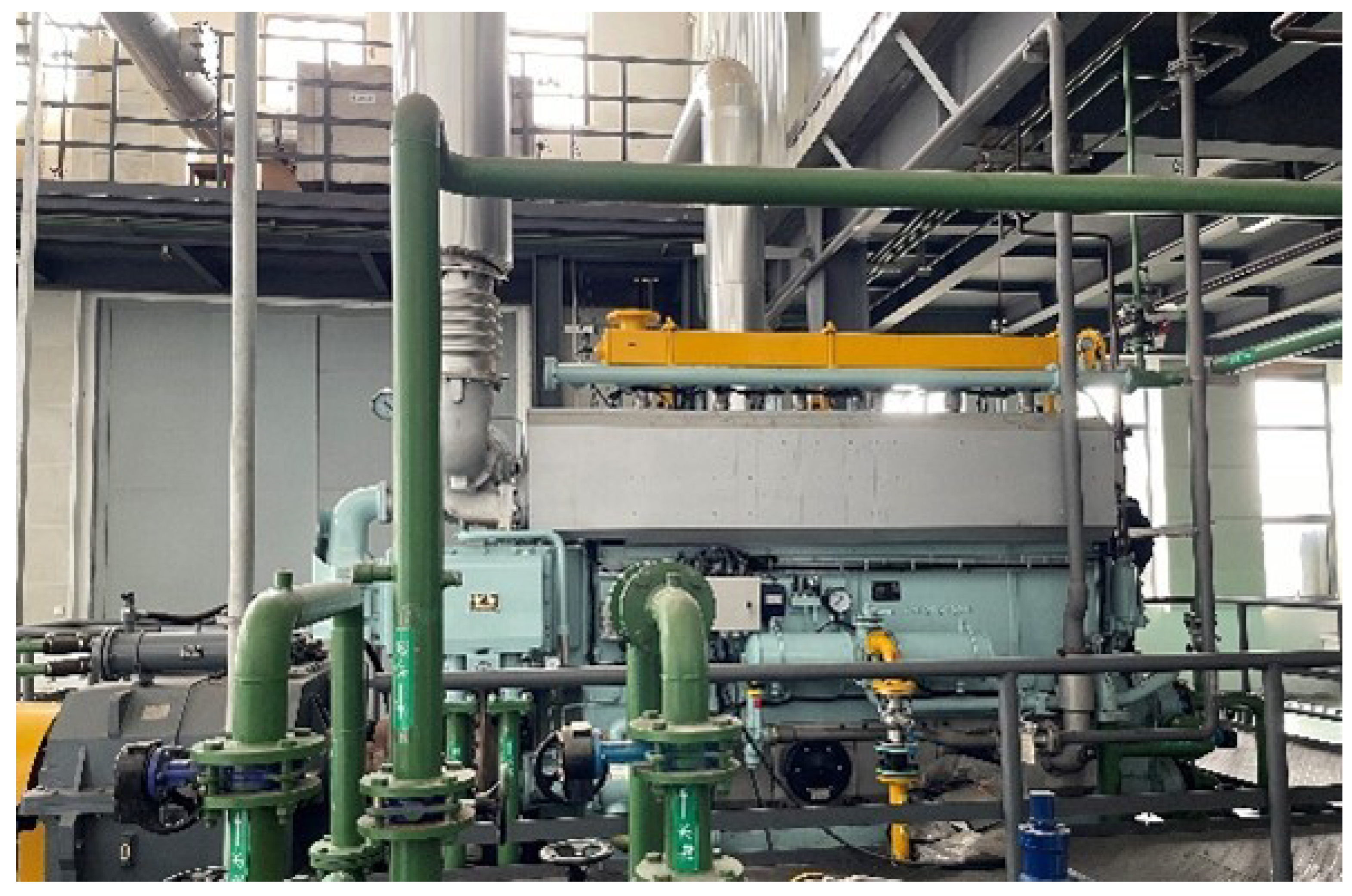
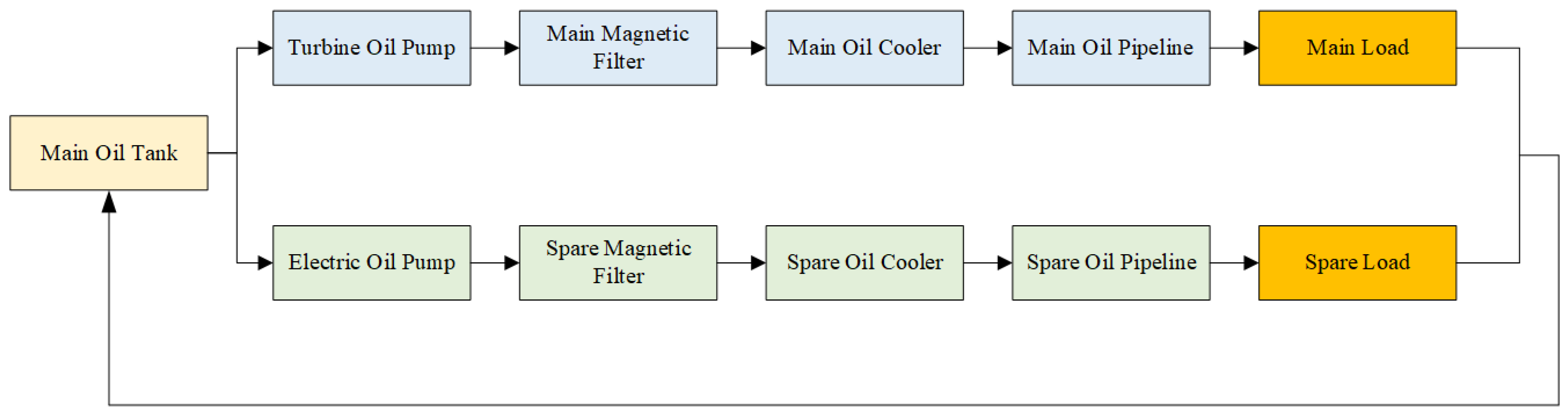
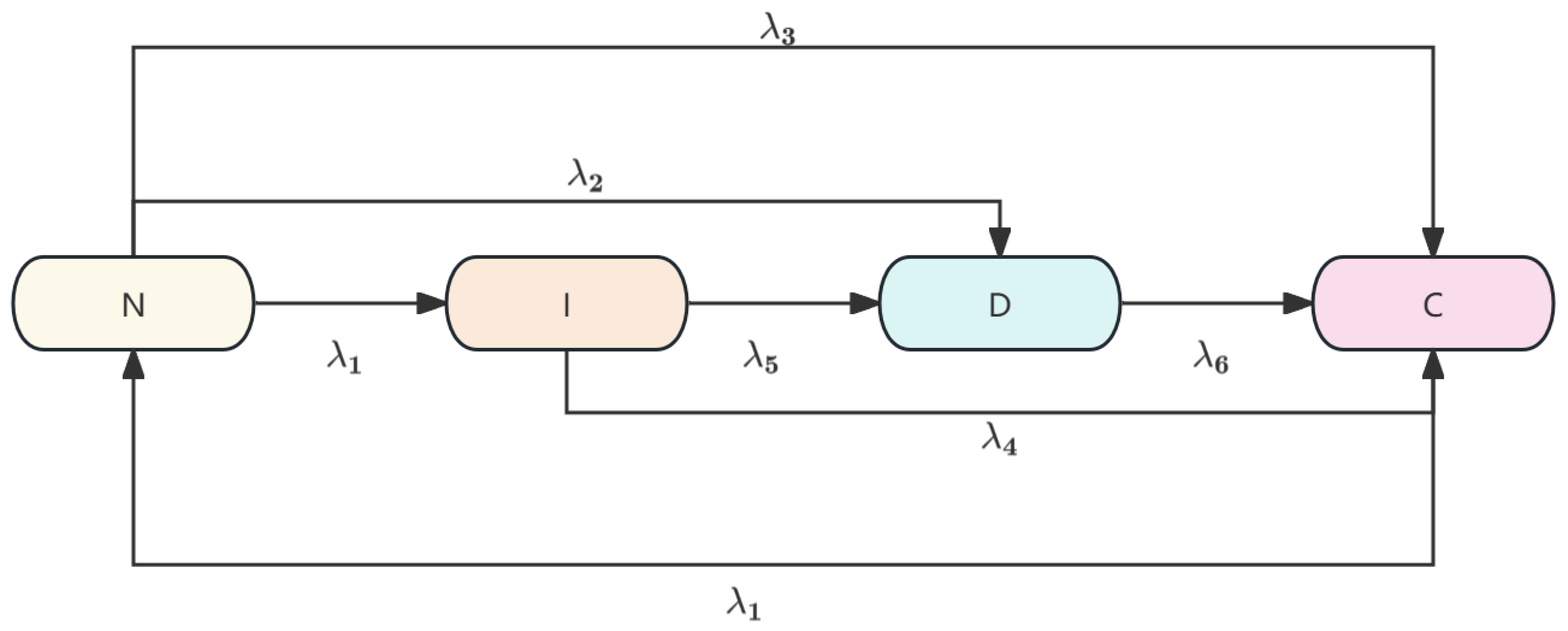
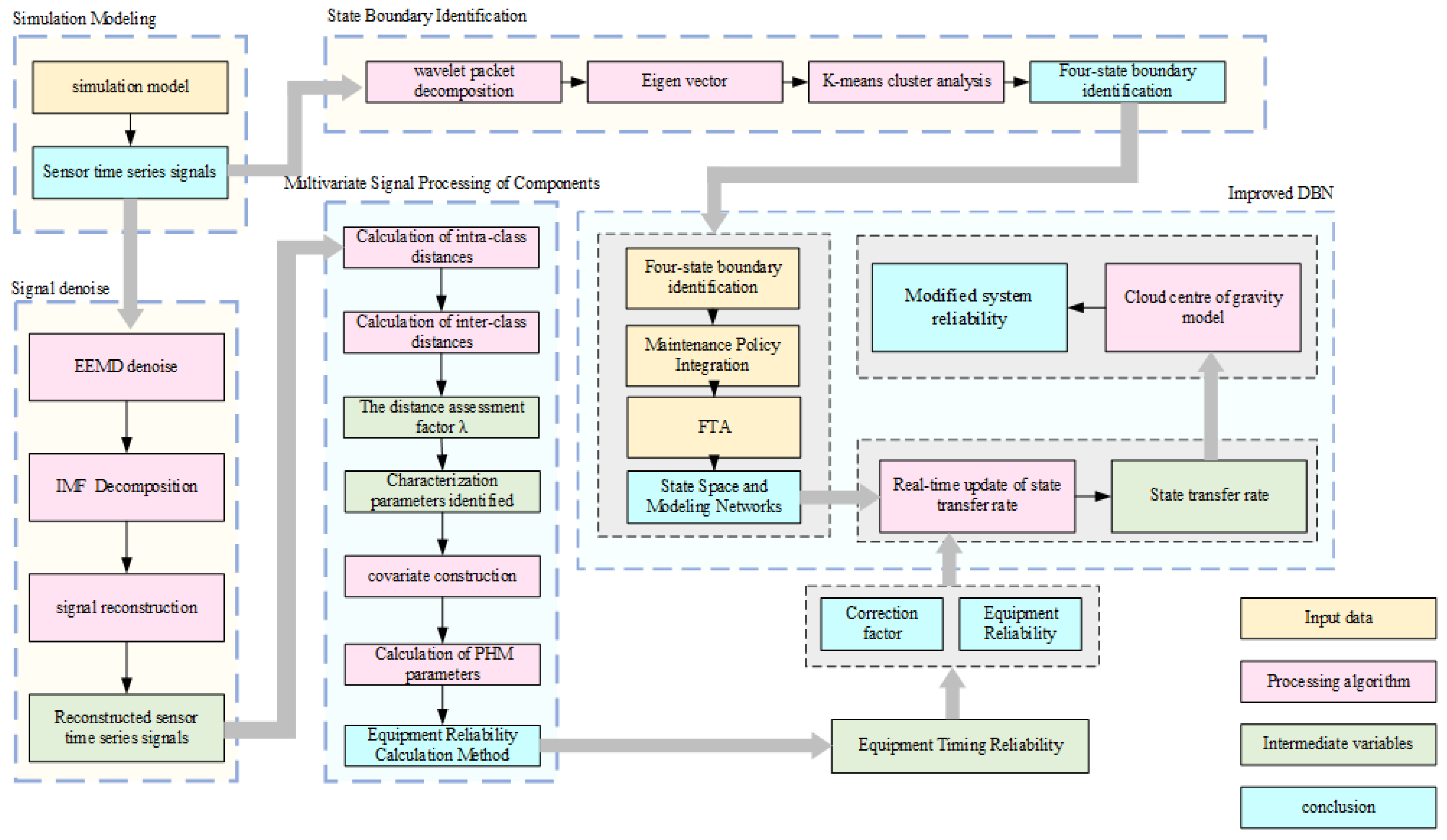
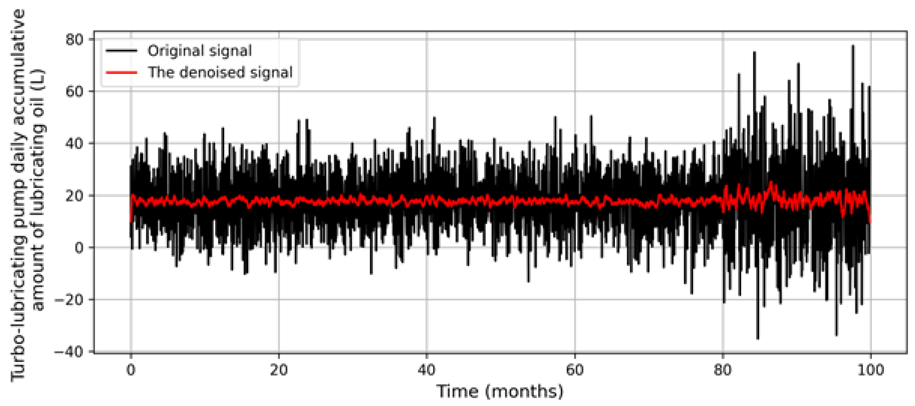
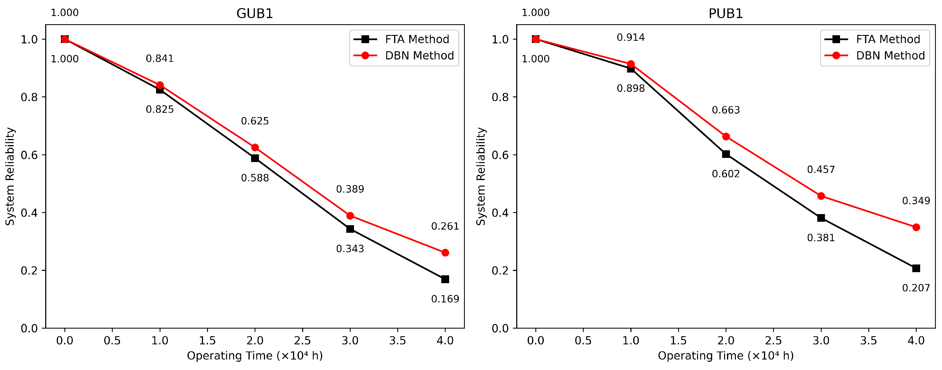
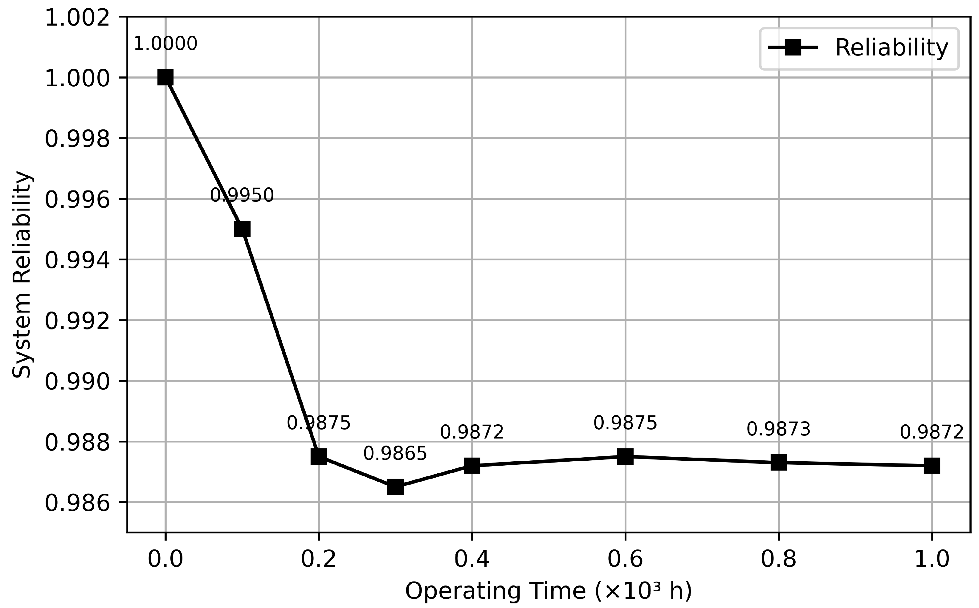