Article

Assessing Flood and Landslide Susceptibility Using XGBoost: Case Study of the Basento River in Southern Italy

1
Department of Engineering, University of Basilicata, 85100 Potenza, Italy
2
Department for Humanistic, Scientific, and Social Innovation, University of Basilicata, 75100 Matera, Italy
*
Author to whom correspondence should be addressed.
Appl. Sci. 2025, 15(10), 5290; https://doi.org/10.3390/app15105290
Submission received: 3 April 2025 / Revised: 2 May 2025 / Accepted: 3 May 2025 / Published: 9 May 2025

Abstract

:
Floods and landslides are two distinct natural phenomena influenced by different conditioning factors, though some environmental triggers may overlap. This study applied eXtreme Gradient Boosting (XGBoost) to develop susceptibility maps for both phenomena, using a unified approach based on the same geospatial predictors. The approach integrated topographical, geological, and remote sensing datasets. Flood event data were collected from institutional sources using multi-source and high-resolution remotely sensed data. The landslide inventory was compiled based on historical records and geomorphological analysis. Key conditioning factors such as elevation, slope, lithology, and land cover were analyzed to identify areas prone to floods and landslides. The methodology was applied to the Basento River basin in Southern Italy, a region frequently impacted by both hazards, to assess its vulnerability and inform risk management strategies. While flood susceptibility is primarily associated with low-lying areas near river networks, landslides are more influenced by steep slopes and geological instability. The XGBoost model achieved a classification accuracy close to 1 for flood-prone areas and 0.92 for landslide-prone areas. Results showed that flood susceptibility was primarily associated with low Elevation and Relative Elevation, and high Drainage Density, whereas landslide susceptibility was more influenced by a broader and balanced set of factors, including Elevation, Drainage Density, Relative Elevation, Distance and Lithology. The resulting susceptibility maps offered critical approaches for land use planning, emergency management, and risk mitigation. Overall, the results demonstrated the effectiveness of XGBoost in multi-hazard assessments, offering a scalable and transferable approach for similar at-risk regions worldwide.

1. Introduction

Since the impacts of natural hazard disasters are expected to intensify in the future due to the combined effects of climate change, rapid global population growth, and urbanization [1,2], all nations are paying close attention to the necessity of considering the long-term impacts of natural hazards. According to the UN General Assembly, a hazard is “a process, phenomenon or human activity that may cause loss of life, injury or other health impacts, property damage, social and economic disruption or environmental degradation”. Natural hazards can be categorized as geophysical, hydrological, climatological, meteorological, or biological. They may also be categorized as rapid onsets such as flash floods, landslides, earthquakes, and volcanic eruptions as well as slow onsets such as droughts, increasing temperatures, sea level rise, glacial retreat, etc. [3]. Among them, floods and landslides, recognized as rapid-onset disasters, produce the most fatalities because of the rapid accumulation of surface runoff often exacerbated by intense rainfall [4]. Floods are the costliest in terms of economic damage in Europe and one of the most frequent hazards worldwide [5,6]. According to records from the World Bank, approximately 3.7 million square kilometers of land worldwide are vulnerable to landslides, affecting an estimated 300 million people [2,7]. In Italy, a total of 50,593 fatalities were recorded across 2580 floods and landslide events between 1279 and 2002 based on the database of both floods and landslides [8,9].
Floods and landslides are inevitable natural hazards that pose significant threats to human settlements, environment, and economy [7]. The susceptibility map serves as a crucial initial step to predict the potential spatial extents across various scales for adequate planning and effective risk management at mitigating damage and enhancing resilience against them [2,10,11]. Various methods, including qualitative, quantitative, and semi-quantitative methods, are employed to assess the susceptibility maps for floods and landslides. In the case of landslides, common methods include inventory-based analyses, physically-based slope models, statistical methods, and knowledge-based approaches [12,13,14]. Similarly, flood susceptibility mapping uses multi-criteria decision-making (MCDM) techniques, physically based hydrological models, statistical methods, and knowledge-based approaches [10,15]. Recently, knowledge-based approaches, particularly machine learning models, have been increasingly applied in susceptibility mapping for both floods and landslides to enable a less complex implementation, testing, and validation with high-performance output compared to the traditional ones [10,12,16]. These models are considered cost-effective and capable of highly accurate output through complex mathematical formulations and precise input data to provide a high performance of models [2]. Various machine learning models such as artificial neural network (ANN), logistic regression (LR), support vector machine (SVM), decision tree (DT), and ensemble techniques such as bagging and boosting are used in susceptibility mapping of floods and landslides [14]. The predictive performance of conventional machine learning models such as ANN, LR, and SVM can be improved by advanced ensemble techniques such as bagging and boosting [14,17,18].
Advanced ensemble techniques have gained preference among researchers for susceptibility modeling of floods and landslides. Various tree-based ensemble learning models, such as Random Forest (RF), Adaptive Boosting (AdaBoost), Categorical Boosting (CatBoost), Light Gradient Boosting Machine (LightGBM), and eXtreme Gradient Boosting (XGBoost), have been widely employed due to their robust predictive capabilities [7,13,19]. Dawson et al. [20] conducted flood susceptibility mapping in England using three machine learning models: Classification and Regression Trees (CART), Random Forest (RF), and eXtreme Gradient Boosting (XGBoost). Among these, XGBoost showed the highest predictive performance, achieving a receiver operating characteristic (ROC) curve value of 0.93. Similarly, Akinci [13] evaluated the performance of various machine learning models, including artificial neural networks (ANN), Gradient Boosting Machine (GBM), RF, and support vector machine (SVM), for rainfall-induced landslide susceptibility mapping across three districts in Artvin, Türkiye. The study found that GBM exhibited the highest prediction accuracy, achieving a prediction rate of 97%. Moreover, Akinci and Ozalp [7] applied the XGBoost model for landslide susceptibility mapping in the districts of Trabzon, Rize, and Artvin, Türkiye, highlighting its superior performance from earlier studies while comparing with other machine learning models on landslides, floods, and forest fires. Similarly, Can et al. [17] conducted a comprehensive assessment of landslide susceptibility by applying the XGBoost model in the upper basin of the Ataturk Dam, Türkiye, achieving an area under the curve (AUC) value of 0.96, indicating high predictive accuracy. So far, previous studies have typically focused on a single type of hazard, using either a single machine learning model or multiple machine learning approaches.
The selection of conditioning factors is crucial to obtaining effective prediction models [12,14]. Generally, the topographic (slope aspect, slope, elevation, profile curvature, plan curvature), hydrologic (aridity, topographic wetness index (TWI), moisture index), geologic (soil type, land use), environmental (climate, watershed, drainage pattern, vegetation), and human-related factors (distance to roads, distance to cities, distance to the drainage network) have been major contributions to flood occurrence and landslide formation [12,14,15]. However, Akinci and Ozalp [7] stated that there are no specific criteria for choosing conditioning factors and specific characteristics of the study area, and the data availability plays a crucial role.
This study proposed a new unified approach to multi-hazard susceptibility mapping by employing a single machine learning model, XGBoost, based on the same geospatial predictors for both flood and landslide assessment. The analysis was conducted in the Basento River basin, southern Italy, integrating high-resolution topographic, geological, and remote sensing data. The conditioning factors were selected based on the main literature review and data availability, particularly high-resolution satellite imagery and geospatial datasets of the study area used for flood and landslide mapping. The methodology combined advanced data pre-processing techniques, correlation analysis between conditioning factors and observed events, and explainable AI methods (SHAP) to assess the contribution of each variable to the final predictions. The rest of the paper is organized as follows: Section 2 describes the study area, data sources, and the methodology adopted for flood and landslide susceptibility mapping using the XGBoost model. The geospatial conditioning factors and the inventory data are also detailed. Section 3 presents the results of the susceptibility analyses, including model performance metrics and an interpretability analysis based on SHAP values, which highlight the relative importance of each input variable. Section 4 discusses the findings in the context of previous literature, outlining the strengths, limitations, and practical implications. Conclusions are provided at the end.

2. Materials and Methods

2.1. Study Area

The Basento River, located in southern Italy, is one of the main rivers of Basilicata (Figure 1). It originates in the Lucanian Apennine at an elevation of approximately 1200 m above sea level and flows for about 149 km before emptying into the Ionian Sea. The river drains a basin of approximately 1535 km2, covering diverse geomorphological zones, including mountainous, hilly, and coastal areas [21]. The river’s upper course is characterized by steep slopes and highly erodible lithologies, contributing to frequent landslides. In the middle and lower sections, the Basento crosses wide alluvial plains where sediment transport and deposition processes dominate. The river is prone to seasonal flooding, particularly during intense rainfall events in autumn and winter. The Basento River basin in southern Italy represents a highly vulnerable area to extreme hydrogeological events, particularly floods and landslides. The combination of geological, climatic, and anthropogenic factors makes this region prone to significant natural hazards, which have historically caused severe impacts on infrastructure, human settlements, and the environment [7].
Historical records and remote sensing analyses have documented significant flood events, including those of March 2011, October 2013, and December 2013. These events caused widespread damage to infrastructure, agricultural land, and local communities, necessitating extensive emergency response efforts. The study area is characterized by low-lying floodplains, insufficient drainage capacity, and increasing land-use pressure, exacerbating flood risks. Similarly, landslides pose a persistent threat to the region, with over 1000 recorded events between 1925 and 2015, as analyzed by Dal Sasso et al. [22]. The high density of landslide occurrences, particularly in the hilly and mountainous areas of the basin, is attributed to the presence of unstable clayey and marly formations, as well as prolonged intense rainfall.

2.2. Flood Inventory Map

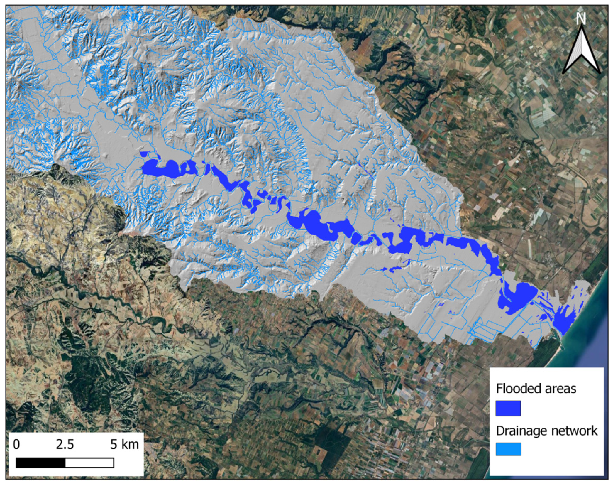
As documented by De Musso et al. [23], high-resolution remote sensing data were crucial in mapping the spatial evolution of the flood event, demonstrating how extreme precipitation combined with the region’s geomorphology have led to widespread flooding. To develop a comprehensive geodatabase of historical flood events along the Basento River, information on historically flooded areas was collected and harmonized from various institutional datasets, including those from the Basilicata Region, the Southern Apennines District Basin Authority, and the University of Basilicata. The acquisitions of the flood extent derive from data available on the Copernicus Emergency (CMS) platform and COSMO-SkyMed (CSK) images supplied by the Italian Space Agency (ASI) upon request from the DPC. The latter were obtained in Stripmap mode with a 2.5 m resolution and characterized by horizontal or vertical polarization. Additional details regarding the investigated events and satellite imagery are documented in recent scientific publications [23,24,25]. Specifically, the datasets used to support this study’s objectives include the following:
  • March 2011 flood event: For this event, RGB images of the flooded areas acquired by Cosmo-SkyMed and provided by ASI to the DPC were georeferenced. Subsequently, a semi-automated supervised classification procedure was applied to identify the pixels affected by the flooding.
  • October 2013 flood event: Flood extent maps were made available by the Copernicus EMS service, with acquisitions from the SPOT-6 satellite on October 17th, 2013, at 11:40 AM.
  • December 2013 flood event: Flood extent maps were provided for the Ionian coast of Basilicata, referring to the acquisitions from December 2nd and 3rd at 4:31 AM. Furthermore, the Copernicus EMS portal enabled the integration of this information with satellite acquisitions from December 4th and 5th at 10:55 AM and 12:55 PM, respectively. This allowed the creation of a map highlighting the evolution of the flood events in the affected area.
The validation map of historical flood events from multiple data sources is illustrated in Figure 2.

2.3. Landslide Inventory Map

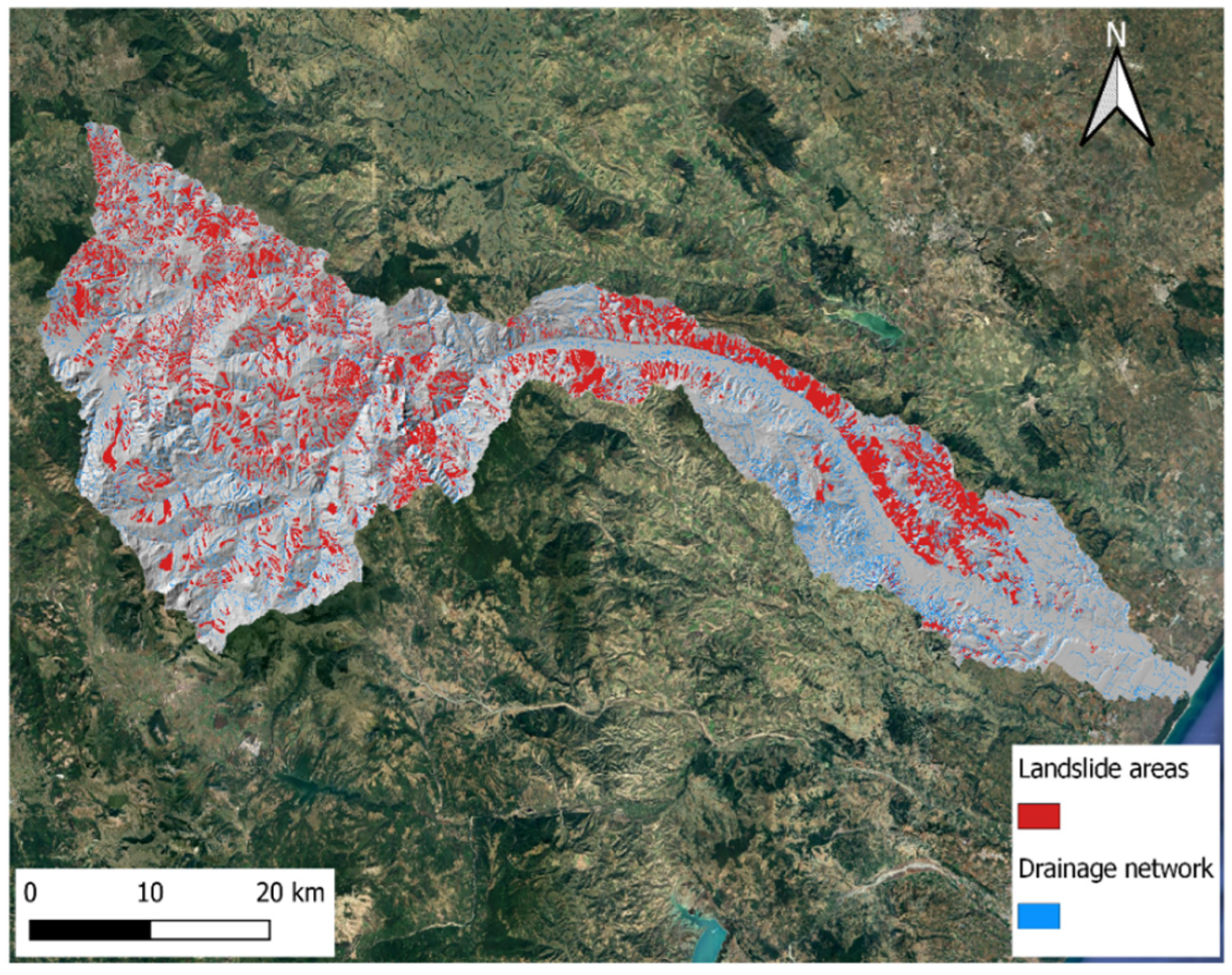
High-resolution Digital Elevation Models (DEMs with 5 m spatial resolution) were employed in the GIS platform to identify spatial distribution and highlight the main features of the Basento River basin mass movements. Landslide data were acquired and processed from official databases, including PAI (Piano Assetto Idrogeologico) and IFFI (Inventario dei Fenomeni Franosi in Italia), with an amount of 12,812 and 3736 data, respectively. To standardize the databases, some kinematics were adjusted and merged (e.g., slow and rapid flow were merged into “earthflow”, and rotational and translational slides were combined into “roto-translational”), while others were excluded—such as Deep-Seated Gravitational Slope Deformations (DSGSDs), areas requiring hydrological verifications, badland areas, slopes subject to diffuse retreat, retrogressive phenomena. Specifically, the kinematics considered for the present work are the following: earthflow, roto-translational, complex landslide, surficial landslide, rock fall, sinkhole, and lateral spread. The validation map of historical landslide events is illustrated in Figure 3.

2.4. Conditioning Factors

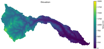
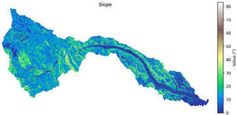
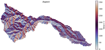
The flood and landslide susceptibility assessment in the Basento basin integrated multiple conditioning factors derived from high-resolution geospatial data and pro-cessed using Geographic Information Systems (GIS) and remote sensing techniques. These factors included Elevation, Slope, Aspect, Relative Elevation, Drainage Network, Land Use, Curve Number (CN), Lithology, Distance from the Drainage Network, and Drainage Density, each playing a crucial role in identifying landslide and flood-prone areas [12,14,15]. Slope, Aspect, Relative Elevation, Drainage Network, and Drainage Density were extracted from the Digital Terrain Model (DTM) with a pixel size of 20 × 20 m using spatial analyst tools available in the ArcGIS 10.3 software.
The elevation map was obtained from the official geospatial datasets of the Basilicata Region, specifically from airborne LiDAR surveys and photogrammetric processing. The dataset was resampled to a 20 m resolution, ensuring uniformity across the study area. Before analysis, preprocessing steps such as gap filling, interpolation of NoData values, and edge matching were performed to eliminate inconsistencies between adjacent tiles. The finalized DTM provides fundamental elevation data for calculating derivative topographic parameters.
The slope map was derived from the DTM using standard GIS-based gradient calculations; the slope was computed for each cell using a 3 × 3 m moving window and the planar method, which identifies the steepest rate of elevation change.
The aspect map was computed using the planar method, which identifies the orientation of the maximum slope gradient. Derived from the DTM through standard GIS calculations, the aspect is classified into eight cardinal directions (N, NE, E, SE, S, SW, W, NW).
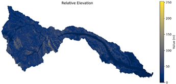
The relative elevation, representing the difference in height between a given location and the nearest drainage point, was computed to assess localized susceptibility. It was determined by subtracting the base level elevation (associated with nearby river channels) from the surface elevation of each pixel.
The distance to the drainage network was computed using GIS-based Euclidean distance analysis, assigning each pixel a value corresponding to its shortest distance from the nearest river or stream. In addition to standard Euclidean distance, a flow-path distance approach was also applied, simulating the actual hydraulic connectivity between terrain points and the drainage system.
The drainage density was computed by dividing the total stream length within a predefined grid cell by the cell’s area, using a moving window analysis in GIS. The resulting map highlights areas with high drainage density, which correspond to regions with more developed fluvial networks and higher flood risk potential.
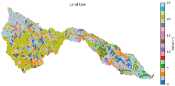
The land use map was obtained from the Regional Spatial Data Infrastructure (RSDI), which provides geospatial datasets for environmental monitoring and spatial planning. The dataset is derived from the CORINE Land Cover 2012 classification at a 1:100,000 scale, offering 44 distinct land cover classes grouped into three hierarchical levels.
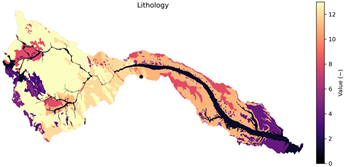
The geolithological map was implemented using both a 5 m-resolution Digital Elevation Model (DEM) derived from LiDAR data available on the geoportal of the Basilicata Regional Authority (http://rsdi.regione.basilicata.it/) (accessed on 2 May 2025) and official topographic maps by the Italian ‘Istituto Geografico Militare’ (IGM) at a 1:25,000 scale. Geological maps at a 1:50,000 scale and, where the 1:50,000-scale maps are not yet available, geological maps at a 1:100,000 scale, were used to draw the boundaries of the lithological units, together with data from edited or unpublished geological maps at different scales [26]. The Basento River basin is characterized by sedimentary units, Mesozoic to Quaternary in age. The following are the lithological units considered: (1) Present-day and recent loose and/or locally/weakly cemented cover deposits; (2) Sands; (3) Gravels and sands; (4) Clay-sandy breccias; (5) Conglomerates with weakly cemented sandstone and silty clay; (6) Sandstone with clay; (7) Clay with sandstone and conglomerate; (8) Sandstones and marly clays; (9) Clay, marls, and limestone; (10) Siliceous sedimentary rocks; (11) Limestone with chert beds and nodules; (12) Platform (i.e., shallow-water) limestone and dolostone.
The sources and characteristics of the spatial data of each conditioning factor can be found in Table 1.

2.5. Susceptibility Modeling

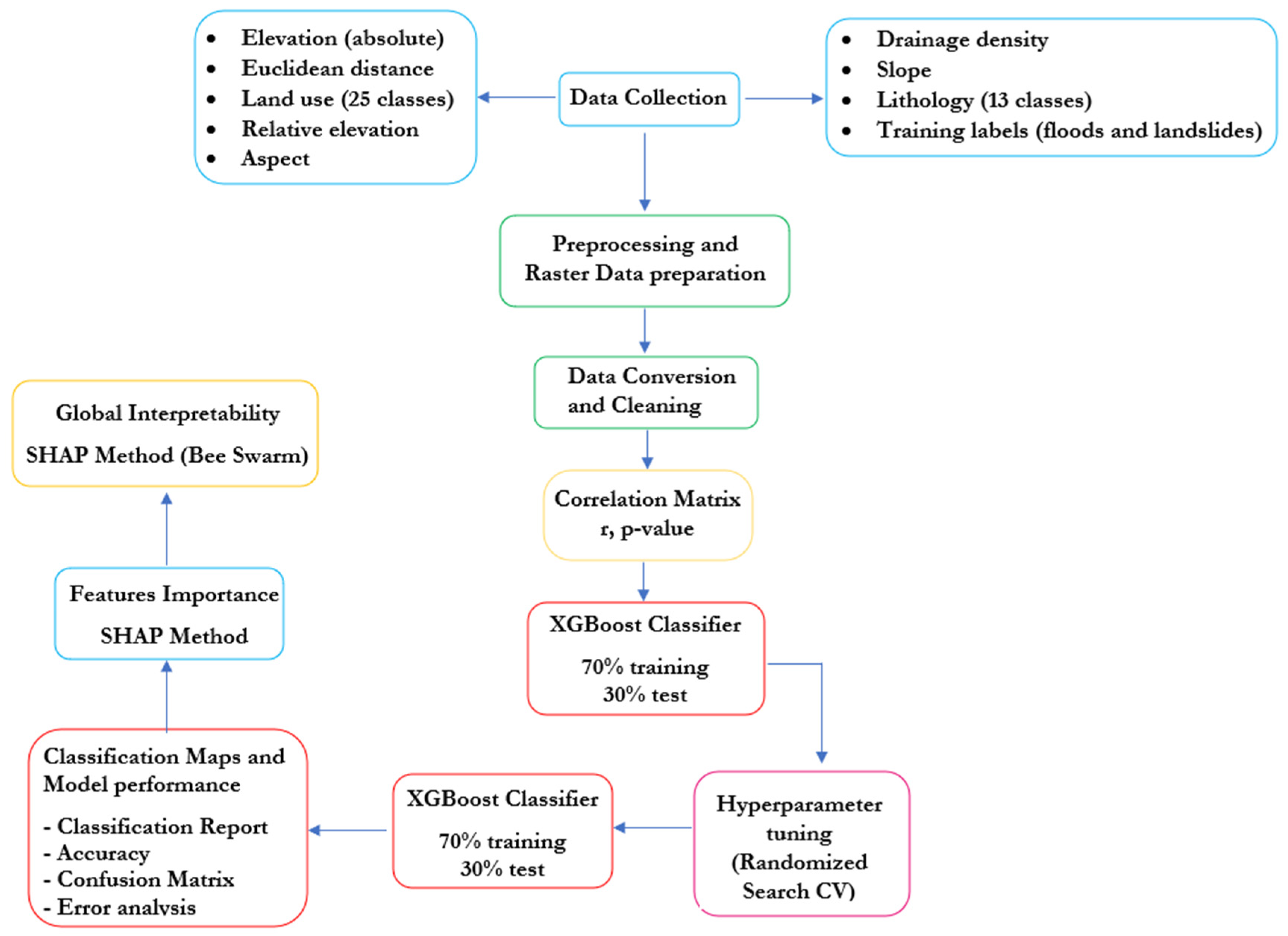
This study aimed to identify the conditioning factors that may influence the occurrence of landslide and flooding events. To achieve this, the XGBoost machine learning model was applied and the SHAP method (SHapley Additive exPlanation) was employed to assess and validate the model. The methodological workflow is illustrated in Figure 4 and is systematically outlined in the following five steps.
  • In the initial phase, pre-processing and raster data preparation (10 conditioning factors) were carried out, which allowed us to (1) align the raster cells to ensure spatial consistency among data from different sources; (2) convert raster data into 1D vectors to simplify processing; (3) reduce the raster resolution by 80% to optimize data management; (4) visualize raster data to visually identify patterns or anomalies.
  • In the data conversion and cleaning phase, the following steps were performed: (1) replace NoData values with NaN to properly handle missing data; (2) apply numeric encoding of categorical variables such as land use and lithology; (3) transform raster data from 2D matrices to 1D vectors to simplify data handling; (4) create a DataFrame containing the raster variables and target for analysis; (5) remove NaN values to ensure a complete dataset ready for analysis.
  • Subsequently, a correlation analysis was performed between the conditioning factors and the targeted variables, i.e., the flooded areas and the landslide areas [27]. The analysis was conducted by applying Pearson’s correlation coefficient, which measures the relationship between two datasets: if the value is close to 1 (−1), it indicates a strong positive (negative) correlation, meaning both datasets increase (decrease) together; if the value is close to 0, it indicates no correlation. In this study, no substantial correlation was observed between the conditioning factors for both flooded and landslide-prone areas. Consequently, none of the factors were excluded from the analysis.
  • Then, the XGBoost model was trained using 70% of the dataset, while the remaining 30% was used for testing to validate the model’s performance for both flood and landslide susceptibility mapping. The dataset, which included flooded and landslide areas, served as the target variable, while the 10 conditioning factors were used as predictors for susceptibility modeling.
The XGBoost model, used as a supervised classification model [28], was initially introduced by Chen and Guestrin [29]. This algorithm is an optimized version of the Gradient Boosting Machine (GBM) and employs a gradient boosting framework combined with decision tree-based ensemble learning [30,31]. XGBoost is particularly effective in reducing prediction and classification errors due to its capacity to adapt to complex and non-linear datasets. The algorithm combines weak decision trees to create a complex and accurate model. It functions by sequentially adding decision trees, with each new tree enhancing the performance of the previous one by following the gradient direction of the loss function. The objective function, which assesses the model’s error during training, consists of two components: a loss function that measures the discrepancy between actual and predicted values, and a regularization term that penalizes model complexity to reduce the risk of overfitting. The XGBoost model employs optimization techniques during training, such as parallel computation to expedite tree construction, optimized splitting strategies to choose the best splits at the nodes, and advanced handling of missing values without requiring explicit imputations. The model’s performance is assessed using accuracy as a key metric. It was further improved through hyperparameter tuning to boost its performance using the Randomized Search CV method. This approach randomly selects combinations of values from predefined ranges and evaluates them through cross-validation. In the context of an XGBoost classification model, this strategy enables efficient exploration of the extensive hyperparameter space, including parameters like tree depth, learning rate, and the number of trees. By avoiding the need to evaluate all possible combinations, this method enhances performance while significantly reducing computational costs. Consequently, the tuning process is expedited, allowing for the swift identification of the optimal configuration for accurately classifying the areas in question. Following the workflow shown in Figure 4, after hyperparameter optimization, the classification model is reapplied, and its performance is reevaluated. Additionally, a classification report and a confusion matrix are used to assess classification results by identifying true positives, true negatives, false positives, and false negatives, thus providing a thorough analysis of the model’s predictive capability. Furthermore, an error analysis is performed to gain a deeper understanding of the model’s performance. Finally, a feature importance analysis is conducted to identify the most influential factors.
5.
Lastly, the weight of each variable to the model’s predictions is assessed by determining the extent to which each independent variable influences the target variable. This is achieved using the SHAP method [32,33,34], a popular approach in Explainable Artificial Intelligence (XAI) [35], commonly used in game theory. The SHAP method calculates the Shapley value for each predictor in the model, and the relation is written as follows.
ϕ i = S N \ i S ! N S 1 ! N ! · [ v   S   i v ( S ) ]
where ϕi is the Shapley value for each predictor i; N is the set of all predictors; S is a subset of predictors that does not include i; v(S) is the value function (model prediction) for subset S. The main objective of XAI methods is to make the functioning of artificial intelligence models transparent, avoiding so-called “black box” processes. Through XAI methods, the importance of each observed variable can be evaluated to determine its influence on the predicted values. Based on this hypothesis, it is possible to estimate the reliability of the model. Additionally, Bee Swarm plots are applied to obtain a clear idea of the most significant variables and their corresponding values (global interpretability).

3. Results

The results of the preliminary analysis and the assessment of the XGBoost model’s performance, corresponding to steps (3), (4), and (5) in Section 2.5, are presented in the following sections.

3.1. Preliminary Analysis and Application of the XGBoost Classifier

The preliminary phase of this study (step 3, Section 2.5) evaluated the relationship between the conditioning factors and the target variables considered (flooded areas and landslide areas) in the Basento River basin. The Pearson correlation coefficients and the corresponding correlation matrix were computed for both flood and landslide phenomena, with a significance threshold (p-value) set at 0.01, to determine the statistical significance of the observed correlations, as illustrated in Figure 5.
In this preliminary analysis, the correlations obtained were generally weak for both flood-prone areas (Figure 5a) and landslide-prone areas (Figure 5b). This suggested the lack of a strong correlation either among the selected conditioning factors or between these factors and the two target variables considered. Consequently, none of the examined conditioning factors were excluded from the modeling process. Subsequently, an XGBoost machine learning model was applied for the classification of areas at risk of floods and landslides. This involved dividing the dataset into two parts: one for training the model (70%) and the other for testing it (30%).

3.2. Model Performance Analysis

The model’s performance was evaluated by analyzing the classification report for flood-prone areas as presented in Table 2. The classification report provided a comprehensive summary of the performance of the XGBoost classification model. In Table 2, it can be observed that the XGBoost model achieved exact classification for class 0 (representing non-flooded areas), with both precision and recall close to 1. However, a slight decrease in performance was noted for class 1 (flooded areas), where precision and recall were 84% and 96%, respectively. This performance discrepancy was attributed to class imbalance, as the support for class 0 is significantly higher (i.e., 1,025,456) compared to class 1 (i.e., 11,150). It is important to emphasize that class imbalance should not be considered a drawback of the modeling process, as it naturally reflects the distribution of flood-prone and non-flood-prone areas within the basin. The number of flood-prone areas is inherently smaller than that of those regions where flooding does not occur. The initial labeling map used for classification represented a snapshot of the study area at a specific point in time. Further analysis of the classification report indicated that the model demonstrated strong overall performance, as evidenced by high accuracy, macro average, and weighted average values. With a total of 1,036,606 instances considered, these metrics suggested the robustness and reliability of the XGBoost model in classifying flood-prone areas.
As shown in Table 2, it is evident that the model shows extremely high performance in classifying flood events—with an accuracy of 0.997—raising concerns about the possible presence of overfitting. To assess the model’s generalization capability and verify this hypothesis, a systematic performance analysis was carried out across different validation levels (Table 3).
The results obtained from the 10-fold cross-validation show a remarkable stability of the metrics across the different folds: precision ranges from 0.801 to 0.819, recall from 0.964 to 0.968, F1-score from 0.878 to 0.887, and accuracy remains 0.997. This consistency across folds indicated that the model did not excessively fit the training data specific to each fold, suggesting a robust and generalizable learning process. These findings were further confirmed by the independent test set (30% of the data, not used during training), where the model achieved high values in line with those observed in the cross-validation. In the presence of overfitting, one would expect significantly higher metrics on the training/CV phases compared to the test set; however, in the current study, no performance drop was observed. On the contrary, the metrics on the test set were even slightly higher than the average from cross-validation (e.g., mean F1-score of 0.882), further supporting the hypothesis of a well-generalized model. An additional contribution to mitigating overfitting came from the use of the SMOTE (Synthetic Minority Over-sampling Technique) during the training phase. This technique helped balance the classes by generating synthetic examples of the minority class, improving the model’s fairness and generalization capability. In summary, the absence of significant divergences between the performances achieved on training (with SMOTE), cross-validation, and test sets, combined with the balanced distribution of errors and the consistency of the metrics, provided strong evidence that the model does not suffer from overfitting.
In Table 4, it can be observed that the model accurately identified class 0 (non-landslide-prone areas), achieving strong classification performance. However, a slight decrease in performance was noted for class 1 (landslide-prone areas), as indicated by lower recall and F1-score values. This decrease suggested that the model was not fully capturing all landslide-prone areas, leading to the omission of some high-risk zones. Specifically, only 79% of landslide-prone areas were correctly recognized. Similarly, class imbalance was observed (with a support of 949,477 for class 0 and 196,004 for class 1), although it was less pronounced than what could be observed for flooded areas. The model achieved an accuracy of 92%, confirming that, overall, it performed well across all instances (1,145,481).
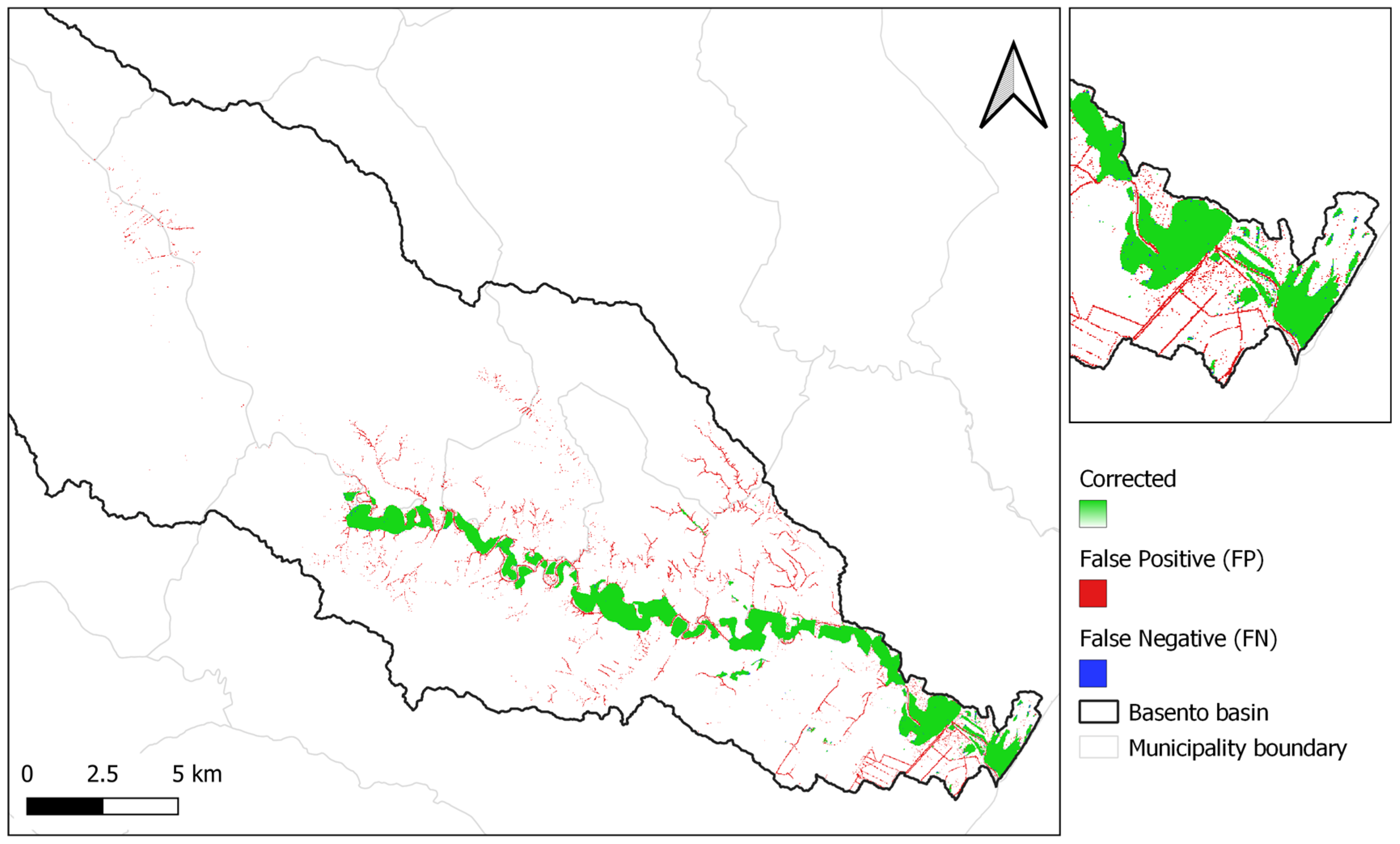
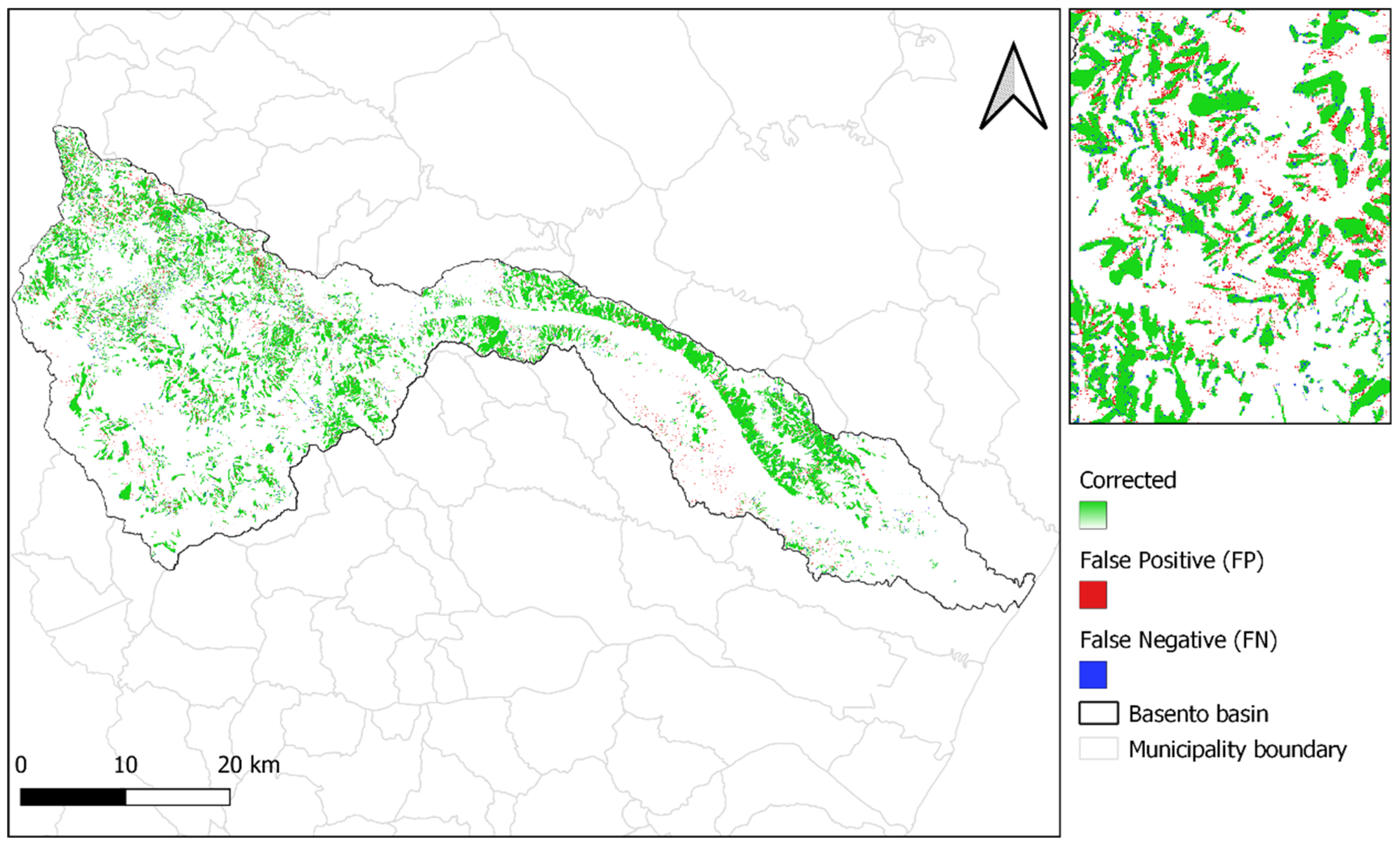
It is important to note that both models used the same conditioning factors, which may require differentiation depending on whether flooding or landslide phenomena are being analyzed. The lack of distinction between these factors could contribute to the observed decrease in XGBoost’s performance for landslide prediction compared to its performance in identifying flood-prone areas. Additionally, the analysis of the model’s performance was concluded with the error maps illustrated in Figure 6 and Figure 7.
As shown in Figure 6, which was related to flood-prone areas, the model correctly classified many areas of the basin. Only a small number of areas were classified as either false-positive (0.06%) or false-negative (1.24%) flood-prone areas. This observation further reinforced the earlier discussion, confirming that the model exhibited excellent performance in accurately classifying flood-prone areas. Figure 7 shows the results obtained for landslide areas and, similarly, the model correctly classified the landslide areas. Only a few cases were false-positive (2.07%) and false-negative (6.48%) landslide areas, both in the upstream and downstream zones of the basin, following the recall and accuracy results obtained.
Additionally, it is possible to assess the percentage contribution of each conditioning factor to the classification (Figure 8), which is crucial for understanding which parameters should be considered relevant in the classification of flood-prone and landslide-prone areas. The feature importance was reported based on the SHAP method.
As illustrated in Figure 8, which refers to flood-prone areas, the SHAP analysis provided a clear overview of the relative importance and behavior of the conditioning factors. In Figure 8a, elevation emerged as the most influential variable, contributing to 50% of the model’s predictions. Following this, relative elevation accounted for 17%, and drainage density contributed to 9%, leading to a cumulative importance of 76%. This threshold aligned with the general assumption that the most relevant features were those whose combined contribution reached at least 70–80%. These findings highlighted that flood susceptibility in the study area was predominantly influenced by terrain morphology and drainage structure.
A closer look at the relative contributions (Figure 8a) revealed that, although relative elevation ranks second, its importance was not markedly higher than that of drainage density. This confirmed the dominance of elevation as the single most impactful factor in flood susceptibility mapping, with other variables contributing with moderate but significant influence. The complementary Bee Swarm plot in Figure 8b further supported these observations, illustrating not only the relative importance of the variables but also how their values influenced the model’s predictions. Specifically, flooding was more likely to occur in areas with low elevation and relative elevation, while high drainage density values were positively associated with flood-prone areas. In contrast, variables such as slope showed limited relevance, as indicated by both their low SHAP scores and minimal percentage contributions.
Regarding landslide susceptibility, Figure 9 shows the SHAP-based analysis for landslide-prone areas. In Figure 9a, the contributions of the conditioning factors appeared more balanced: elevation (23%) and drainage density (16%) were among the most influential, yet no single factor dominated the model. This suggested a more complex interplay of variables in triggering landslide events compared to floods. Following the same cumulative contribution logic, the most relevant variables identified included elevation, drainage density, relative elevation, distance, and lithology. The Bee Swarm plot in Figure 9b reinforced these insights by showing that landslide occurrence was generally associated with low elevation, relative elevation, and lithology values, whereas higher drainage density and distance values tended to increase susceptibility. Moreover, the SHAP score distributions were relatively uniform across the top predictors, confirming that no single conditioning factor dominated in the case of landslides, thus highlighting the need for a multifactorial approach when modeling complex geo-morphological hazards such as landslides.

4. Discussion

This study investigated the use of Extreme Gradient Boosting (XGBoost) to model flood and landslide susceptibility within the Basento River basin in southern Italy. The findings showed the model’s strong predictive capability, particularly in identifying flood-prone areas, through the integration of topographic, geological, and remote sensing data. Flood susceptibility mapping achieved higher accuracy than landslide susceptibility, likely due to the relatively simpler and more consistent conditioning factors involved—such as low elevation and proximity to drainage networks—compared to the more variable factors influencing landslides, such as slope stability and lithological heterogeneity. Additionally, the completeness of landslide inventories was often lower, which may further affect the model’s performance.
The analysis showed that flood-prone areas were primarily associated with low elevation, relative elevation, and high drainage density. In contrast, landslide-prone areas were influenced by a broader and less uniform set of variables, including elevation, drainage density, relative elevation, distance, and lithology. These results aligned with previous studies in the field [15,17,20], yet this study offered a novel contribution by employing a single, unified machine learning model for both hazard phenomena. The use of multi-source satellite data (e.g., Copernicus EMS, COSMO-SkyMed) further improved the robustness of the predictions. Practically, the generated susceptibility maps served as valuable tools for spatial planning, infrastructure development, and risk mitigation. They allowed decision makers to prioritize interventions in the most vulnerable areas. The key innovative aspects of this work include the following:
  • A unified multi-hazard modeling approach, using the same framework to assess both flood and landslide susceptibility, overcoming the traditional separation between these two analyses.
  • Integration of multi-source data, including high-resolution satellite imagery (Copernicus EMS, COSMO-SkyMed) and geospatial datasets, enhancing the reliability of predictions.
  • The use of SHAP analysis to interpret the model’s decisions and understand the impact of different predisposing factors, ensuring transparency and interpretability.
  • A scalable and transferable model, which can be adapted to other geographical areas with similar hazards, supporting land-use planning and risk management.
Nonetheless, several limitations emerged. The lower performance for landslides reflected their complex and heterogeneous nature. Since the current model was based solely on spatial variables, integrating temporal indicators—such as rainfall intensity, soil moisture variation, and vegetation dynamics—could substantially improve accuracy. A further limitation was the potential incompleteness and spatial bias of the landslide inventory. Unlike floods, which can be more directly mapped from satellite imagery, landslide delineation and categorization often require expert interpretation. Increasing the spatial and temporal resolution of landslide data would enhance the model’s performance. Moreover, while a unified set of predictors simplifies implementation, it may overlook hazard-specific characteristics.
The misclassification errors observed can be attributed, in part, to factors such as the different spatial resolution of the data and the geomorphological complexity of the studied areas. The input maps used in the model, derived from official sources, while widely accepted and reliable for risk modeling, may not have a high enough spatial resolution to capture finer, localized features of the landscape.
In particular, areas with subtle topographical variations or complex morphological configurations (such as partially urbanized floodplains or slopes with local fractures) can introduce uncertainties in the predictor values, which in turn may negatively affect the model’s classification accuracy. Moreover, areas with dense vegetation or recent anthropogenic changes not well represented in the available datasets may also lead to errors in classification.
These methodological developments are closely linked to the practical goals of this study. The proposed framework is designed to support spatial planning, emergency response, and territorial risk management. In this context, future work will aim to integrate the resulting susceptibility maps into early warning systems and urban planning protocols, making the model a useful tool for operational decision making. In addition, comparative studies involving other multi-hazard-prone regions in Italy and abroad are planned to test the scalability and generalizability of the approach. Finally, building on the current findings, future applications will explore how key variables, such as drainage density and land use, respond to specific hydro-geological mitigation strategies.

5. Conclusions

This study applied XGBoost, an advanced machine learning technique, to assess flood and landslide susceptibility in the Basento River basin, southern Italy. By integrating high-resolution geospatial data, multi-source remote sensing datasets, and explainable AI methods (SHAP analysis), the research developed a robust and interpretable multi-hazard prediction framework. The main findings are summarized as follows:
  • XGBoost showed excellent predictive performance, achieving a classification accuracy of 100% for flood susceptibility and 92% for landslide susceptibility.
  • SHAP analysis enabled interpretability, revealing that low elevation, relative elevation, and high drainage density were the most influential predictors for flood events, whereas elevation, drainage density, relative elevation, distance, and lithology were the key contributors to landslide susceptibility.
  • The unified modeling framework allowed for the simultaneous evaluation of multiple hazard types using a single set of predictors, providing a scalable and transferable methodology for other regions facing similar risks.
  • The integration of remote sensing products (e.g., Copernicus EMS, COSMO-SkyMed) and GIS-based conditioning factors improved the spatial resolution and reliability of susceptibility maps, supporting more informed decision making in land-use planning, infrastructure design, and emergency response.
Overall, this study confirmed that XGBoost, when combined with explainable AI techniques, was a powerful and practical tool for multi-hazard risk assessment. The proposed framework could be readily adapted to other regions to support data-driven disaster mitigation strategies, enhance climate adaptation planning, and contribute to sustainable territorial management. To further enhance the robustness and applicability of the proposed framework, future studies could incorporate landslide data with higher spatial and temporal resolution, as well as extend the analysis to include additional natural hazards such as wildfires. Integrating time-variant variables such as precipitation intensity, NDVI (Normalized Difference Vegetation Index), evapotranspiration (ETP), and soil moisture content would also improve the model’s responsiveness, enabling more dynamic and accurate susceptibility assessments.

Author Contributions

Conceptualization, M.F., M.S., S.F.D.S. and V.T.; methodology, S.F.D.S. and V.T.; software, M.R. and H.H.A.; validation, S.F.D.S. and V.T.; formal analysis, S.F.D.S. and V.T.; investigation, M.S., L.C., G.D., M.R., H.H.A., S.F.D.S. and V.T.; data curation, M.S., L.C., G.D., M.R., H.H.A., S.F.D.S. and V.T.; writing—original draft preparation, M.R., H.H.A., S.F.D.S. and V.T.; writing—review and editing, M.S., L.C., G.D., M.R., H.H.A., S.F.D.S. and V.T.; visualization, M.S., L.C., G.D., M.R., H.H.A., S.F.D.S. and V.T.; supervision, M.F., M.S., S.F.D.S. and V.T. All authors have read and agreed to the published version of the manuscript.

Funding

This research received no external funding.

Institutional Review Board Statement

Not applicable.

Informed Consent Statement

Not applicable.

Data Availability Statement

Data are contained within the article.

Conflicts of Interest

The authors declare no conflicts of interest.

References

  1. Cremen, G.; Galasso, C.; McCloskey, J. Modelling and quantifying tomorrow’s risks from natural hazards. Sci. Total Environ. 2022, 817, 152552. [Google Scholar] [CrossRef] [PubMed]
  2. Sujatha, E.R.; Sudharsan, J.S. Landslide Susceptibility Mapping Methods—A Review. In Landslide: Susceptibility, Risk Assessment and Sustainability Advances in Natural and Technological Hazards Research; Springer Nature: Berlin, Germany, 2024; pp. 87–102. [Google Scholar]
  3. Tosun, J.; Howlett, M. Managing slow onset events related to climate change: The role of public bureaucracy. Curr. Opin. Environ. Sustain. 2021, 50, 43–53. [Google Scholar] [CrossRef]
  4. Modrick, T.M.; Georgakakos, K.P. The character and causes of flash flood occurrence changes in mountainous small basins of Southern California under projected climatic change. J. Hydrol. Reg. 2015, 3, 312–336. [Google Scholar] [CrossRef]
  5. Johnstone, W.M.; Lence, B.J. Assessing the value of mitigation strategies in reducing the impacts of rapid-onset, catastrophic floods. J. Flood Risk Manag. 2009, 2, 209–221. [Google Scholar] [CrossRef]
  6. Albano, R.; Limongi, C.; Dal Sasso, S.F.; Mancusi, L.; Adamowski, J. Flood scenario spatio-temporal mapping via hydrological and hydrodynamic modelling and a remote sensing dataset: A case study of the Basento river (Southern Italy). Int. J. Disaster Risk Reduct. 2024, 111, 104758. [Google Scholar] [CrossRef]
  7. Akinci, H.; Ozalp, A.Y. Investigating the Effects of Different Data Classification Methods on Landslide Susceptibility Mapping. Adv. Space Res. 2025, 75, 3427–3450. [Google Scholar] [CrossRef]
  8. Guzzetti, F. Landslide fatalities and the evaluation of landslide risk in Italy. Eng. Geol. 2000, 58, 89–107. [Google Scholar] [CrossRef]
  9. Guzzetti, F.; Stark, C.P.; Salvati, P. Evaluation of flood and landslide risk to the population of Italy. Environ. Manag. 2005, 36, 15–36. [Google Scholar] [CrossRef]
  10. Mudashiru, R.B.; Sabtu, N.; Abustan, I. Quantitative and semi-quantitative methods in flood hazard/susceptibility mapping: A review. Arab. J. Geosci. 2021, 14, 941. [Google Scholar] [CrossRef]
  11. Albano, R.; Adamowski, J. Use of digital elevation models for flood susceptibility assessment via a hydrogeomorphic approach: A case study of the Basento River in Italy. Nat. Hazards 2025. [Google Scholar] [CrossRef]
  12. Azarafza, M.; Akgun, H.; Atkinson, P.M.; Derakhshani, R. Deep learning-based landslide susceptibility mapping. Sci. Rep. 2021, 11, 24112. [Google Scholar] [CrossRef] [PubMed]
  13. Akinci, H. Assessment of rainfall-induced landslide susceptibility in Artvin, Turkey using machine learning techniques. J. Afr. Earth. Sci. 2022, 191, 104535. [Google Scholar] [CrossRef]
  14. Liu, S.; Wang, L.; Zhang, W.; He, Y.; Pijush, S. A comprehensive review of machine learning-based methods in landslide susceptibility mapping. Geol. J. 2023, 58, 2283–2301. [Google Scholar] [CrossRef]
  15. Kaya, C.M.; Derin, L. Parameters and methods used in flood susceptibility mapping: A review. J. Water Clim. Change 2023, 14, 1935–1960. [Google Scholar] [CrossRef]
  16. Albertini, C.; Gioia, A.; Iacobellis, V.; Petropoulos, G.P.; Manfreda, S. Assessing multi-source random forest classification and robustness of predictor variables in flooded areas mapping. Remote Sens. Appl. Soc. Environ. 2024, 35, 101239. [Google Scholar] [CrossRef]
  17. Can, R.; Kocaman, S.; Gokceoglu, C. A Comprehensive Assessment of XGBoost Algorithm for Landslide Susceptibility Mapping in the Upper Basin of Ataturk Dam, Turkey. Appl. Sci. 2021, 11, 4993. [Google Scholar] [CrossRef]
  18. Hitouri, S.; Mohajane, M.; Lahsaini, M.; Ali, S.A.; Setargie, T.A.; Tripathi, G.; D’Antonio, P.; Singh, S.K.; Varasano, A. Flood Susceptibility Mapping Using SAR Data and Machine Learning Algorithms in a Small Watershed in Northwestern Morocco. Remote Sens. 2024, 16, 858. [Google Scholar] [CrossRef]
  19. Ma, M.; Zhao, G.; He, B.; Li, Q.; Dong, H.; Wang, S.; Wang, Z. XGBoost-Based Method for Flash Flood Risk Assessment. J. Hydrol. 2021, 598, 126382. [Google Scholar] [CrossRef]
  20. Dawson, G.; Butt, J.; Jones, A.; Fraccaro, P. Flood susceptibility mapping at the country scale using machine learning approaches. Appl. AI Lett. 2023, 4, e88. [Google Scholar] [CrossRef]
  21. Schiattarella, M.; Giano, S.I.; Gioia, D. Long-term geomorphological evolution of the axial zone of the Campania-Lucania Apennine, Southern Italy: A review. Geol. Carpathica 2017, 68, 57–67. [Google Scholar] [CrossRef]
  22. Dal Sasso, S.F.; Manfreda, S.; Capparelli, G.; Versace, P.; Samela, C.; Spilotro, G.; Fiorentino, M. Hydrological and geological hazards in Basilicata. L’Acqua 2017, 3, 77–85. [Google Scholar]
  23. De Musso, N.M.; Capolongo, D.; Refice, A.; Lovergine, F.P.; D’Addabbo, A.; Pennetta, L. Spatial evolution of the December 2013 Metaponto plain (Basilicata, Italy) flood event using multi-source and high-resolution remotely sensed data. J. Maps 2018, 14, 219–229. [Google Scholar] [CrossRef]
  24. Lacava, T.; Ciancia, E.; Faruolo, M.; Pergola, N.; Satriano, V.; Tramutoli, V. Analyzing the December 2013 Metaponto Plain (Southern Italy) Flood Event by Integrating Optical Sensors Satellite Data. Hydrology 2018, 5, 43. [Google Scholar] [CrossRef]
  25. Scarpino, S.; Albano, R.; Cantisani, A.; Mancusi, L.; Sole, A.; Milillo, G. Multitemporal SAR data and 2D hydrodynamic model flood scenario dynamics assessment. ISPRS Int. J. Geo-Inf. 2018, 7, 105. [Google Scholar] [CrossRef]
  26. Schiattarella, M.; Giannandrea, P.; Corrado, G.; Gioia, D. Landscape planning-addressed regional-scale mapping of geolithological units: The example of Basilicata, southern Italy. J. Maps 2024, 20, 2303335. [Google Scholar] [CrossRef]
  27. Gogtay, N.J.; Thatte, U.M. Principles of Correlation Analysis. J. Assoc. Physicians India 2017, 65, 78–81. [Google Scholar]
  28. Shetty, S.H.; Shetty, S.; Singh, C.; Rao, A. Supervised Machine Learning: Algorithms and Applications. In Fundamentals and Methods of Machine and Deep Learning: Algorithms, Tools and Applications; Singh, P., Ed.; John Wiley & Sons: Hoboken, NJ, USA, 2022; pp. 1–16. [Google Scholar] [CrossRef]
  29. Chen, T.; Guestrin, C. XGBoost: A Scalable Tree Boosting System. In Proceedings of the 22nd ACM SIGKDD International Conference on Knowledge Discovery and Data Mining, San Francisco, CA, USA, 13–17 August 2016. [Google Scholar]
  30. Bhati, B.S.; Chugh, G.; Al-Turjman, F.; Bhati, N. An Improved Ensemble-Based Intrusion Detection Technique Using XGBoost. Trans. Emerg. Tel. Tech. 2020, 32, e4076. [Google Scholar] [CrossRef]
  31. Le, T.-T.-H.; Oktian, Y.E.; Kim, H. XGBoost for Imbalanced Multiclass Classification-Based Industrial Internet of Things Intrusion Detection Systems. Sustainability 2022, 14, 8707. [Google Scholar] [CrossRef]
  32. Zhang, K.; Xu, P.; Zhang, J. Explainable AI in Deep Reinforcement Learning Models: A SHAP Method Applied in Power System Emergency Control. In Proceedings of the IEEE 4th Conference on Energy Internet and Energy System Integration (EI2), Wuhan, China, 30 October–1 November 2020. [Google Scholar] [CrossRef]
  33. Mangalathu, S.; Hwang, S.H.; Jeon, J.-S. Failure Mode and Effects Analysis of RC Members Based on Machine-Learning-Based SHapley Additive exPlanations (SHAP). Approach. Eng. Struct. 2020, 219, 110927. [Google Scholar] [CrossRef]
  34. Nohara, Y.; Matsumoto, K.; Soejima, H.; Nakashima, N. Explanation of Machine Learning Models Using Shapley Additive Explanation and Application for Real Data in Hospital. Comput. Methods Programs Biomed. 2022, 214, 106584. [Google Scholar] [CrossRef]
  35. Barredo Arrieta, A.; Díaz-Rodríguez, N.; Del Ser, J.; Bennetot, A.; Tabik, S.; Barbado, A.; Garcia, S.; Gil-Lopez, S.; Molina, D.; Benjamins, R.; et al. Explainable Artificial Intelligence: A Systematic Review. Inf. Fusion 2020, 58, 82–115. [Google Scholar] [CrossRef]
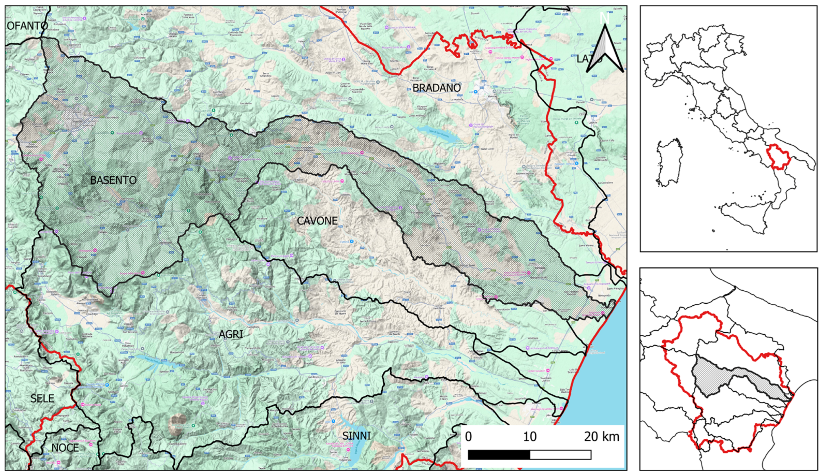
Figure 1. Geographic location of the Basento River basin.
Applsci 15 05290 g001
Figure 2. Validation map of historical flood events from multiple data sources.
Applsci 15 05290 g002
Figure 3. Validation map of historical landslide events.
Applsci 15 05290 g003
Figure 4. Flow chart of the methodology.
Applsci 15 05290 g004
Figure 5. Correlation matrix: (a) flooded areas; (b) landslide areas.
Applsci 15 05290 g005
Figure 6. Flood classification results obtained from the implementation of the optimal XGBoost model. The inset in the upper right corner provides a zoomed-in view of the Pisticci and Bernalda municipalities.
Applsci 15 05290 g006
Figure 7. Landslide classification results obtained from the implementation of the optimal XGBoost model. The inset in the upper right corner provides a zoomed-in view of the Potenza municipality.
Applsci 15 05290 g007
Figure 8. SHAP analysis for flood-prone areas: (a) feature importance based on SHAP values; (b) Bee Swarm plot showing the distribution and impact of each conditioning factor.
Applsci 15 05290 g008
Figure 9. SHAP analysis for landslide-prone areas: (a) feature importance based on SHAP values; (b) Bee Swarm plot showing the distribution and impact of each conditioning factor.
Applsci 15 05290 g009
Table 1. Sources and characteristics of the spatial data used in this study.
DataSource/ScaleMap
Elevationhttps://rsdi.regione.basilicata.it/ (accessed on 2 May 2025)
(5 m spatial resolution)
Applsci 15 05290 i001
SlopeDerivedApplsci 15 05290 i002
AspectDerivedApplsci 15 05290 i003
Relative elevationDerivedApplsci 15 05290 i004
Distance to networkDerivedApplsci 15 05290 i005
Drainage
density
DerivedApplsci 15 05290 i006
Land Usehttps://rsdi.regione.basilicata.it/ (accessed on 2 May 2025)
(1:5000)
Applsci 15 05290 i007
Lithology(1:50,000)Applsci 15 05290 i008
Table 2. Classification report for flooded area.
Classification Report
PrecisionRecallF1 ScoreSupport
00.9990.9980.9991,025,456
10.8370.9580.89311,150
accuracy 0.9971,036,606
macro avg0.9180.9780.9461,036,606
weighted avg0.9980.9980.9981,036,606
Table 3. Cross-validation in 10-fold for flooded area (class 1).
Cross Validation
No. of FoldsPrecisionRecallF1 ScoreSupport
10.8010.9680.8820.997
20.8150.9660.8840.997
30.8170.9680.8860.997
40.8030.9680.8780.997
50.8080.9680.8810.997
60.8190.9670.8870.997
70.8120.9640.8820.997
80.8030.9680.8780.997
90.8070.9670.8800.997
100.8080.9650.8790.997
μ0.8090.9670.8820.997
Test sample0.8370.9580.8930.997
Table 4. Classification report for landslide areas.
Classification Report
PrecisionRecallF1 ScoreSupport
00.960.940.95949,477
10.730.790.76196,004
accuracy 0.921,145,481
macro avg0.850.870.861,145,481
weighted avg0.920.920.921,145,481
Disclaimer/Publisher’s Note: The statements, opinions and data contained in all publications are solely those of the individual author(s) and contributor(s) and not of MDPI and/or the editor(s). MDPI and/or the editor(s) disclaim responsibility for any injury to people or property resulting from any ideas, methods, instructions or products referred to in the content.