River Surface Space–Time Image Velocimetry Based on Dual-Channel Residual Network

Abstract

Space–Time Image Velocimetry (STIV) estimates the one-dimensional time-averaged velocity by analyzing the main orientation of texture (MOT) in space–time images (STIs). However, environmental interference often blurs weak tracer textures in STIs, limiting the accuracy of traditional MOT detection algorithms based on shallow features like images’ gray gradient. To solve this problem, we propose a deep learning-based MOT detection model using a dual-channel ResNet (DCResNet). The model integrates gray and edge channels through ResNet18, performs weighted fusion on the features extracted from two channels, and finally outputs the MOT. An adaptive threshold Sobel operator in the edge channel improves the model’s ability to extract edge features in STI. Based on a typical mountainous river (located at the Panzhihua hydrological station in Panzhihua City, Sichuan Province), an STI dataset is constructed. DCResNet achieves the optimal MOT detection at a 7:3 gray–edge fusion ratio, with MAEs of 0.41° (normal scenarios) and 1.2° (complex noise scenarios), respectively, outperforming the single-channel models. In flow velocity comparison experiments, DCResNet demonstrates an excellent detection performance and robustness. Compared to current meter results, the MRE of DCResNet is 4.08%, which is better than the FFT method.

1. Introduction

The accurate and timely monitoring of hydrological parameters, particularly flow velocity and discharge, is critical for effective flood disaster prevention and mitigation [1]. During flood events, conventional contact-based measurement methods face significant challenges. High flow velocities and elevated sediment concentrations often damage instruments and endanger personnel [2]. Moreover, point measurement techniques struggle to capture the complex turbulence characteristics of natural rivers efficiently, limiting their practicality during critical flood periods. To overcome these limitations, non-contact measurement techniques have gained increasing attention in recent years [3,4,5,6]. These methods employ cameras installed along riverbanks to record water surface videos, enabling a safe and efficient flow velocity estimation by analyzing the motion vectors of natural tracers in sequential images and converting them to real-world coordinates without direct river contact. The currently well-developed technologies primarily include Large-Scale Particle Image Velocimetry (LSPIV) [7], Large-Scale Particle Tracing Velocimetry (LSPTV) [8], Optical Tracking Velocimetry (OTV) [9], and Space–Time Image Velocimetry (STIV) [10]. STIV directly estimates the one-dimensional time-averaged flow velocity by detecting the main orientation of texture (MOT) of the space–time image (STI), and it was initially proposed by Fujita et al. [10]. Owing to its high spatial resolution and real-time processing capabilities, STIV is particularly suitable for bank-based online flow measurement systems captured at small tilt angles [11]. Currently, it has been developed into software, including KU-STIV [12], Hydroview [13], AIFlow [14], and Hydro-STIV [15], which are widely used for online flow monitoring in small and medium-sized rivers.

The key to STIV is the accurate detection of MOT. Traditional MOT detection methods primarily include the Gradient Tensor (GT) [11], Two-Dimensional Autocorrelation Function (QESTA) [16], and Fast Fourier Transform (FFT) [17]. Due to the complexity and variability of natural environments, factors such as changing lighting conditions, water surface reflections, obstacles, rain, and vortexes can significantly affect the textures in STIs. When the STI is heavily impacted by noise and the flow signal formed by tracers is weak, the detection results of the above traditional methods often have gross errors. To address these issues, the following noise reduction methods have been proposed: (1) Partition weighted average method [11]. First, the STI is divided into several windows to detect the MOT separately. To quantify the texture clarity in each window, the coherency is introduced. The average MOT is calculated by coherency weighting to reduce the impact of unclear windows. (2) Standardization (STD) filtering method [16]. Calculating standard deviations for each vertical array can equalize the unevenly distributed image intensity in STIs. (3) Edge detection method [17]. Operators like Canny and Sobel are used to extract edge information that reflects the texture orientation of the image. This method suppresses the low-frequency noise and enhances the texture features. (4) Frequency domain filtering method [18,19]. By applying a fan-type filter to the magnitude spectrum image (MSI), interference noise can be removed, while the signal related to velocity is retained. However, parameters such as radius, direction, and bandwidth are sensitive in different cases, which potentially causes random errors [20]. In recent years, the rapid advancement in deep learning has led to the development of numerous high-performance neural network models. Capable of extracting highly abstract data representations, these models excel at learning intricate mapping relationships and generating precise predictions [21,22,23]. Therefore, new MOT detection methods based on deep learning have been widely proposed to solve the problem of traditional methods with many parameters and a poor robustness. Watanabe et al. [24] employ a convolutional neural network to perform multi-scale optimal selection on MSIs, while Hu et al. [25] utilize MobileNetV2 to construct a classification model. Similarly, Huang et al. [26] apply a residual network to classify STI angles directly. However, since these classification models output discrete integer values (with a resolution of 1 or 0.5 degrees), significant quantization errors arise in flow velocity calculations. Li et al. [27] introduced a ResNet50-based regression model, enabling continuous MOT output, which has been successfully implemented in a real river. However, the method exhibits limitations in feature extraction accuracy, particularly for MOT detection in complex environments. Under such conditions, the effective texture features in STIs often become obscured by noise interference, leading to a reduced detection performance. Therefore, it is necessary to design a model with stronger feature extraction capabilities to further improve the accuracy of MOT detection.

Based on the characteristic that image edge features can explicitly represent textures’ orientation, this study proposes a dual-channel residual network (DCResNet) model for MOT detection. The model employs a dual-channel architecture that processes both the original STI and edge-detected STI. Unlike existing classification methods [24,25,26], DCResNet adopts a regression-based approach to achieve continuous MOT outputs, better reflecting the natural continuity of river flow velocities. Since regression models require the learning of continuous predictions from discrete data, they demand higher-quality datasets and more robust feature extraction capabilities. Compared to the basic regression method in [27], DCResNet innovatively combines raw STI texture features with edge-enhanced representations. The adaptive threshold Sobel operator enhances edge delineation in STIs by effectively capturing boundaries that directly characterize the texture orientation. This structural emphasis enables the model to learn discriminative motion patterns, improving MOT detection’s robustness. Features extracted from both channels are weighted and fused before regression, with optimal fusion coefficients determined through systematic training on an STI dataset constructed at the Panzhihua hydrological station. The experimental results demonstrate that DCResNet outperforms single-channel models using only raw or edge-processed STIs, validating the effectiveness of the joint learning strategy. Additionally, the model exhibits strong generalization to the unknown river. Comparative evaluations against current meter measurements confirm that DCResNet achieves a higher accuracy than the FFT method.

2. Materials and Methods

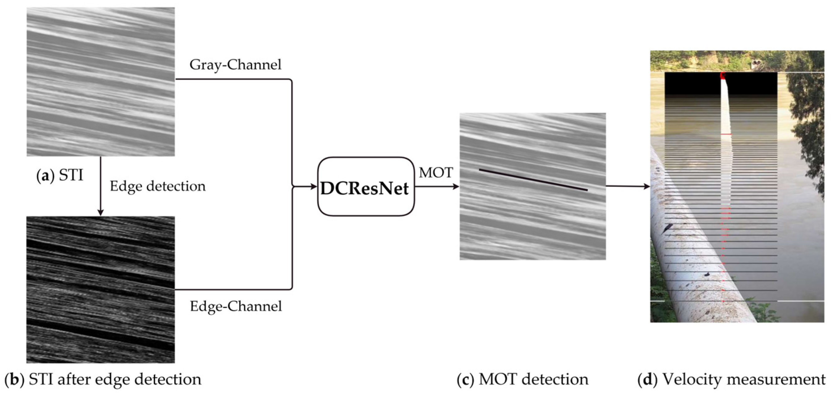
2.1. Basic Principle of STIV

STIV mainly includes three steps: synthesizing STIs, detecting the MOT, and calculating the velocity vector in the world coordinate system [10]. As shown in Figure 1, the steps of synthesizing STIs include, first, collecting $m$ consecutive frame images and then setting a set of single-pixel wide and $l$ pixels long testing lines along the flow direction in the image. Finally, the $l*m$-size STI is synthesized, with $x-t$ as the rectangular coordinate system for each testing line. The synthetic STI has significant texture features, which are manifested as bright and dark bands with a specific orientation. The angle $\delta$ between the main orientation of the texture and the vertical axis is defined as the MOT, which reflects the time-averaged water surface velocity.

In the world coordinate system, surface flow tracers move a distance $D$ along the search line within the time $T$, while in the image coordinate system, they move $d$ pixels within $\tau$ frames. Therefore, the corresponding surface velocity $V$ can be expressed as

$$V={\displaystyle \frac{D}{T}}={\displaystyle \frac{d\cdot \Delta s}{\tau \cdot \Delta t}}=\tan \delta \cdot {\displaystyle \frac{\Delta s}{\Delta t}}=v\cdot \Delta s$$

(1)

where $v$ is the optical flow motion vector, $\Delta s$ is the spatial resolution of the testing line, and $\Delta t$ is the time interval of the image sequence.

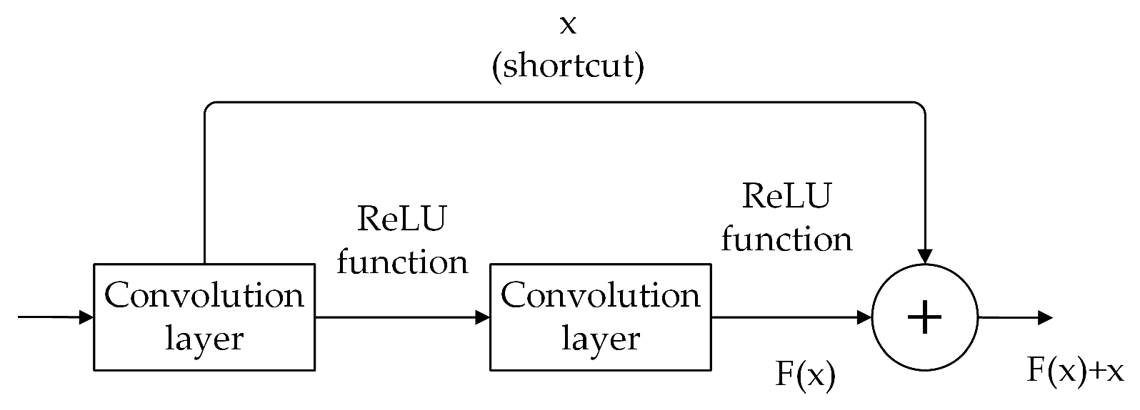
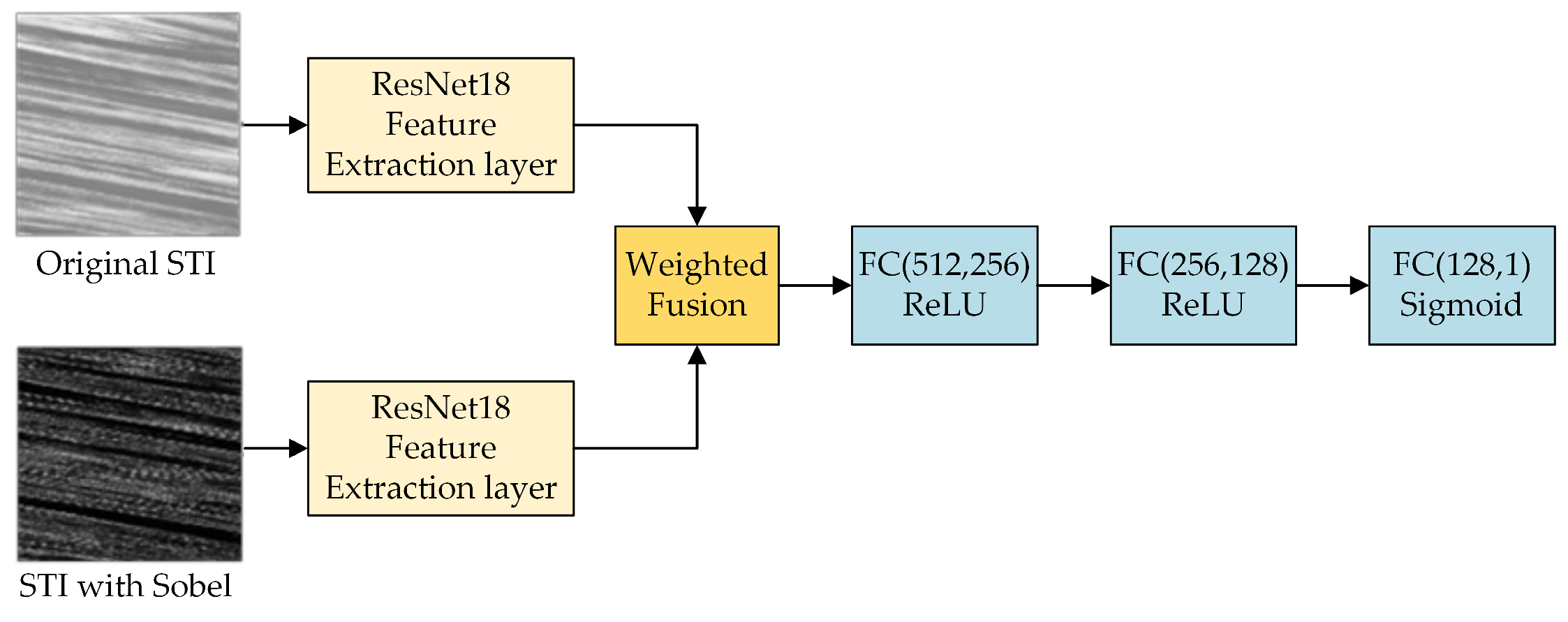
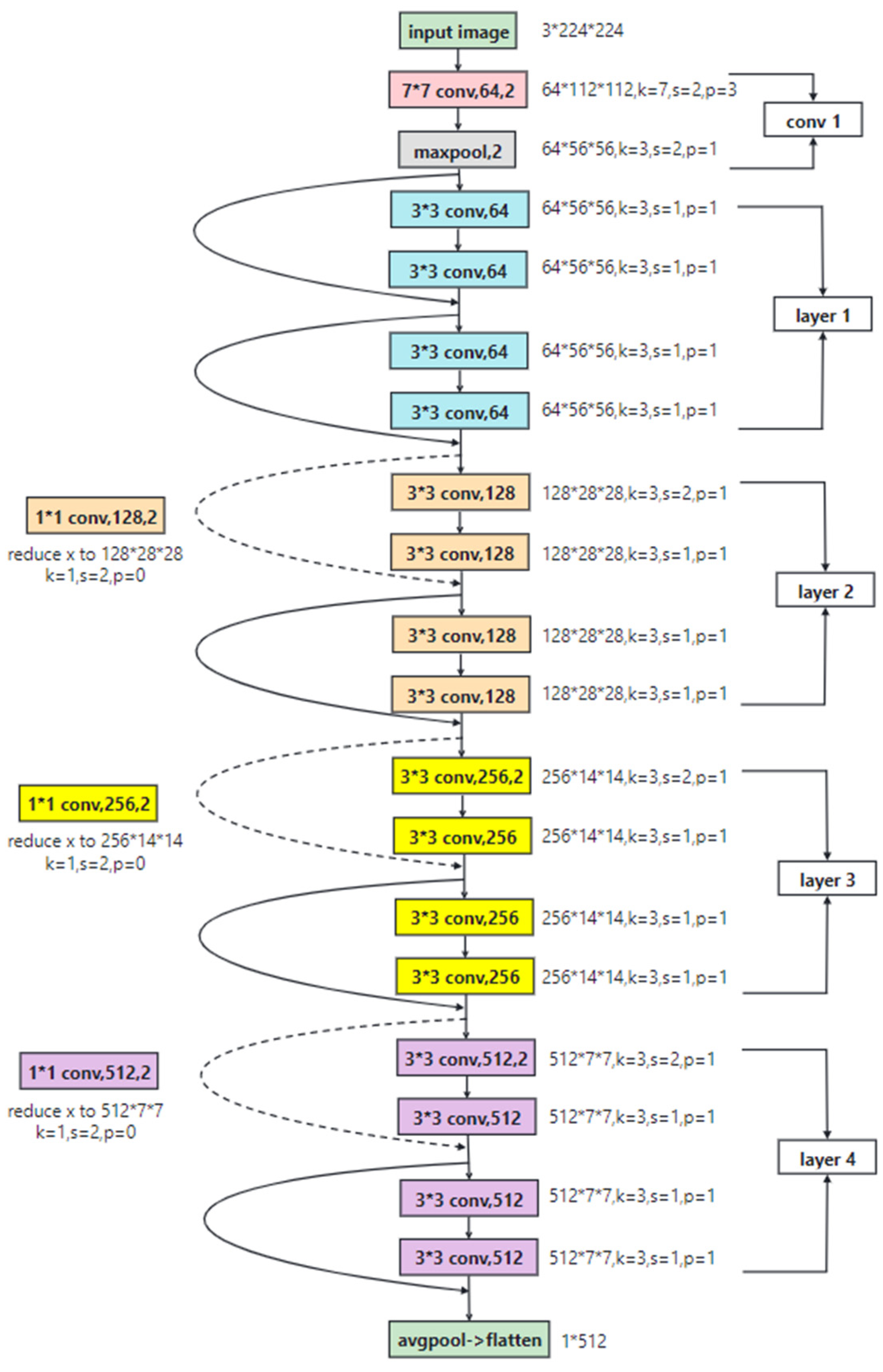
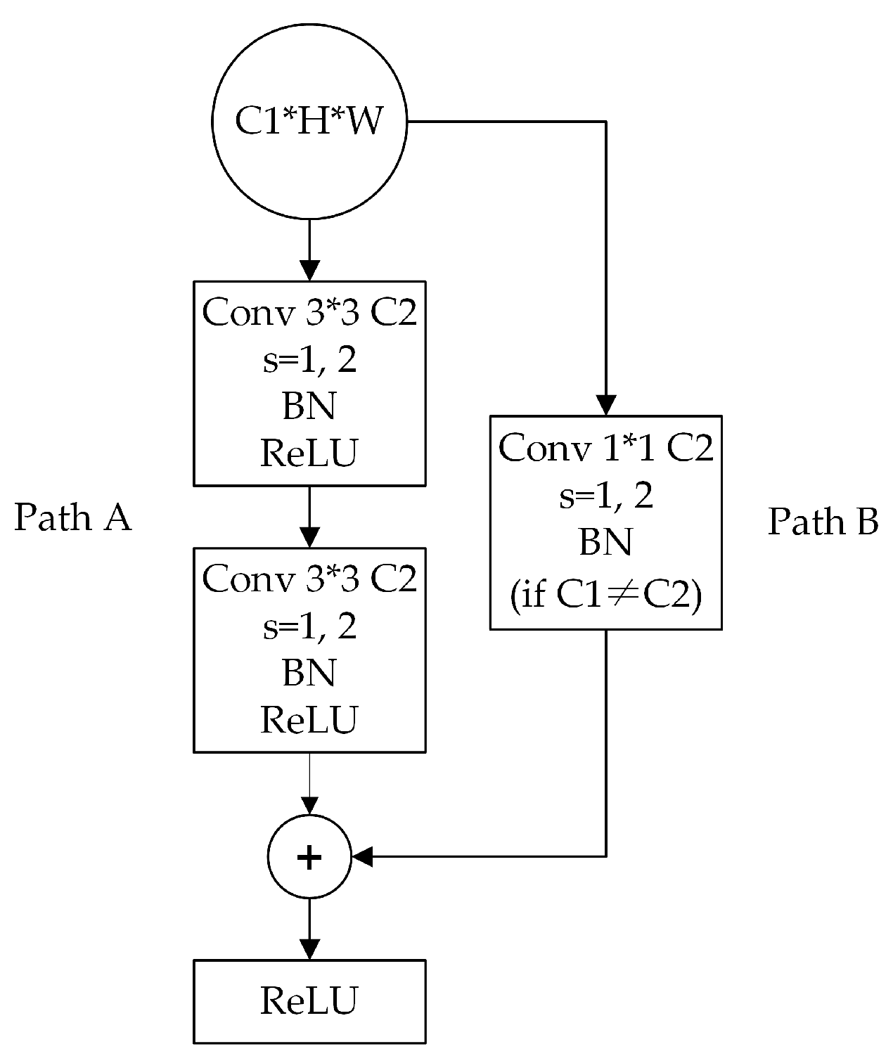
2.2. Dual-Channel Residual Network Model

The process of MOT detection is considered an image regression prediction problem:

$$\delta =F(I)$$

(2)

where $I$ is the STI to be detected, and $F$ is the regression prediction function. The residual network is used to construct the regression model, while the prediction function is constructed by its powerful image feature extraction and regression ability. Without preprocessing the STI, the MOT is directly regressed from the STI. The process of our method is shown in Figure 2. Put the STIs into the trained model to detect the MOT and calculate the velocity vector.

The idea of ResNet is to assume that there is an optimal number of network layers in a deep network, and then the network contains some redundant network layers, defined as redundant layers. Setting these redundant layers as identity layers can complete the identity mapping of the input and output, and the identity layers are learned adaptively in the process of network training [28]. Thus, the number of layers of neural networks can reach dozens, hundreds, or even thousands of layers. Figure 3 is the concrete structure of the residual block with a jump connection called the shortcut connection. The output $H(x)$ of the residual block includes the residual mapping $F(x)$ and the superposition of the input $x$. Assuming that the function mapping to be fitted is $H(x)$, then another residual mapping $F(x)$ can be defined, and $F(x)$ is equal to $H(x)-x$. It is easier to optimize the residual mapping than to optimize the original function mapping [29]. In the extreme case where the identity mapping $H(x)=x$ is optimal, the residual network only needs to learn the residual mapping to 0 ($F(x)=0$), which means it does not need to use the superimposed nonlinear network to fit the identity mapping. So ResNet can solve the problem of gradient disappearance and network degradation when building deep networks [30].

STIV mainly relies on the texture features with significant directionality formed by the tracer movement. Since edge information can well reflect the texture orientation, an edge channel is added to the gray channel to form a dual-channel residual network (DCResNet) structure. As shown in Figure 4, it mainly includes two channels and a regression layer composed of three fully connected layers. A single-channel network whose input is the original STI is denoted as Gray-Channel, while the Edge-Channel is input by the STI after Sobel detection. The weighted fusion of the above two channels is denoted as Dual-Channel.

Both channels use the feature extraction layer of ResNet18; that is, the original ResNet18 classification model removes 17 convolutional layers other than the fully connected layer. The network structure parameters are shown in Figure 5. $\mathrm{k}$ is the size of the convolution kernel, $\mathrm{s}$ is the sliding step size of the spatial domain, and $\mathrm{p}$ is the spatial domain filling. The structure of the 17-layer network can be regarded as composed of a conv1 layer and layer1-layer4 layers. The conv1 layer is a convolution layer with a convolution kernel size of $7*7$, the step size is 2, and the spatial domain filling is 3.

Layer1–layer4 are composed of two Basic Block structures. As shown in Figure 6, each Basic Block structure mainly includes two convolution layers with a convolution kernel size of $3*3$. In addition to the Basic Block in layer1, layer2–layer4 perform the down-sampling operation in the first Basic Block to ensure that the number of channels in the feature map skip connection is consistent with the number of channels in the output feature map in the Basic Block. The last convolutional layer outputs a $512*7*7$ feature map, which is processed through avgpool and flatten operations to convert it into a vector suitable for regression tasks. The avgpool operation employs a $7*7$ pooling window matching the feature map dimensions, computing the average value for each channel and compressing each $7*7$ feature map into a single scalar value, resulting in a $512*1*1$ tensor. The flatten operation then transforms this tensor into a one-dimensional vector of length 512, enabling subsequent fully connected layer operations and regression output. Since the two channels have the same network structure, the feature vectors output by the two channels at the 17th layer are also the same size, both $1*512$. The weighted fusion of features extracted by the two channel networks are as follows:

$$F=\alpha \cdot F_{original}+(1-\alpha )\cdot F_{Sobel}$$

(3)

where $\alpha$ is the normalized weighted fusion coefficient, $F_{original}$ and $F_{sobel}$ are the feature vectors extracted from the grayscale and edge channels, respectively, and $F$ is the feature vector after the weighted fusion. The value of $\alpha$ will be determined by experiments.

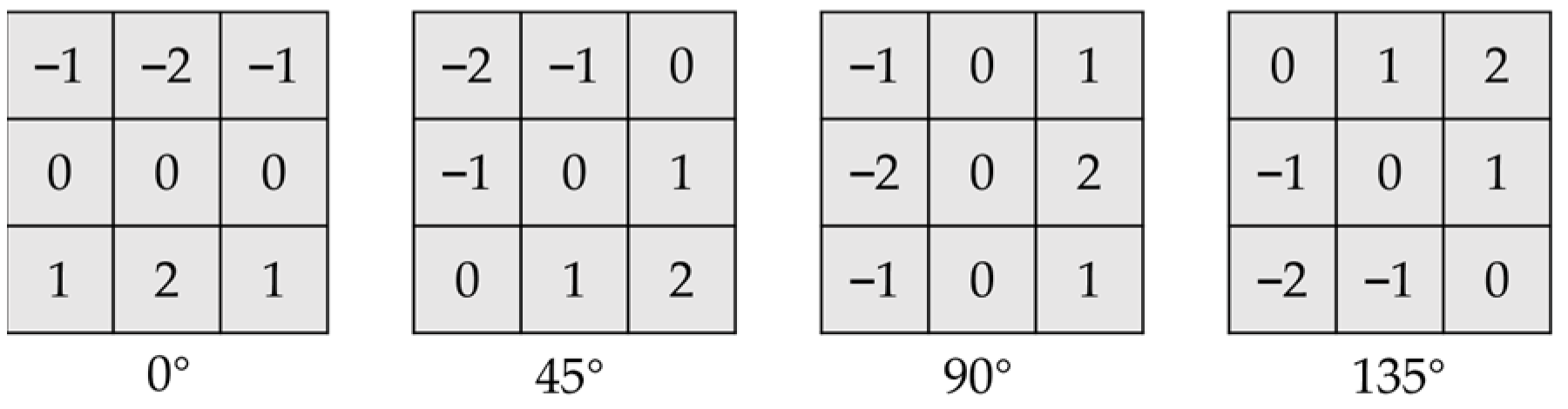
2.3. Adaptive Threshold Sobel Operator

As an important edge detection method, Sobel is a discrete first-order difference operator, which calculates the approximation of the first-order gradient magnitude value [31]. The Sobel operator primarily employs two directional templates (0° for horizontal and 90° for vertical edges). To enhance edge detection’s completeness and accuracy in STIs, we introduce additional templates at 45° and 135°, as shown in Figure 7. These four templates are used to perform convolution operations with the image $3*3$ field. The specific calculation method is as follows [32]:

$$\{\begin{array}{l}\left|G_0\right|=|f(x-1,y-1)+2f(x,y-1)+f(x+1,y-1)-f(x+1,y+1)-2f(x,y+1)-f(x-1,y+1)|\\ \left|G_{45}\right|=|2f(x+1,y-1)+f(x+1,y)+f(x,y-1)-2f(x-1,y+1)-f(x-1,y)-f(x,y+1)|\\ \left|G_{90}\right|=|f(x+1,y+1)+2f(x+1,y)+f(x+1,y-1)-f(x-1,y+1)-2f(x-1,y)-f(x-1,y-1)|\\ \left|G_{135}\right|=|2f(x+1,y+1)+f(x+1,y)+f(x,y+1)-f(x-1,y)-f(x,y-1)-2f(x-1,y-1)|\end{array}$$

(4)

To improve computational efficiency, the sum of absolute values is used to replace the original square and square root operations. The gradient magnitude of a point $(x,y)$ in the image distribution $f(x,y)$ is calculated by the following equation:

$$|\nabla f(x,y)|=\left|G_0\right|+\left|G_{45}\right|+\left|G_{90}\right|+\left|G_{135}\right|$$

(5)

After calculating the gradient magnitude by Equation (5), the traditional Sobel operator performs edge extraction by comparing the magnitude with a fixed threshold $Th$. Specifically, a pixel is classified as an edge point if its gradient magnitude exceeds $Th$; otherwise, it is discarded. This thresholding operation can be expressed as

$$g(x)=\{\begin{array}{l}1,|\nabla f(x,y)>Th|\\ 0,|\nabla f(x,y)\le Th|\end{array}$$

(6)

The selection of an appropriate threshold is crucial for optimal edge detection performance. An excessively low threshold tends to produce false edges by misidentifying noise components, while an overly high threshold may suppress legitimate weak edges, leading to fragmented edge contours. Aiming at this problem, a threshold adaptive algorithm is used to determine the threshold. The procedure of the algorithm is to set a matrix of $3*3$ to move smoothly in an STI with the size of $M*N$. The value of the adaptive threshold $Th$ is determined by calculating the gray average of the pixel values in the $3*3$ matrix in the image. The calculation equation is as follows ($P$ is the pixel gray value in the $3*3$ matrix slider):

$$Th={\displaystyle \frac{1}{9}}(P11+P12+P13+P21+P22+P23+P31+P32+P33)$$

(7)

Since the pixel gray value in the matrix is constantly changing, the calculated threshold is also changing. Each threshold is compared based on the average value in the matrix and the gradient magnitude at the center of the matrix, as shown below:

$$g(x,y)=\{\begin{array}{}\\ 1,|\nabla f(x,y)|>Th\\ X,0.5\cdot Th\le |\nabla f(x,y)|\le Th\\ 0,|\nabla f(x,y)|<0.5\cdot Th\end{array}$$

(8)

If the gradient magnitude of the central pixel is less than half of the adaptive threshold, the point is judged as a non-edge point and the output 0; if the gradient magnitude value is greater than $Th$, it is judged as an edge point and the output 1; if the gradient magnitude is between $0.5*Th$ and $Th$ while the previous point is an edge point, then this point is also an edge point; otherwise, it is not. The Sobel edge detection algorithm based on the adaptive threshold and the traditional Sobel algorithm are used to process the STI. The results are shown in Figure 8. The Sobel edge detection algorithm based on the adaptive threshold is clearer and complete. Edge detection enhances texture gradient representation in STIs, while preserving essential features and suppressing irrelevant noise, thereby achieving effective data compression.

3. Model Training and Fusion Coefficient Determination

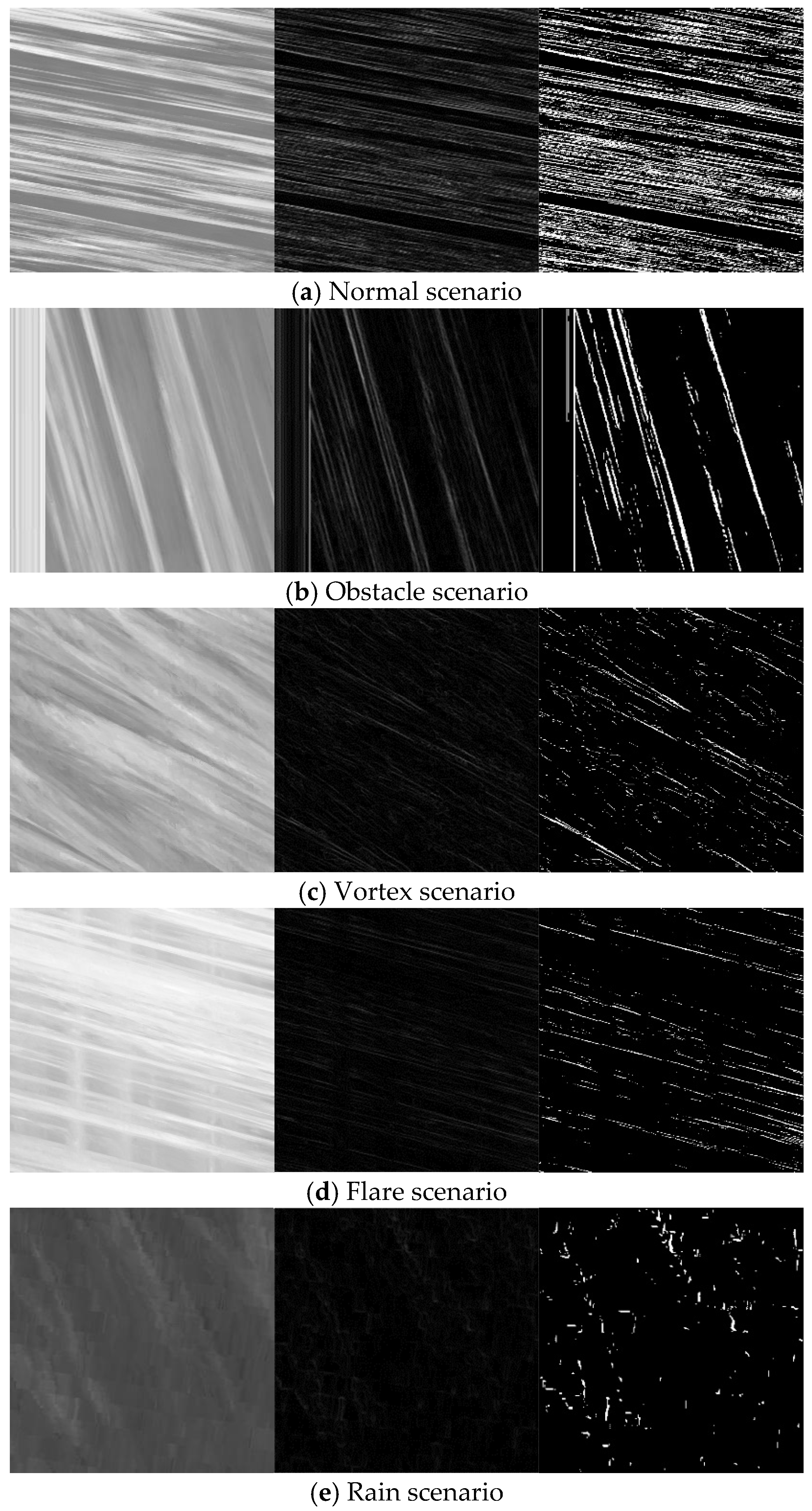
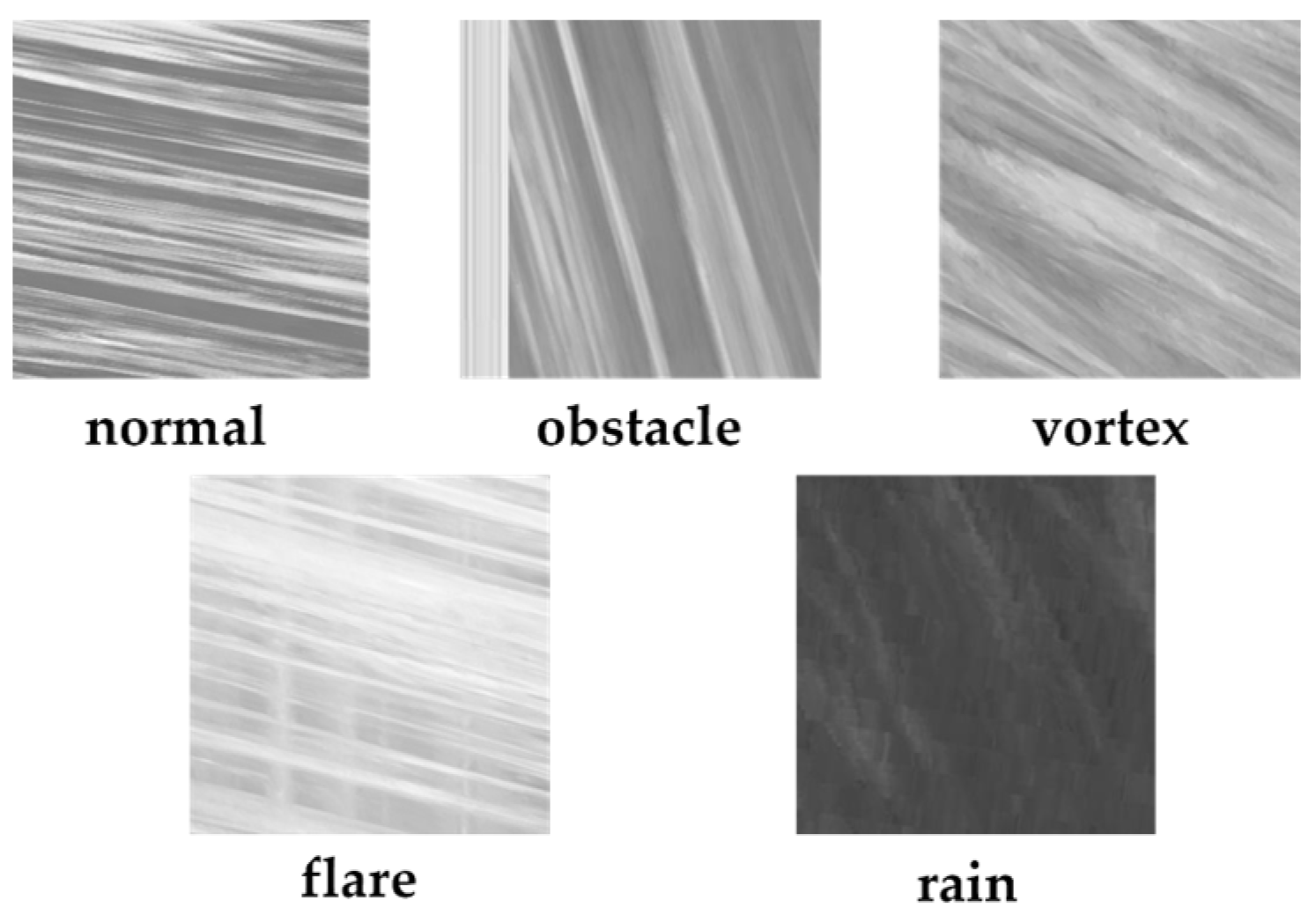
3.1. Dataset Construction

The dataset plays a key role in the training of the model. The quality of the dataset often directly affects the final performance of the model. Given the lack of STI datasets with a wide range and high-precision texture, the video flow measurement system built in the hydrological station collects STIs under different illumination and water flow meteorological conditions and constructs the Panzhihua hydrological station dataset. Panzhihua hydrological station is located in Panzhihua City, Sichuan Province. It is an important national hydrological station, equipped with a hydrological cableway and comprehensive flow measurement facilities. The riverbed is characterized by a large amount of gravel, which is typical of a mountain riverbed. Unlike the gentle silt-laden rivers of the plains, the water here flows turbulently, crashing against rough rocks and forming waves and swirling patterns. These natural flow tracers provide ideal conditions for image-based flow measurement. The flow measurement section is shown in Figure 9a. The video flow measurement system is installed on the side slope of the station on the right bank of the river, as shown in Figure 9b. The corresponding starting distance is 2.9 m, the elevation is 1007.8 m, and the pitch angle is 19.8°. The above calibration parameters are used for the calibration of the river surface flow field without image control. The section monitored by the hydrological station is a relatively stable “U”-shaped profile, with both banks composed of boulders, as shown in Figure 9c. No dams exist downstream of the station. The cross-section shows good control, maintaining a stable stage–discharge single curve for decades. The surface velocity demonstrates a consistent correlation with the sectional discharge.

Data were collected over one year (July 2020 to August 2021) through the online video flow measurement system. The length of the testing line was set to 750 pixels; the duration of the video was 30 s, 25 frames per second; and the size of the synthesized STI was $750*750$ pixels. To make the Panzhihua station dataset cover the various scenarios of real rivers, the dataset was constructed by selecting STIs of five common scenarios, including normal, vortex, flare, obstacles, and rain, as shown in Figure 10. A total of 150 STIs in normal scenarios were selected, of which 100 were used to construct the training set and 50 were used for the test set. In the other four scenarios, 70 STIs were selected, of which 50 were used to construct the training set and the rest were used for the test set. Because the STIs of the normal scenario appear frequently in the actual measurement, the STIs of this scenario account for a large proportion of the dataset. The process of MOT labeling (Figure 11) is as follows: Firstly, a two-dimensional discrete Fourier transform is applied to convert the STI into the frequency domain, where texture related to river tracers manifests as inclined energy concentration lines in the magnitude spectrum. Then, a line segment parallel to the effective energy line is artificially set in the magnitude spectrum. The slope is calculated according to the coordinates $(x_1,y_1)$ and $(x_2,y_2)$ of the two endpoints of the line segment. The main orientation ${\theta }_m$ of the spectrum is obtained:

$${\theta }_m=\arctan ((y_2-y_1)/(x_2-x_1))+90°$$

(9)

Finally, the MOT is obtained according to the orthogonal relationship between the MOT and ${\theta }_m$.

To obtain a dataset with the MOTs showing a wide range of textures, the dataset is expanded by data enhancement. According to the range of the MOTs, the angle values of 168 integers are 5–88 degrees and 92–175 degrees. The STIs of various MOTs are obtained by rotation. The angle step is 1° when rotating. Each STI can be rotated to obtain 168 STIs of the MOT, and the size of the rotated STI is cut to be the same, all of which are $224*224$ pixels. The final Panzhihua station dataset is shown in

Table 1. Composition of Panzhihua dataset.

Scenario	Training Set (Piece)	Test Set (Piece)
normal	16,800	8400
vortex	8400	3360
flare	8400	3360
obstacle	8400	3360
rain	8400	3360

. The total number of images in the training set is 50,400, and the number of test sets is 21,840.

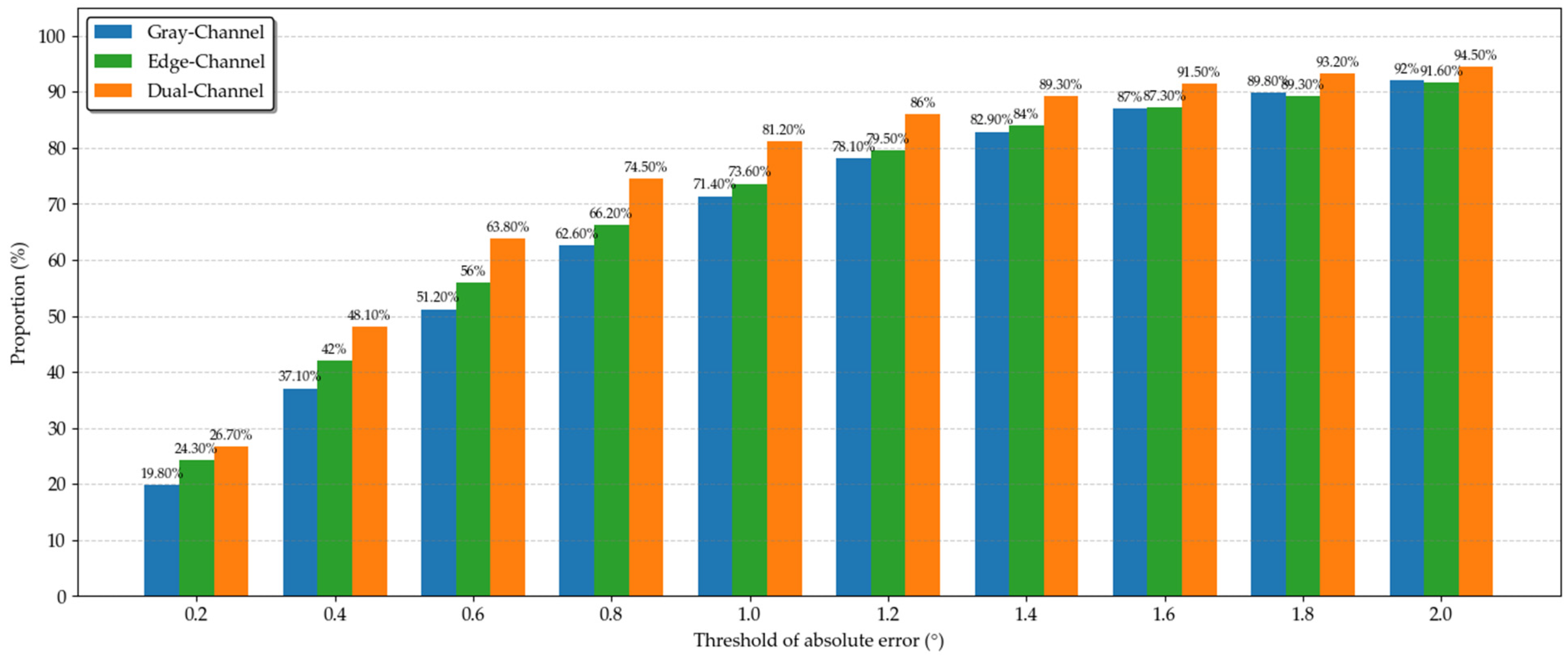
3.2. Determination of Fusion Coefficient

Multiple sets of experiments are performed on the Panzhihua station dataset to investigate the influence of the fusion coefficient $\alpha$ on the model’s detection accuracy. The coefficient is systematically varied from 0 to 1 in 0.1 increments, with $\alpha =1$ corresponding to exclusive use of the Gray-Channel and $\alpha =0$ representing pure Edge-Channel processing. The model’s detection accuracy is quantified using the Mean Absolute Error (MAE), which is calculated as follows:

$$MAE={\displaystyle \frac{1}{N}}{\displaystyle \sum _{i=1}^N|x_i-X_i|}$$

(10)

where $x_i$ is the predicted value estimated by the model, and $X_i$ is the label value. The MAE results corresponding to different fusion coefficients are shown in Figure 12. It can be seen that the MAE with $\alpha =1$ is less than the corresponding MAE with $\alpha =0$, indicating that for MOT detection, the contribution of the original STI is greater than the STI after Sobel detection. $\alpha$ has a small MAE between 0.2 and 0.8. When $\alpha =0.7$, the curve has the lowest point, indicating that the model can achieve the best detection accuracy, and the fusion of these two features in this ratio can obtain the most effective features. Therefore, the value of $\alpha$ is set to 0.7.

4. Experiments and Discussions

4.1. Experimental Platform and Evaluation Method

Experimental platform hardware information: Intel (R) Xeon (R) Gold 5218 CPU @ 2.30 GHz, Quadro RTX 400 graphics card, 8 GB graphics memory, 93.1 GB memory. The software information is as follows: operating system Ubuntu 18.04, programming language Python3.6, deep learning framework Pytorch1.5.1. The hyperparameters in the experiment are set as follows: the initial learning rate is 0.001, the sample size batch size calculated in each iteration is 64, and the number of iteration epochs is 200. The MAE and Standard Deviation (SD) are used as evaluation indicators [33], and the equation of SD is as follows:

$$SD=\sqrt{{\displaystyle \frac{1}{N}}{\displaystyle \sum _{i=1}^n{(y_i-\mu )}^2}}$$

(11)

where $y_i$ is the absolute error of the model prediction, and $\mu$ is the overall average absolute error of the prediction results.

4.2. MOT Detection Comparison Experiments

A comparison is conducted between the dual-channel network and single-channel networks (Gray-Channel and Edge-Channel).

Table 2. MAE and SD results of 3 models on Panzhihua dataset (°).

Regression Model	Dual-Channel	Edge-Channel	Gray-Channel
MAE	0.64	0.87	0.82
SD	0.71	1.01	1.43

and

Table 3. MAE results of 3 models under different scenarios (°).

Scenario	Dual-Channel	Edge-Channel	Gray-Channel
normal	0.41	0.61	0.65
vortex	1.10	1.14	1.15
flare	0.57	0.81	0.82
obstacle	0.33	0.34	0.44
rain	1.17	1.50	1.36

give the MAE and SD for the three models. The overall MAE of Gray-Channel is 0.05° lower than that of Edge-Channel, while it exhibits a 0.42° higher SD. These results suggest that although Gray-Channel provides a slightly higher average accuracy, its detection results are more volatile. In contrast, Edge-Channel achieves a better trade-off between accuracy and robustness. Analyzing Table 3, Edge-Channel outperforms Gray-Channel in normal, obstacle, flare, and vortex scenarios, indicating that the STIs with Sobel detection can obtain more prominent features related to the MOT. So it is easier for the model to learn effective texture features. However, in the rain scenario, the texture features of some STIs are highly blurred. The edge information is not obvious, resulting in the loss of texture features after Sobel detection and the high MAE of Edge-Channel. The proposed Dual-Channel demonstrates better detection accuracy compared to the single-channel models. Specifically, Dual-Channel achieves a 0.18° reduction in MAE relative to Gray-Channel, representing a 21.9% improvement in detection accuracy. This enhancement is consistently observed across all the tested scenarios. The performance gain suggests that the weighted fusion of two channels effectively obtains the features conducive to MOT detection, thereby optimizing DCResNet’s detection capability. Furthermore, the smaller SD of the Dual-Channel model indicates greater stability in detection performance, with the narrowest fluctuation range in absolute error distribution.

To comprehensively demonstrate the detection accuracy of different models, the absolute errors of the three models under the Panzhihua dataset are statistically analyzed according to the threshold. The results are presented in Figure 13, illustrating the proportion of STIs with MOT detection result errors below the specified threshold of absolute error. Overall, Dual-Channel demonstrates good performance, with 94.5% of its detection results maintaining absolute errors below 2°, which is higher than the other two single-channel models, indicating that DCResNet has fewer gross errors and better stability.

4.3. Surface Velocity Comparison Experiments

4.3.1. Experimental Settings of Surface Velocity Measurement

To test the effectiveness of DCResNet applied to noisy scenarios, we select river videos under sunny and rainy weather conditions for surface velocity experiments. The video data used in the experiments are from Panzhihua hydrological station. DCResNet is compared with the FFT method and the manual labeling method. The integration radius of the FFT method is half of the STI size. In addition, an experiment is conducted at the Hebian hydrological station to explore the applicability of DCResNet on other rivers. The FFT, DCResNet, and manual labeling results are all MOT, and the river surface velocity is calculated by Equation (1) based on the corresponding MOT results. Absolute Error (AE), Relative Error (RE), and Mean Relative Error (MRE) are used as evaluation indicators, and the equations are as follows:

$$AE=|z_i-{\widehat{z}}_i|$$

(12)

$$RE=\left|{\displaystyle \frac{z_i-{\widehat{z}}_i}{{\widehat{z}}_i}}\right|$$

(13)

$$MRE={\displaystyle \frac{1}{N}}{\displaystyle \sum _{i=1}^N\left|\frac{z_i-{\widehat{z}}_i}{{\widehat{z}}_i}\right|}$$

(14)

where $z_i$ is the measurement results of the FFT and DCResNet methods, and ${\widehat{z}}_i$ is the corresponding reference values.

4.3.2. Test 1: Sunny Day at Panzhihua Station

The collection time of the river video under sunny conditions is 9 a.m. on 29 July 2020, and the duration of the video is 30 s, as shown in Figure 14. The flow direction of the river is from left to right. The flow tracing conditions are disturbed by many factors, such as vortex, obstacle, and flare. The most obvious interference factor is flare. The cross-section of the flow measurement is a rectangular frame area. Nine testing lines with a starting distance from 45 m to 160 m were measured, including vortex (1, 8, 9), obstacle (1), normal (2–5), and flare (6–9) scenarios. The corresponding STIs are shown in Figure 15.

The MOT and surface velocity results obtained by the three methods are shown in

Table 4. MOT detection results under sunny conditions.

Number	Starting Distance (m)	FFT (°)	DCResNet (°)	Label Value (°)	AE (°)
					FFT	DCResNet
1	45	81.45	80.30	80.89	0.56	0.59
2	65	81.97	82.22	82.20	0.23	0.02
3	75	80.57	80.63	80.80	0.23	0.17
4	85	80.01	80.35	80.48	0.47	0.13
5	95	78.95	78.62	78.80	0.15	0.18
6	115	77.39	77.48	77.52	0.13	0.04
7	130	75.43	74.56	74.45	0.98	0.11
8	145	68.10	66.30	66.10	2.00	0.20
9	160	18.55	41.50	43.39	24.84	1.89

and

Table 5. Surface velocity results under sunny conditions.

Number	Starting Distance (m)	FFT (m/s)	DCResNet (m/s)	Label Value (m/s)	RE (%)
					FFT	DCResNet
1	45	2.48	2.18	2.33	6.44	6.44
2	65	3.91	4.05	4.03	2.98	0.50
3	75	3.92	3.94	4.01	2.24	1.75
4	85	4.15	4.30	4.36	4.82	1.38
5	95	4.16	4.04	4.11	1.22	1.70
6	115	4.29	4.32	4.34	1.15	0.46
7	130	4.20	3.95	3.92	7.14	0.77
8	145	3.08	2.96	2.79	10.39	6.09
9	160	0.44	1.15	1.25	64.8	8.00

. Label values are used as a reference. The label values in Table 4 are the MOT results obtained using the manual labeling method in Section 3.1, and the label values in Table 5 are the surface velocity results calculated by the corresponding MOT. From the MOT detection results in Table 4, the AE on testing lines 2–7 is the smallest, while that of testing lines 1, 8, and 9 is larger. Testing line 1 is located in the near field, which is affected by the near-field vortex and the occlusion of the pipeline, so the detection error of the two methods is slightly larger. Testing lines 2–5 are less disturbed, the textures are clear, and the orientations are consistent. The interference caused by the flare is superimposed in the vertical orientation of testing lines 6 and 7, but the overall texture feature is still obvious. Therefore, FFT and DCResNet can give a more accurate MOT for the STIs corresponding to the testing lines 2–7. Testing lines 8 and 9 are affected by flare and vortex, resulting in a sharp decline in the texture clarity of the STI. The AEs of the FFT method are 2° and 24.84°, respectively, which shows large errors. However, DCResNet can extract effective texture features and has a certain degree of robustness to noise by training on the Panzhihua dataset, which gives a more reliable MOT detection. The AE of the MOT is controlled within 2°.

The corresponding surface velocity distribution is shown in Figure 16. Overall, the surface velocity results obtained by DCResNet are closer to the label values, and the MRE is 3.01%, which has good robustness. However, in the scenario disturbed by multiple noises, the detection results of FFT have a large deviation, which leads to unreliable surface velocity values.

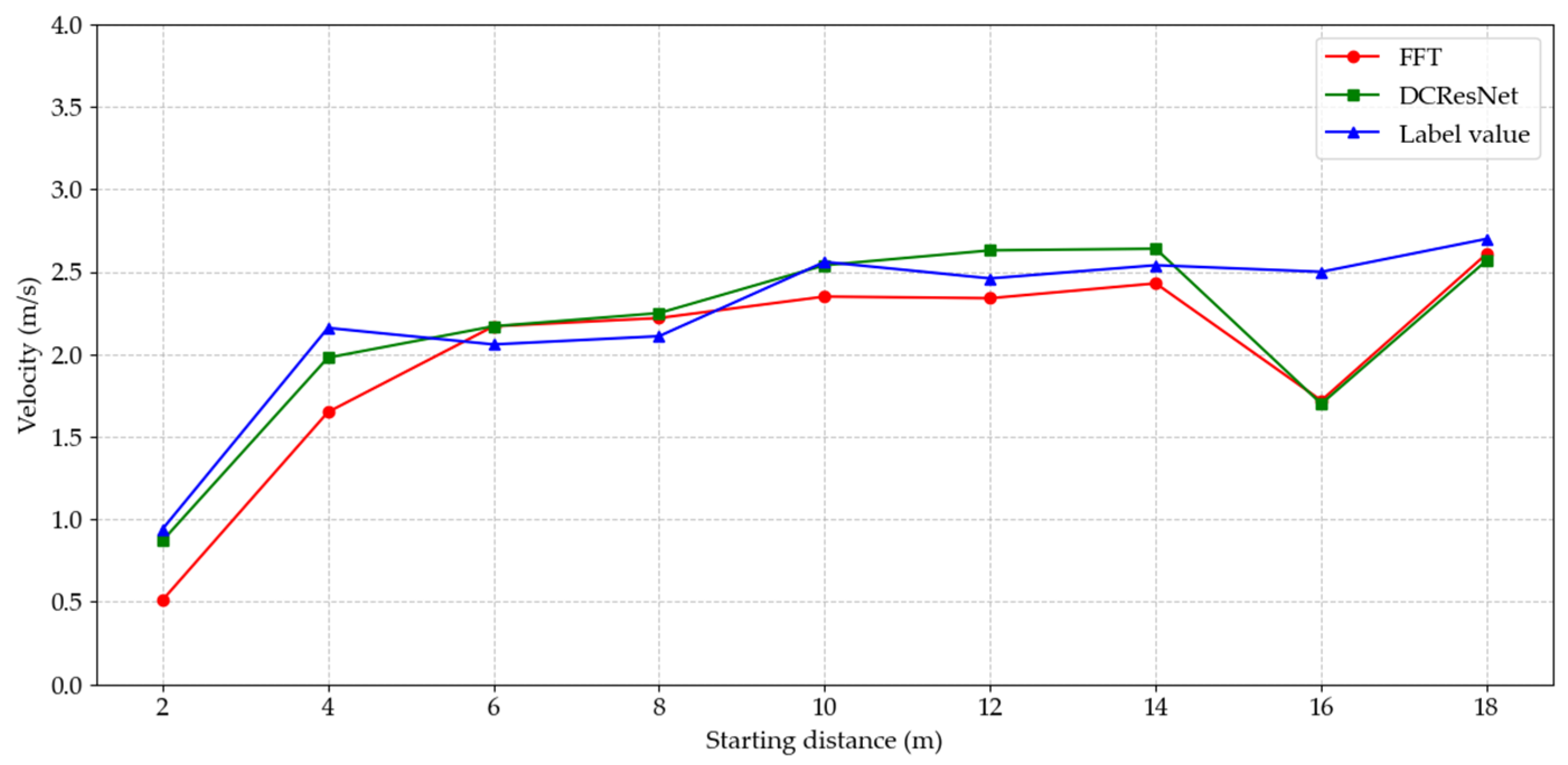
4.3.3. Test 2: Rainy Day at Panzhihua Station

The river video is captured at 9:00 on 24 August 2020, under rainy conditions. The river cross-section is shown in Figure 17. The current shooting conditions are harsh; the light is dim and affected by rain. The visibility of water flow tracers is poor, measuring nine testing lines from a starting distance of 50 m to 160 m. It mainly includes vortex (1, 8, 9) and rain (1–9) scenarios. The corresponding STIs are shown in Figure 18.

The results of MOT and surface velocity obtained are shown in

Table 6. MOT detection results under rainy conditions.

Number	Starting Distance (m)	FFT (°)	DCResNet (°)	Label Value (°)	AE (°)
					FFT	DCResNet
1	50	23.95	77.11	78.02	54.07	0.91
2	60	80.44	79.69	80. 01	0.43	0.32
3	75	80.42	80.62	80.78	0.36	0.16
4	85	79.31	78.60	78.31	1.00	0.29
5	95	78.50	79.03	78.75	0.25	0.28
6	105	77.02	77.39	77.21	0.19	0.18
7	120	74.55	75.02	74.68	0.13	0.34
8	140	76.12	67.59	65.34	10.78	2.25
9	160	23.30	39.12	37.25	13.95	1.87

and

Table 7. Surface velocity results under rainy conditions.

Number	Starting Distance (m)	FFT (m/s)	DCResNet (m/s)	Label Value (m/s)	RE (%)
					FFT	DCResNet
1	50	0.20	2.06	2.21	90.95	6.79
2	60	3.28	3.04	3.16	3.80	3.80
3	75	3.66	3.75	3.81	3.94	1.57
4	85	3.69	3.47	3.37	9.50	2.97
5	95	3.92	4.12	4.01	2.24	2.74
6	105	3.80	3.93	3.87	1.81	1.55
7	120	3.71	3.84	3.74	0.80	2.67
8	140	4.75	2.85	2.56	85.55	11.33
9	160	0.56	1.06	0.99	43.43	7.07

. Notably, at the testing lines (1, 8, 9), the STIs suffer from severe texture degradation due to rain and vortex interference. This dual disturbance manifests as both feature blurring and an inconsistent texture orientation. For the FFT, which depends on texture clarity, the less effective texture features result in AEs of 54.07°, 10.78°, and 13.95° in the MOT detection results. The results underscore the challenge of frequency-domain analysis under poor texture conditions. DCResNet demonstrates robust performance under challenging conditions due to its enhanced feature extraction capability. Although the texture features are weak, DCResNet can still extract effective texture features and then learn the complex nonlinear mapping function from texture features to angle space. This enables accurate MOT detection, with the AE constrained below 2.25°.

Figure 19 shows the surface velocity distribution. It can be seen that the FFT and DCResNet surface velocity distributions on the testing lines (2–7) with better tracer conditions are close to the label values. At this time, the RE of the surface velocity of DCResNet can be controlled within 3.80%. For testing lines (1, 8, 9), which are greatly affected by noise, the surface velocity results of FFT show abnormal values, while DCResNet can give more accurate velocity values. The MRE of DCResNet in this test is 4.50%, which is 22.39% less than FFT, verifying the robustness of DCResNet in noisy scenarios.

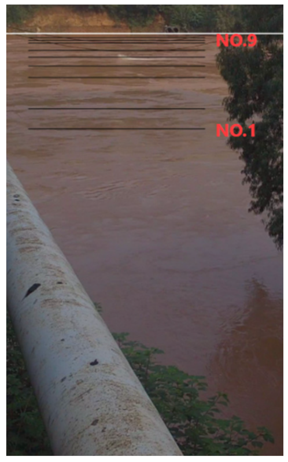
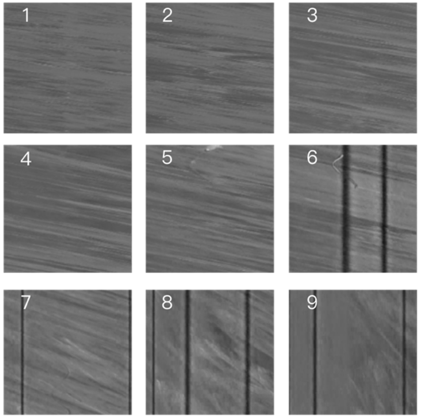
4.3.4. Test 3: Cloudy Day at Hebian Station

To test the applicability of DCResNet to other rivers, a comparative experiment was conducted at the Hebian hydrological station in Qujing City, Yunnan Province, which monitors a typical medium-sized river in mountainous areas. The river video of this test was captured at 10:50 on 30 May 2022, during the high flood period with cloudy conditions. The river cross-section is shown in Figure 20. Unlike the two tests in Panzhihua station, the river flows from right to left, and there are more waves on the river surface. A total of nine testing lines were measured, with a starting distance of 2 m to 18 m. The corresponding STIs are shown in Figure 21.

The MOT and surface velocity results are listed in

Table 8. MOT detection results of Hebian station.

Number	Starting Distance (m)	FFT (°)	DCResNet (°)	Label Value (°)	AE (°)
					FFT	DCResNet
1	2	81.30	84.87	85.24	3.94	0.37
2	4	85.49	86.24	86.56	1.07	0.32
3	6	86.66	86.65	86.47	0.19	0.18
4	8	86.11	86.15	85.9	0.21	0.25
5	10	85.69	86.02	86.05	0.36	0.03
6	12	85.07	85.61	85.31	0.24	0.30
7	14	84.66	85.10	84.91	0.25	0.19
8	16	81.75	81.65	84.32	2.57	2.67
9	18	83.67	83.56	83.88	0.21	0.32

and

Table 9. Surface velocity results of Hebian station.

Number	Starting Distance (m)	FFT (m/s)	DCResNet (m/s)	Label Value (m/s)	RE (%)
					FFT	DCResNet
1	2	0.51	0.87	0.94	45.74	7.45
2	4	1.65	1.98	2.16	23.61	8.33
3	6	2.17	2.17	2.06	5.34	5.34
4	8	2.22	2.25	2.11	5.21	6.64
5	10	2.35	2.54	2.56	8.20	0.78
6	12	2.34	2.63	2.46	4.88	6.91
7	14	2.43	2.64	2.54	4.33	3.94
8	16	1.72	1.7	2.50	31.20	32.00
9	18	2.61	2.57	2.70	3.33	4.81

, respectively. At testing line 1, the camera captures fewer flow features and is accompanied by obstacle interference, which manifests as feature ambiguity in the corresponding STI. The AE of FFT is 3.94°, while that of DCResNet is only 0.37°. The corresponding RE of DCResNet is reduced by 38.29% compared with FFT. In addition, at testing line 8, due to the significant interference of river waves, the consistency of the STI texture is weakened. The AEs of FFT and DCResNet are 2.57° and 2.67°, respectively. The corresponding RE reaches as high as 31.20% and 32.00%. This occurs because the Panzhihua dataset used to train DCResNet does not include STI samples with wave scenarios, which limits the detection accuracy of DCResNet in such conditions. Therefore, expanding the diversity of the dataset to improve the generalization ability of DCResNet can be a focus of future research.

The corresponding surface velocity distribution is shown in Figure 22. Overall, the surface velocity results obtained by DCResNet are closer to the label values than those obtained by FFT. Except for the uncovered wave scenario at test line 8, DCResNet achieves an MRE of 5.53%, representing a 7.05% reduction compared to FFT. These results demonstrate the model’s good applicability to the Hebian station.

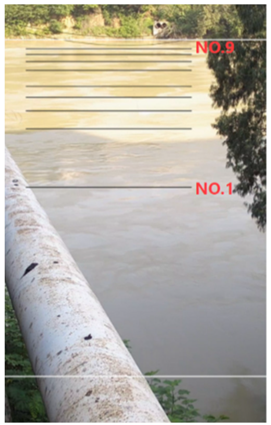
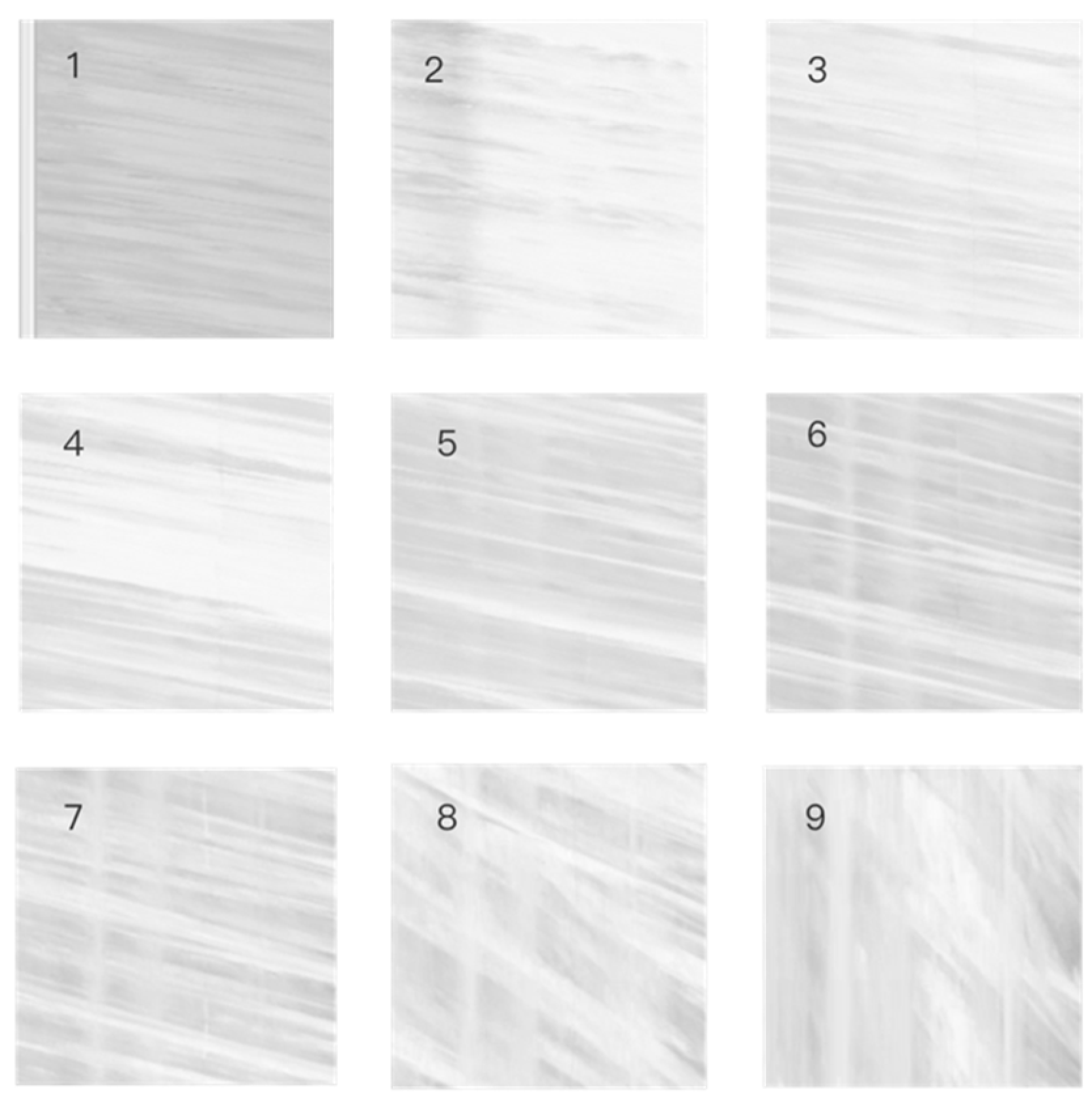
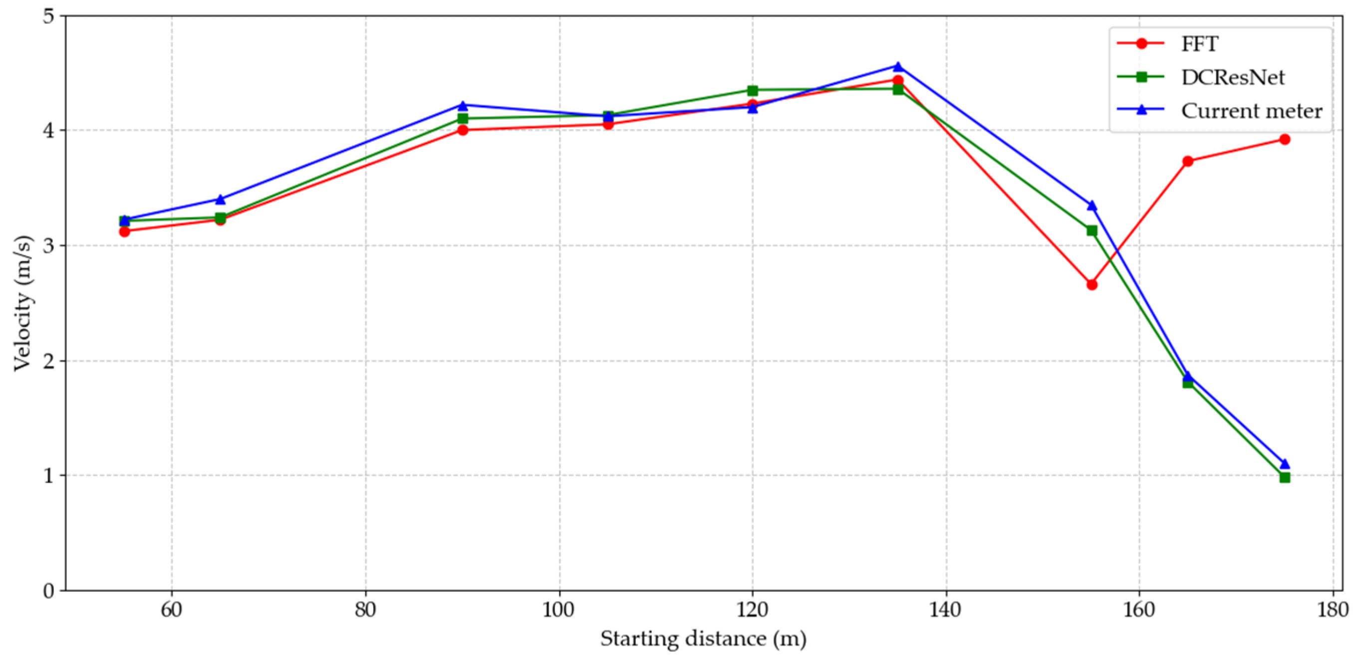
4.4. Vertical Average Velocity Comparison Experiment

4.4.1. Experimental Settings of Vertical Average Velocity Measurement

In China’s current hydrological measurement system, the velocity and discharge measured by the current meter are considered true values, which is the standard for evaluating the accuracy of various new flow measurement methods. So, to assess the practical performance of DCResNet, a comparative experiment with current meter measurements is conducted at the Panzhihua hydrological station. The current meter model used is LS25-3A. Since the current meter cannot precisely measure surface velocity, the vertical average velocity is used for comparison, following references [18,25,34]. The specific experimental method is as follows: during the video shooting, simultaneous measurements are taken with the current meter to ensure synchronized data collection. For the current meter method, measurement vertical lines are set at 55 m, 65 m, 90 m, 105 m, 120 m, 135 m, 155 m, 165 m, and 175 m from the starting point, respectively. At each vertical line, velocities are measured by the current meter at relative depths (the ratio between the depth of the measuring point and the depth of the vertical line) of 0.2 and 0.8, with their average representing the vertical average velocity. Based on the current meter’s position in the video, testing lines are set at the same locations. After obtaining surface velocities via the FFT and DCResNet method, they are multiplied by a velocity coefficient to derive the corresponding vertical average velocity. The velocity coefficient is derived from historical statistical data at the hydrological station, which is defined as the ratio of measured discharge to the virtual discharge calculated from the surface velocity. The three indicators AE, RE, and MRE in Section 4.3.1 are still used for error evaluation, with the results of the current meter as reference values.

4.4.2. Experimental Results

The comparison period is from 8:25 to 9:25 on 21 August 2020. As shown in Figure 23, the water level of the river is maintained at 998 m, which belongs to high water conditions. The corresponding velocity coefficient is 0.89. During this period, the flow tracer and surface velocity are relatively stable. The experiment uses a 30 s video taken at 9:00 to measure nine testing lines from 55 m to 175 m, including normal (2–5), vortex (1, 9), and obstacle (6–9) scenarios. The corresponding STIs are shown in Figure 24.

The obtained MOT and vertical average velocity results are listed in

Table 10. MOT detection results.

Number	Starting Distance (m)	FFT (°)	DCResNet (°)	Label Value (°)	AE (°)
					FFT	DCResNet
1	55	82.71	82.91	82.60	0.11	0.31
2	65	81.66	81.72	81.54	0.12	0.18
3	90	80.61	80.83	80.69	0.08	0.14
4	105	79.32	79.53	79.40	0.08	0.13
5	120	78.18	78.52	78.38	0.20	0.14
6	135	77.55	77.32	77.41	0.14	0.09
7	155	73.10	70.21	69.81	3.29	0.40
8	165	70.52	58.45	56.80	13.72	1.65
9	175	72.02	37.69	38.20	33.82	0.51

and

Table 11. Vertical average velocity results.

Number	Starting Distance (m)	FFT (m/s)	DCResNet (m/s)	Current Meter (m/s)	RE (%)
					FFT	DCResNet
1	55	3.12	3.21	3.22	3.11	0.31
2	65	3.22	3.24	3.40	5.29	4.71
3	90	4.00	4.10	4.22	5.21	2.84
4	105	4.05	4.13	4.12	1.70	0.24
5	120	4.23	4.35	4.20	0.71	3.57
6	135	4.44	4.36	4.56	2.63	4.39
7	155	2.66	3.13	3.35	20.60	6.57
8	165	3.73	1.81	1.87	99.47	3.21
9	175	3.92	0.98	1.10	256.36	10.91

, respectively. Table 10 reveals that the AE is minimized under the normal scenario, whereas higher AE values are observed in both obstacle and vortex scenarios. Analysis of each STI reveals that while testing line 1 experiences vortex interference, its effective texture features remain distinct. Similarly, testing lines 5–6, despite partial occlusion by the current meter and black cable, maintain clear and consistent tracer-generated textures. Consequently, both the FFT and DCResNet methods demonstrate accurate MOT detection for testing lines 1–6. However, testing lines 7–9 present greater challenges due to concurrent cable obstruction and far-bank vortex effects, leading to texture blurring, inconsistent flow directionality, and multi-oriented interference patterns. Furthermore, testing line 9 suffers from reduced resolution owing to its far-field position. These factors cause substantial FFT-derived deviations (3.29–33.82°, maximized at line 9), whereas DCResNet maintains better performance through robust texture feature extraction. By ensuring a reliable MOT estimation, DCResNet consistently limits the AE below 2°, effectively preventing the gross errors observed in the FFT results.

Figure 25 presents the vertical average velocity distribution, revealing distinct performance characteristics between the two methods. In the 55–135 m range, both FFT and DCResNet demonstrate good agreement with the current meter measurements, maintaining an RE below 6%. However, significant differences emerge in the 155–175 m section, where vortex and obstacle interference become more pronounced. In this region, the FFT results exhibit abnormal fluctuations, with an exceptionally high RE of 256.36%, demonstrating the method’s failure under these challenging conditions. In contrast, DCResNet successfully mitigates gross errors, maintaining a consistent velocity distribution with current meter measurements across the entire 55–175 m range. The method’s MRE of 4.08% further confirms its reliability for practical velocity measurement applications, which is better than the FFT method.

5. Conclusions

This paper proposes a Space–Time Image Velocimetry method based on a dual-channel residual network (DCResNet) through the joint learning of original and edge-enhanced STIs. The method has a dual-channel network structure, where one channel processes the original STI while the other analyzes the STI after adaptive threshold Sobel detection. This edge detection channel enhances texture features, and the weighted fusion of both channels’ outputs feeds into the regression layer for final MOT detection. Experimental results show that DCResNet works best with a 7:3 fusion ratio of original and edge features on the Panzhihua station dataset. It achieves a 0.41° accuracy in normal scenarios and stays within 1.2° in complex noise scenarios. Compared with the single-channel models, DCResNet achieves a lower MAE and SD, while demonstrating enhanced robustness in complex scenarios. In three groups of surface velocity comparison experiments, DCResNet shows better performance than the FFT method. This method exhibited enhanced robustness, especially when processing STIs with weak texture features. Furthermore, it also has good applicability for the river not covered by the STI dataset. The vertical average velocity comparison experiment results show that DCResNet achieves an overall MOT detection AE below 1.65° and an MRE of 4.08%. The velocity distribution is consistent with the current meter results, confirming its practicality for flow velocity monitoring. However, compared to traditional methods, DCResNet requires greater computational resources and a longer training time. In future research, we will explore lightweight models to the reduce computational complexity, while expanding the scenario diversity of the STI dataset (e.g., including wave scenarios) to further improve its detection accuracy.

References

1. Gao, G.; Li, J.; Feng, P.; Liu, J.; Wang, Y. Impacts of climate and land-use change on flood events with different return periods in a mountainous watershed of North China. J. Hydrol. Reg. Stud. 2024, 55, 101943. [Google Scholar] [CrossRef]
2. Perks, M.T.; Sasso, S.F.D.; Hauet, A.; Jamieson, E.; Le Coz, J.; Pearce, S.; Peña-Haro, S.; Pizarro, A.; Strelnikova, D.; Tauro, F.; et al. Towards harmonisation of image velocimetry techniques for river surface velocity observations. Earth Syst. Sci. Data 2020, 12, 1545–1559. [Google Scholar] [CrossRef]
3. Dobriyal, P.; Badola, R.; Tuboi, C.; Hussain, S.A. A review of methods for monitoring streamflow for sustainable water resource management. Appl. Water Sci. 2017, 7, 2617–2628. [Google Scholar] [CrossRef]
4. Jodeau, M.; Hauet, A.; Paquier, A.; Coz, J.L.; Dramais, G. Application and evaluation of LS-PIV technique for the monitoring of river surface velocities in high flow conditions. Flow Meas. Instrum. 2008, 19, 117–127. [Google Scholar] [CrossRef]
5. Coz, J.L.; Hauet, A.; Pierrefeu, G.; Dramais, G.; Camenen, B. Performance of image-based velocimetry (LSPIV) applied to flash-flood discharge measurements in Mediterranean rivers. J. Hydrol. 2010, 394, 42–52. [Google Scholar] [CrossRef]
6. Tsubaki, R.; Fujita, I.; Tsutsumi, S. Measurement of the flood discharge of a small-sized river using an existing digital video recording system. J. Hydro-Environ. Res. 2011, 5, 313–321. [Google Scholar] [CrossRef]
7. Muste, M.; Fujita, I.; Hauet, A. Large-scale particle image velocimetry for measurements in riverine environments. Water Resour. Res. 2008, 44, W00D19. [Google Scholar] [CrossRef]
8. Thumser, P.; Haas, C.; Tuhtan, J.A.; Fuentes-Pérez, J.F.; Toming, G. RAPTOR-UAV: Real-time particle tracking in rivers using an unmanned aerial vehicle. Earth Surf. Process. Landf. 2017, 42, 2439–2446. [Google Scholar] [CrossRef]
9. Tauro, F.; Tosi, F.; Mattoccia, S.; Toth, E.; Piscopia, R.; Grimaldi, S. Optical Tracking Velocimetry (OTV): Leveraging Optical Flow and Trajectory-Based Filtering for Surface Streamflow Observations. Remote Sens. 2018, 10, 2010. [Google Scholar] [CrossRef]
10. Fujita, I.; Watanabe, H.; Tsubaki, R. Development of a non-intrusive and efficient flow monitoring technique: The space-time image velocimetry (STIV). Int. J. River Basin Manag. 2007, 5, 105–114. [Google Scholar] [CrossRef]
11. Tsubaki, R. On the Texture Angle Detection Used in Space-Time Image Velocimetry (STIV). Water Resour. Res. 2017, 53, 10908–10914. [Google Scholar] [CrossRef]
12. Fujita, I.; Kobayashi, K.; Logah, F.Y.; Oblim, F.T.; Alfa, B.; Tateguchi, S.; Kankam-Yeboah, K.; Appiah, G.; Asante-Sasu, C.K.; Kawasaki, R.; et al. Accuracy of Ku-stiv for Discharge Measurement in Ghana, Africa. J. Jpn. Soc. Civ. Eng. Ser. B1 (Hydraul. Eng.) 2017, 73, I_499–I_504. [Google Scholar] [CrossRef]
13. Zhang, Z.; Zhou, Y.; Li, H.; Liu, L. Development and application of an image-based flow measurement system. Water Resour. Inf. 2018, 3, 7–13. [Google Scholar] [CrossRef]
14. Zhen, W.; Chen, H.; Chen, D.; Cai, F.; Fang, W.; Chen, D.; Wang, R.; He, X.; Wang, B.; Guo, L. The Ecological Flow Intelligent Supervision Platform Based on Wuhan University’s AiFlow Visual Flow Measurement Technology and Its Application. J. Water Resour. Res. 2024, 13, 347–354. [Google Scholar] [CrossRef]
15. Hydro-STIV. Available online: https://hydrosoken.co.jp/service/hydrostiv.php (accessed on 25 June 2024).
16. Fujita, I.; Notoya, Y.; Tani, K.; Tateguchi, S. Efficient and accurate estimation of water surface velocity in STIV. Environ. Fluid Mech. 2019, 19, 1363–1378. [Google Scholar] [CrossRef]
17. Zhen, Z.; Huabao, L.; Yang, Z.; Jian, H. Design and evaluation of an FFT-based space-time image velocimetry (STIV) for time-averaged velocity measurement. In Proceedings of the 2019 14th IEEE International Conference on Electronic Measurement & Instruments (ICEMI), Changsha, China, 1–3 November 2019. [Google Scholar]
18. Zhao, H.; Chen, H.; Liu, B.; Liu, W.; Xu, C.-Y.; Guo, S.; Wang, J. An improvement of the Space-Time Image Velocimetry combined with a new denoising method for estimating river discharge. Flow Meas. Instrum. 2021, 77, 101864. [Google Scholar] [CrossRef]
19. Tani, K.; Fujita, I. Wavenumber-frequency analysis of river surface texture to improve accuracy of image-based velocimetry. E3S Web Conf. 2018, 40, 8. [Google Scholar] [CrossRef]
20. Zhang, Z.; Li, H.; Yuan, Z.; Dong, R.; Wang, J. Sensitivity analysis of image filter for space-time image velocimetry in frequency domain. Chin. J. Sci. Instrum. 2022, 43, 43–53. [Google Scholar] [CrossRef]
21. Liu, X.; Li, S.; Kan, M.; Zhang, J.; Chen, X. AgeNet: Deeply Learned Regressor and Classifier for Robust Apparent Age Estimation. In Proceedings of the IEEE International Conference on Computer Vision Workshop, Santiago, Chile, 7–13 December 2015. [Google Scholar]
22. Luo, P.; Tian, Y.; Wang, X.; Tang, X. Switchable Deep Network for Pedestrian Detection. In Proceedings of the Computer Vision & Pattern Recognition, Columbus, OH, USA, 23–28 June 2014; pp. 899–906. [Google Scholar]
23. Zhang, J.; Shan, S.; Kan, M.; Chen, X. Coarse-to-Fine Auto-Encoder Networks (CFAN) for Real-Time Face Alignment. In Proceedings of the Computer Vision—ECCV 2014, Zurich, Switzerland, 6–12 September 2014; Springer: Cham, Switzerland, 2014. [Google Scholar] [CrossRef]
24. Watanabe, K.; Fujita, I.; Iguchi, M.; Hasegawa, M. Improving Accuracy and Robustness of Space-Time Image Velocimetry (STIV) with Deep Learning. Water 2021, 13, 2079. [Google Scholar] [CrossRef]
25. Hu, Q.; Wang, J.; Zhang, G.; Jin, J. Space-time image velocimetry based on improved MobileNetV2. Electronics 2023, 12, 399. [Google Scholar] [CrossRef]
26. Huang, Y.; Chen, H.; Huang, K.; Chen, M.; Wang, J.; Liu, B. Optimization of Space-Time image velocimetry based on deep residual learning. Measurement 2024, 232, 114688. [Google Scholar] [CrossRef]
27. Li, H.; Zhang, Z.; Chen, L.; Meng, J.; Sun, Y. Surface space-time image velocimetry of river based on residual network. J. Hohai Univ. (Nat. Sci.) 2023, 51, 118–128. [Google Scholar] [CrossRef]
28. Guo, Y.; Yang, W.; Liu, Q.; Wang, Y. Survey of residual network. Appl. Res. Comput. 2020, 37, 1292–1297. [Google Scholar] [CrossRef]
29. Xu, Y.; Li, Z.; Li, W.; Du, Q.; Zhai, L. Dual-Channel Residual Network for Hyperspectral Image Classification With Noisy Labels. IEEE Trans. Geosci. Remote Sens. 2021, 60, 5502511. [Google Scholar] [CrossRef]
30. He, K.; Zhang, X.; Ren, S.; Sun, J. Deep Residual Learning for Image Recognition; IEEE: New York, NY, USA, 2016. [Google Scholar] [CrossRef]
31. Israni, S.; Jain, S. Edge detection of license plate using Sobel operator. In Proceedings of the 2016 International Conference on Electrical, Electronics, and Optimization Techniques (ICEEOT), Chennai, India, 3–5 March 2016; pp. 3561–3563. [Google Scholar]
32. Zhai, Q.; Liu, Q.; Zhang, J.; Huang, Y.; Gao, Y. Research and Implementation of Sobel Edge Detection System Based on Smooth Adaptive. In Proceedings of the 17th China Aviation Measurement and Control Technology Annual Conference, Xi’an, China, 5 November 2020. [Google Scholar]
33. Kuo, P.-H.; Huang, C.-J. A High Precision Artificial Neural Networks Model for Short-Term Energy Load Forecasting. Energies 2018, 11, 213. [Google Scholar] [CrossRef]
34. Zhang, Z.; Chen, L.; Yuan, Z.; Gao, L. Validity Identification and Rectification of Water Surface Fast Fourier Transform-Based Space-Time Image Velocimetry (FFT-STIV) Results. Sensors 2025, 25, 257. [Google Scholar] [CrossRef]
Figure 1. STI synthesis.
Applsci 15 05284 g001
Figure 2. STIV based on DCResNet.
Applsci 15 05284 g002
Figure 3. Two-layer identity residual block.
Applsci 15 05284 g003
Figure 4. The structure of DCResNet.
Applsci 15 05284 g004
Figure 5. Structure and parameters of ResNet18 feature extraction layer.
Applsci 15 05284 g005
Figure 6. Structure of Basic Block.
Applsci 15 05284 g006
Figure 7. Direction templates of Sobel operator.
Applsci 15 05284 g007
Figure 8. Results of traditional Sobel and adaptive threshold Sobel. (The left, middle, and right figures are original STIs, the traditional Sobel effect, and the adaptive threshold Sobel effect.)
Applsci 15 05284 g008
Figure 9. Section view and system setup of Panzhihua hydrological station.
Applsci 15 05284 g009
Figure 10. STIs in different scenarios.
Applsci 15 05284 g010
Figure 11. MOT by manual labeling.
Applsci 15 05284 g011
Figure 12. The results of the model’s detection accuracy.
Applsci 15 05284 g012
Figure 13. Absolute error distribution of detection results for 3 models.
Applsci 15 05284 g013
Figure 14. Section diagram of test 1.
Applsci 15 05284 g014
Figure 15. STIs under sunny conditions. (1–9 correspond to the starting distances of 45 m, 65 m, 75 m, 85 m, 95 m, 115 m, 130 m, 145 m, 160 m, respectively.)
Applsci 15 05284 g015
Figure 16. Surface velocity distribution of test 1.
Applsci 15 05284 g016
Figure 17. Section diagram of test 2.
Applsci 15 05284 g017
Figure 18. STIs under rainy conditions. (1–9 correspond to the starting distances of 50 m, 60 m, 75 m, 85 m, 95 m, 105 m, 120 m, 140 m, 160 m, respectively.)
Applsci 15 05284 g018
Figure 19. Surface velocity distribution of test 2.
Applsci 15 05284 g019
Figure 20. Section diagram of test 3.
Applsci 15 05284 g020
Figure 21. STIs under cloudy conditions. (1–9 correspond to the starting distances of 2 m, 4 m, 6 m, 8 m, 10 m, 12 m, 14 m, 16 m, 18 m, respectively.)
Applsci 15 05284 g021
Figure 22. Surface velocity distribution of test 3.
Applsci 15 05284 g022
Figure 23. Section diagram.
Applsci 15 05284 g023
Figure 24. STIs of different testing lines. (1–9 correspond to the starting distances of 55 m, 65 m, 90 m, 105 m, 120 m, 135 m, 155 m, 165 m, 175 m, respectively.)
Applsci 15 05284 g024
Figure 25. Vertical average velocity distribution.
Applsci 15 05284 g025