

Unknown IoT Device Identification Models and Algorithms Based on CSCL-Siamese Networks and Weighted-Voting Clustering Ensemble

Abstract
1. Introduction
- (1)
- An algorithm for generating PNSPs, which establishes a set of PNSPs by combining data visualization techniques with a permutation sample-generation strategy, is proposed. This algorithm ensures that each sample is fully utilized, thus mitigating the issue of reduced identification performance caused by underutilized datasets.
- (2)
- A Siamese network based on cost-sensitive contrastive loss (CSCL-Siamese) is presented. By improving the classical contrastive loss function, using the Manhattan distance as the similarity metric, and leveraging the disparity between counts of positive and negative sample pairs, this approach assigns greater weighting factors to the positive sample pairs to increase their loss cost, thus addressing the issue of decision boundary bias toward negative sample pairs caused by an insufficient number of positive sample pairs.
- (3)
- A UDI algorithm based on a WVE (WVE-UDI) is developed. By combining weighting factors with a voting ensemble strategy, this algorithm integrates the clustering results of multiple unsupervised clustering algorithms, thus overcoming the limitations of individual clustering algorithms and improving the capability for identifying unknown IoT devices.
- (4)
- Finally, the algorithms above are integrated into the CSCL-WVE-UDI method for UDI. Experimental results show that the CSCL-WVE-UDI method can effectively identify multiple types of unknown IoT devices.
2. Literature Review
3. CSCL-WVE-UDI: Method for Identifying Unknown IoT Devices
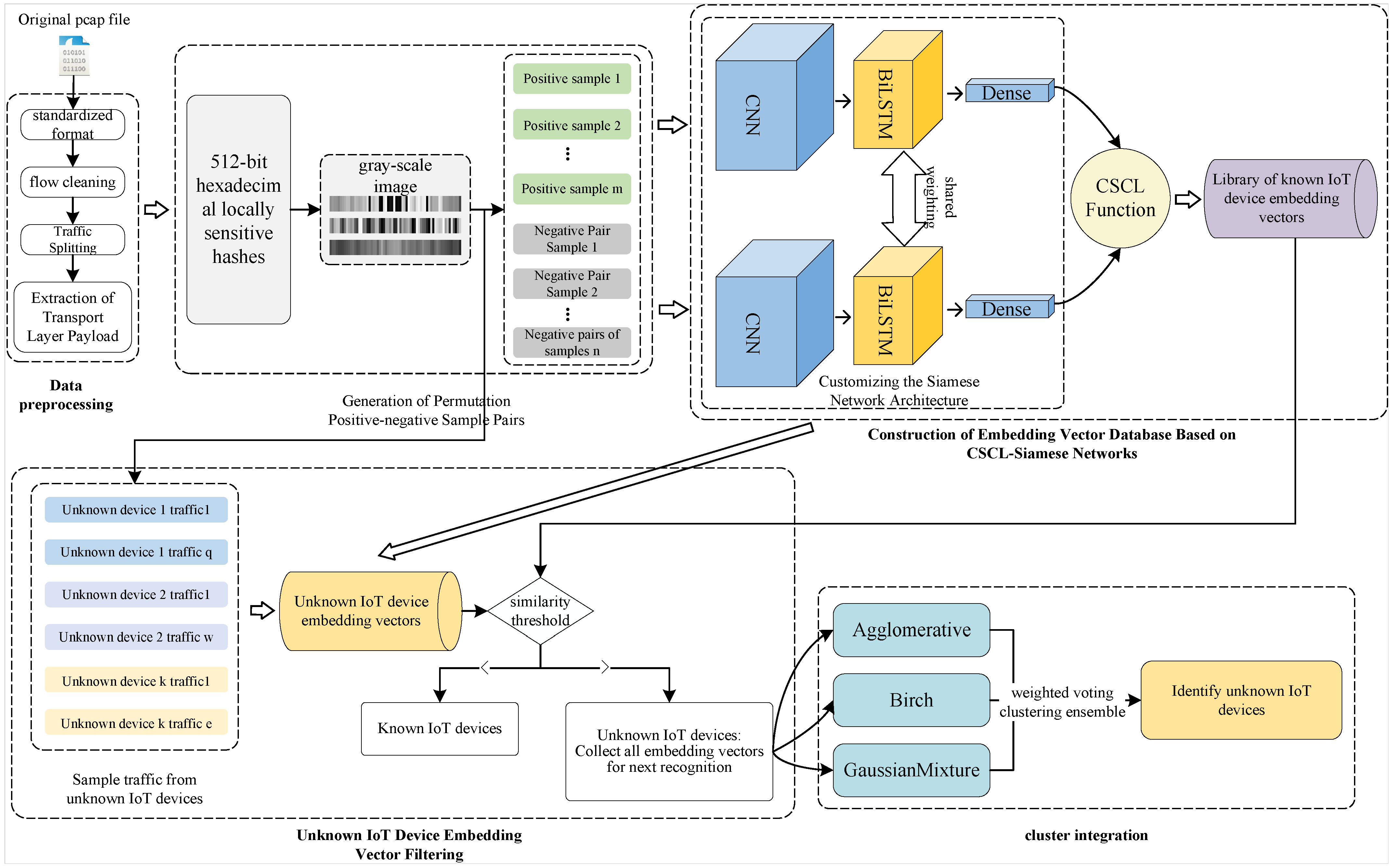
3.1. Logical Architecture of CSCL-WVE-UDI Method
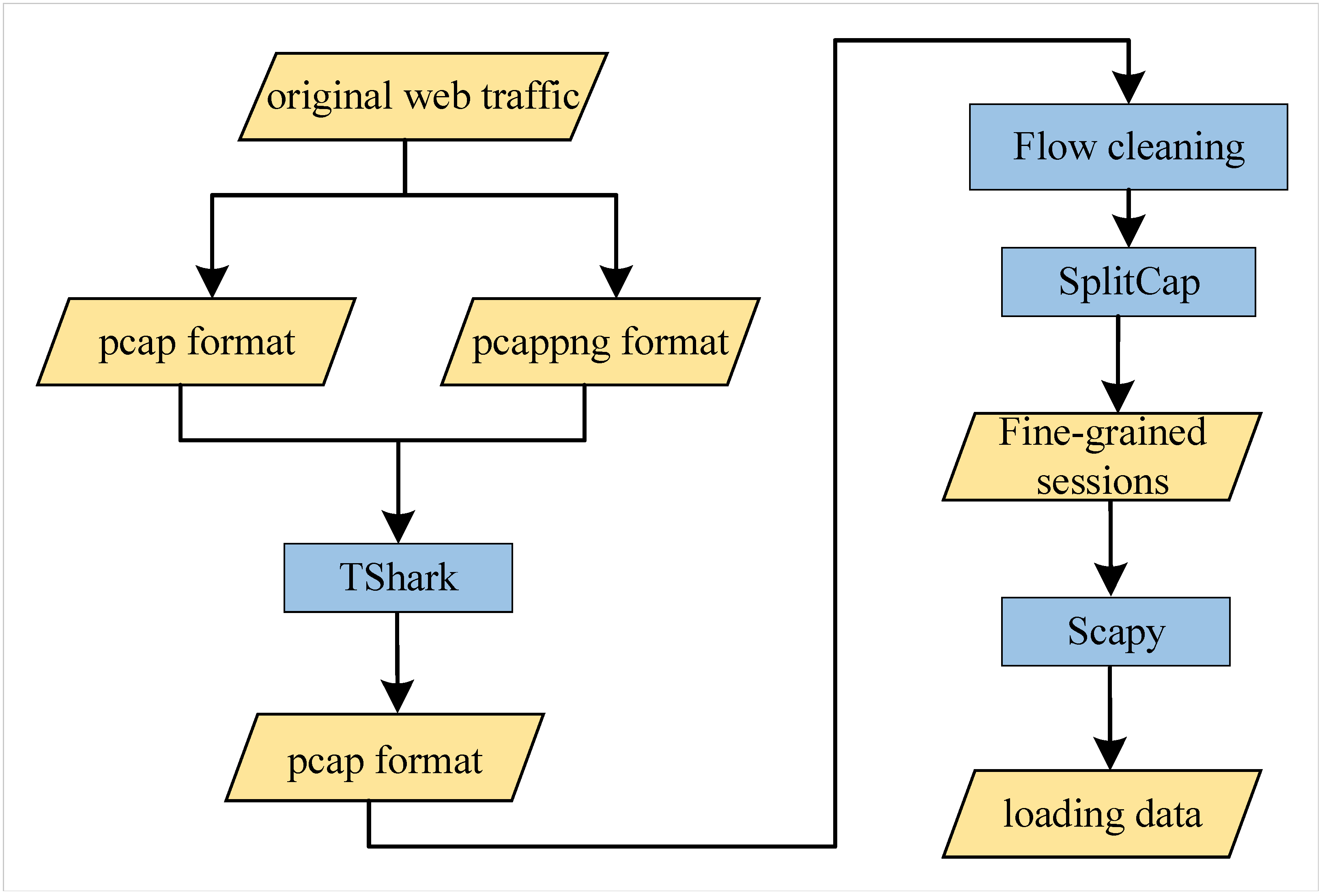
3.2. Data Preprocessing
| Algorithm 1: Data Preprocessing |
|
3.3. Algorithm for Generating Permutation Positive–Negative Sample Pairs (PNSPs)
3.3.1. Construction of Device Fingerprints Based on Grayscale Images
- (1)
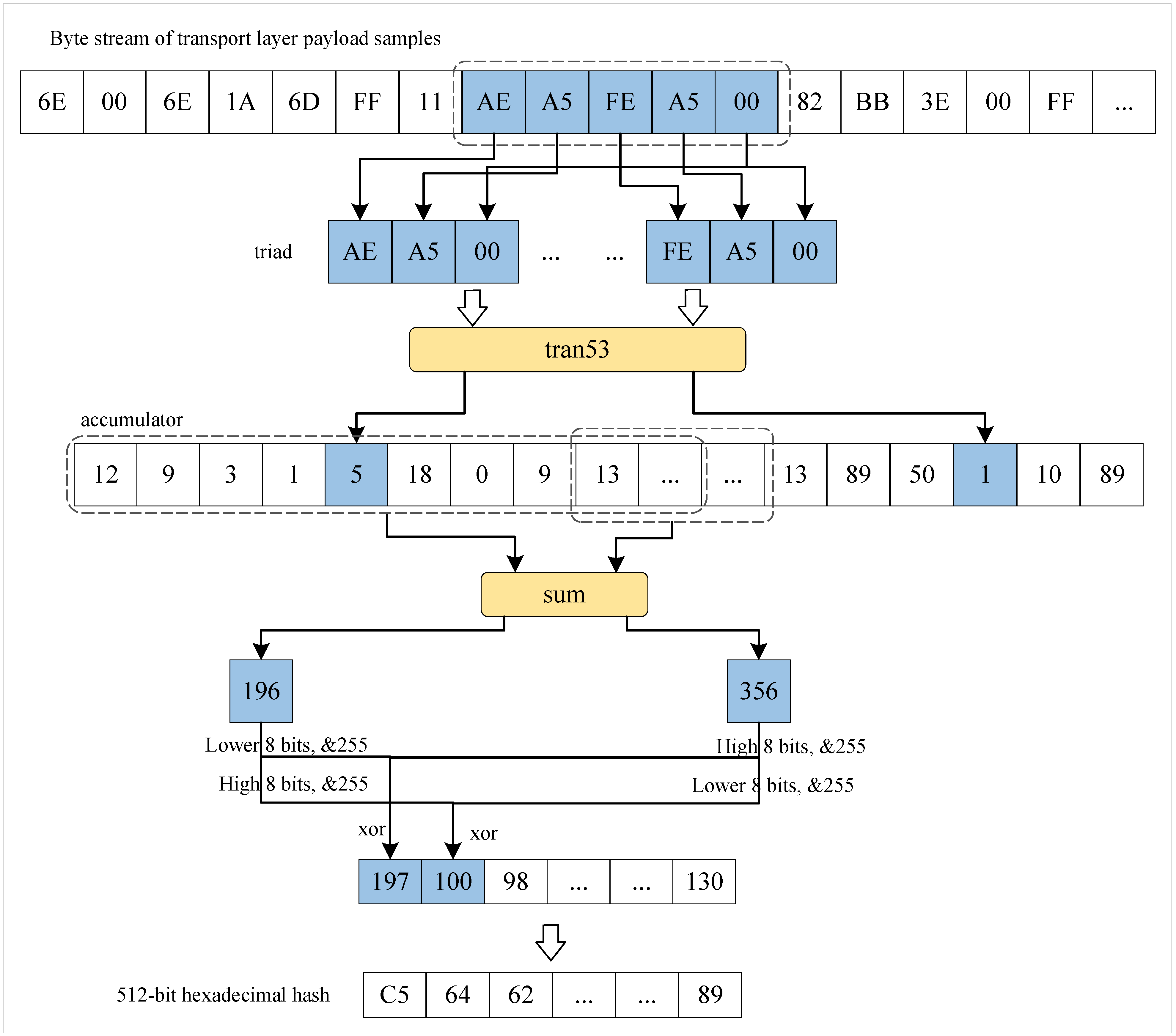
- A sliding window of size 5 with a step size of 1 is applied to the preprocessed payload data sample and slid to the right. Each window generates multiple triplets, denoted as , and each triplet is processed by the tran53 function to compute a value, denoted as .
- (2)
- A 512-length accumulator is defined. The value is used to indicate the index position of the accumulator. Each time an value is computed, the corresponding index position in the accumulator is incremented by 1. The sliding window shifts sequentially, and all accumulated values are stored in .
- (3)
- Two sliding windows, each with a size of 16 and a step size of 16, are defined to generate more accumulated values. The initial positions of the first and second windows are set to 0 and 8, respectively. The values in the first and second windows are summed, which are denoted as w and v, respectively. Since the length of is 512, each window must slide 32 times.
- (4)
- The accumulated values from the sliding window are processed via shift operations. First, the lower 8 bits of w are XORed with the upper 8 bits of to obtain , as shown in Equation (1). Subsequently, the upper 8 bits of w are XORed with the lower 8 bits of v to obtain , as shown in Equation (2). The final values are constrained to the range of 0–255 by applying a bitwise AND with 255, thus ensuring they are suitable for subsequent conversion into fixed-length hexadecimal hash values.
- (5)
- The sliding window continues to shift to the right across , thus ultimately producing a 512-bit hexadecimal locally sensitive hash value.
| Algorithm 2: Improved Nilsimsa Algorithm |
|
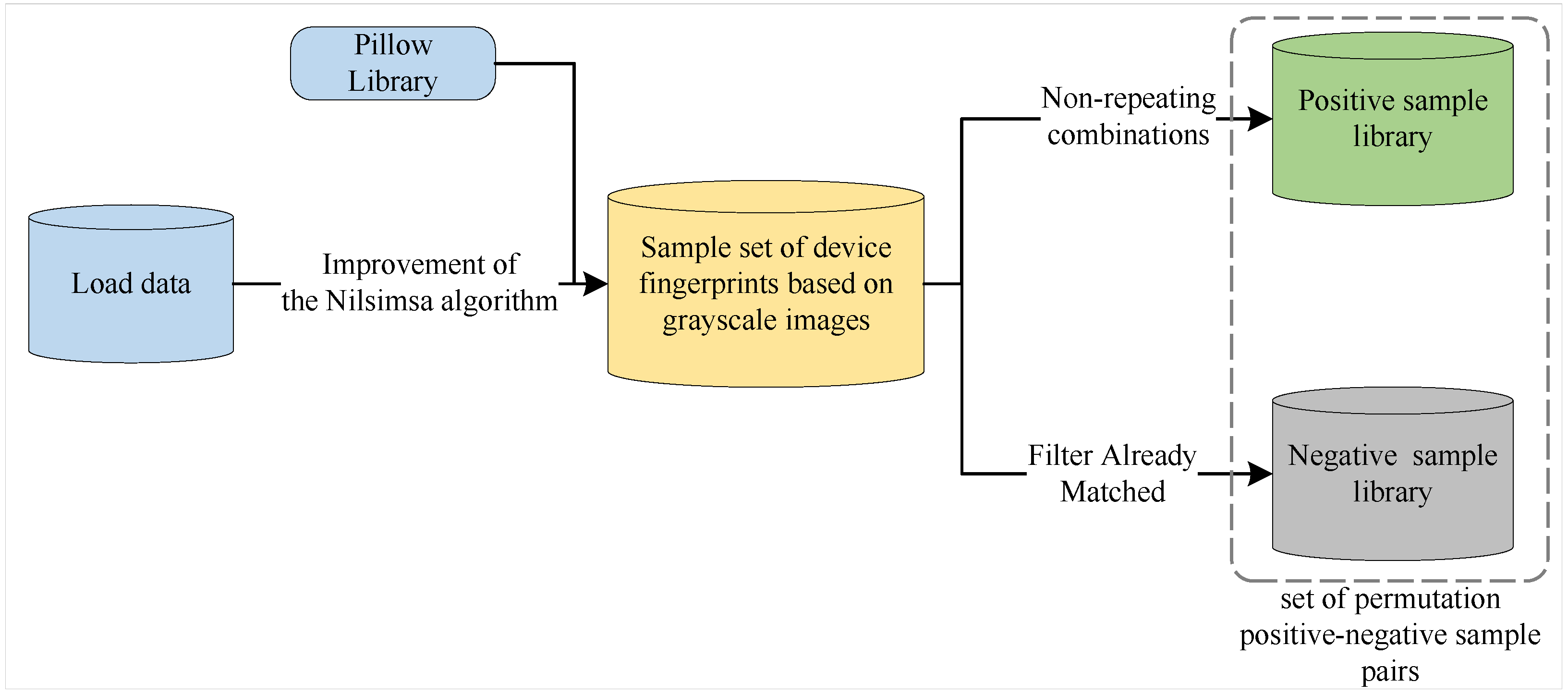
3.3.2. Generation of PNSPs
3.3.3. PNSP Algorithm
| Algorithm 3: PNSP Algorithm |
|
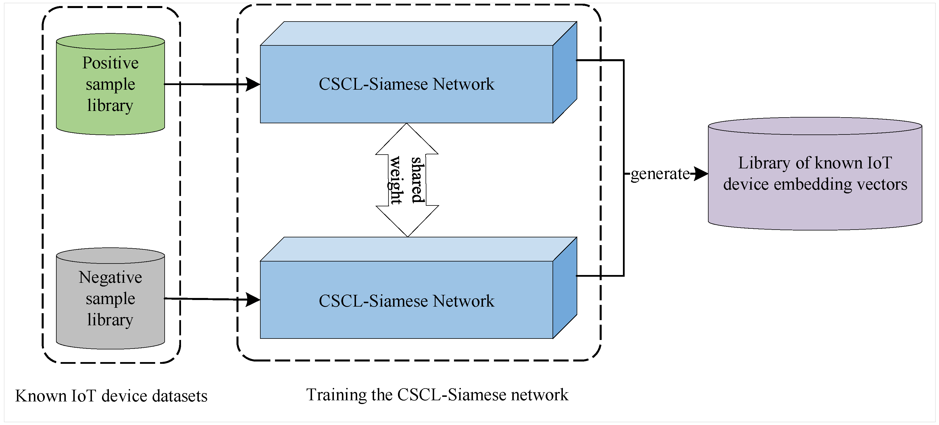
3.4. Embedding-Vector Database Generation Based on CSCL-Siamese Network: Embedding-Vector Database Construction (EVDC)-CSCL-Siamese Algorithm
3.4.1. PNSP Algorithm
3.4.2. CSCL Function
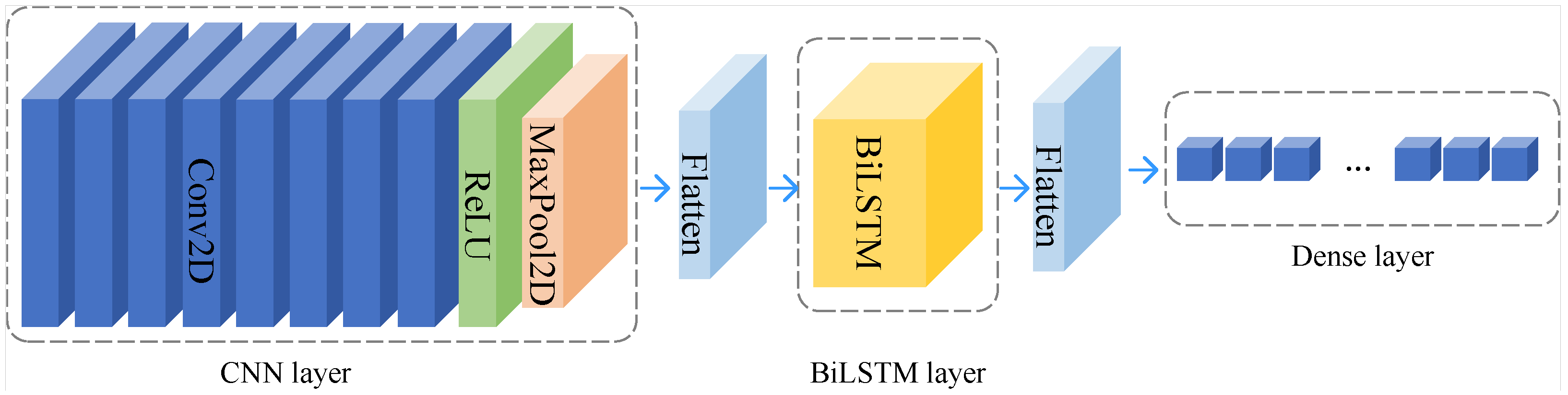
3.4.3. CSCL-Siamese Network
3.4.4. Embedding-Vector Database Generation Based on CSCL-Siamese Network
3.4.5. EVDC-CSCL-Siamese Algorithm
| Algorithm 4: EVDC-CSCL-Siamese Algorithm |
|
3.5. WVE-UDI: UDI Algorithm Based on WVE
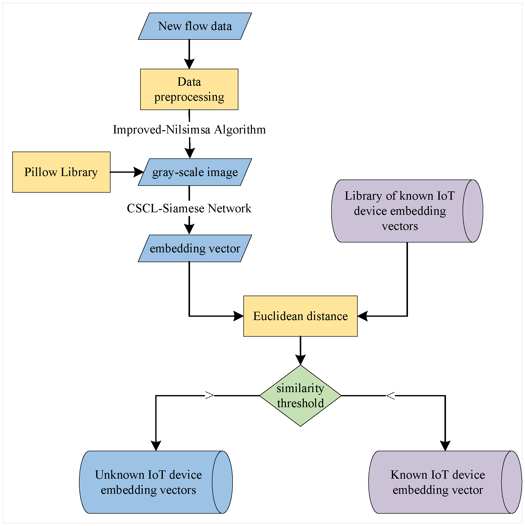
3.5.1. Filtering of Embedding Vectors for Unknown IoT Devices
3.5.2. WVE for UDI
3.5.3. WVE-UDI Algorithm
| Algorithm 5: WVE-UDI algorithm |
|
| Algorithm 6: CSCL-WVE-UDI approach |
|
4. Experimental Results and Analysis
4.1. Experimental Datasets
4.2. Evaluation Indicators
4.3. Experimental Environment and Experimental Parameter Settings
4.4. Experiments on the Efficiency of the CSCL-WVE-UDI Methodology
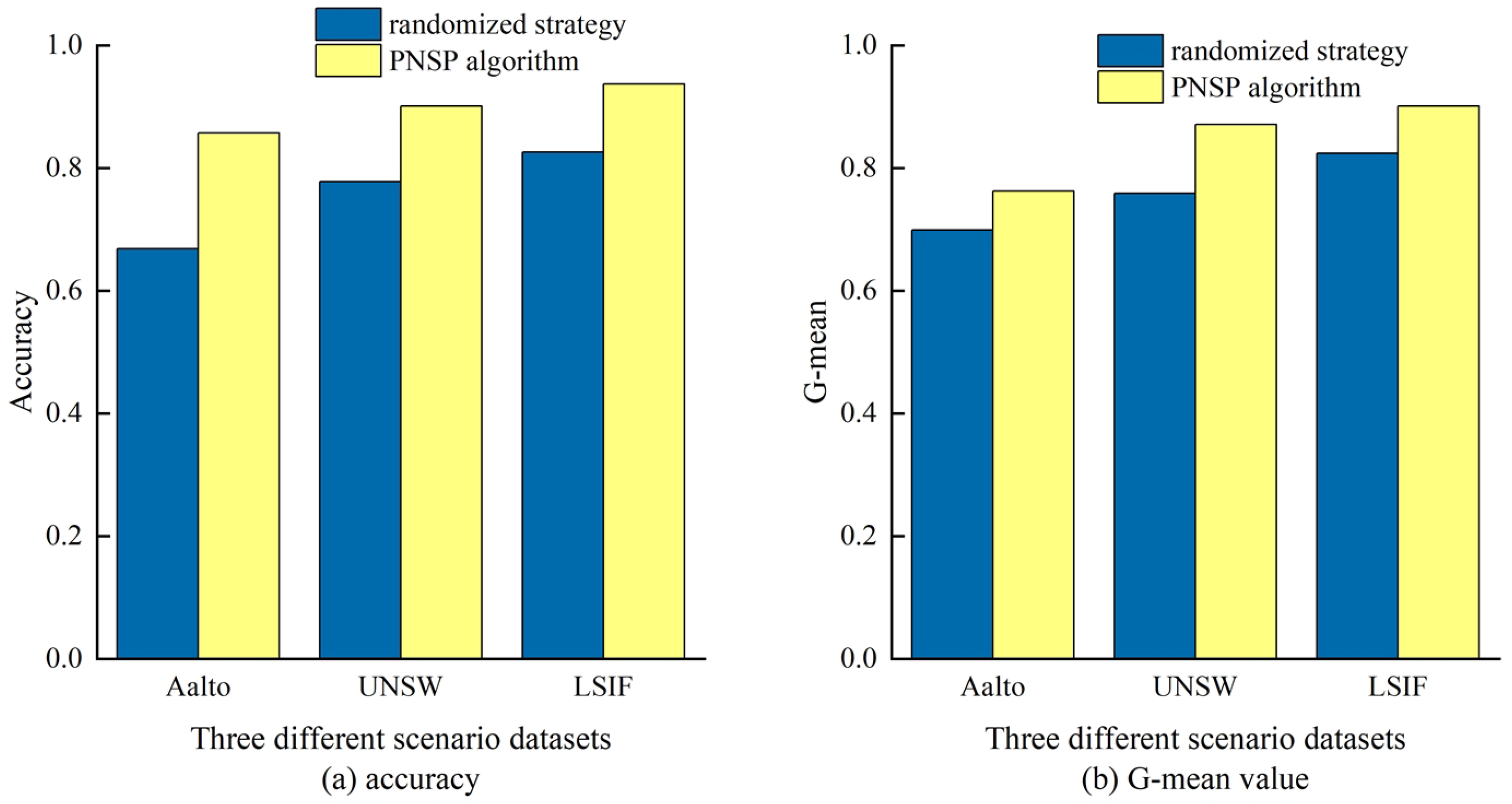
4.5. Comparative Experiments with PNSP Algorithm
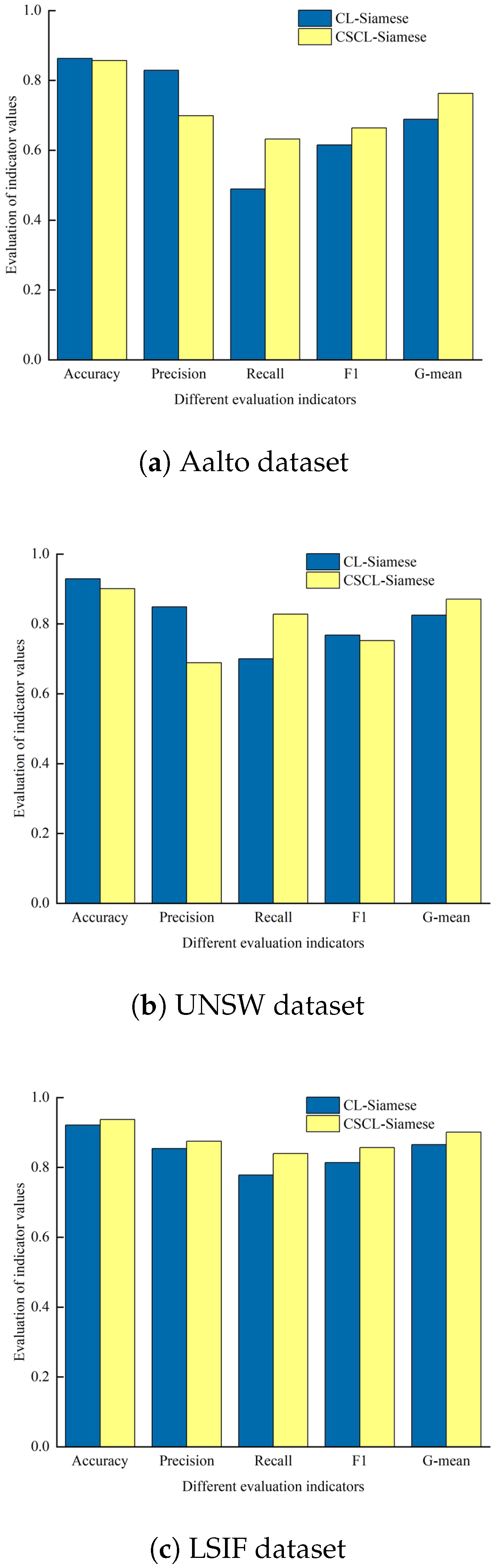
4.6. CSCL-Siamese Network Ablation Experiments
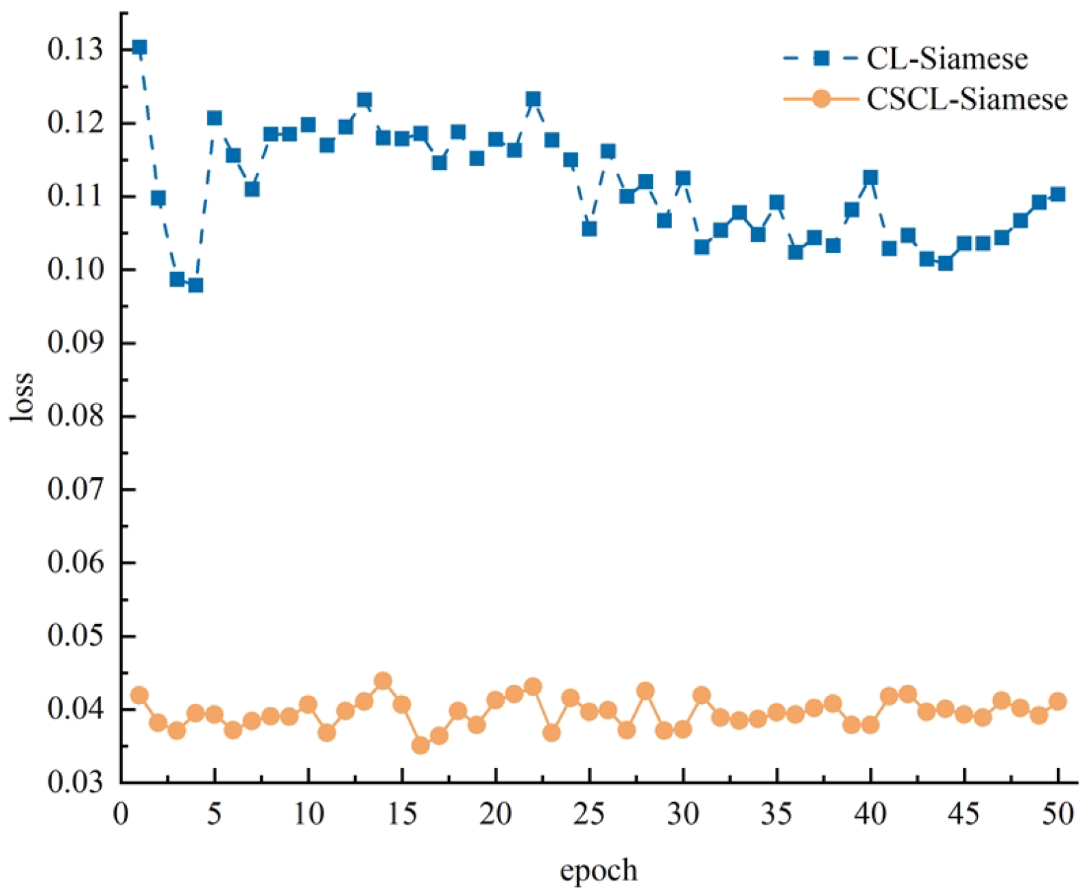
4.7. EVDC-CSCL-Siamese Algorithm Comparison Experiments
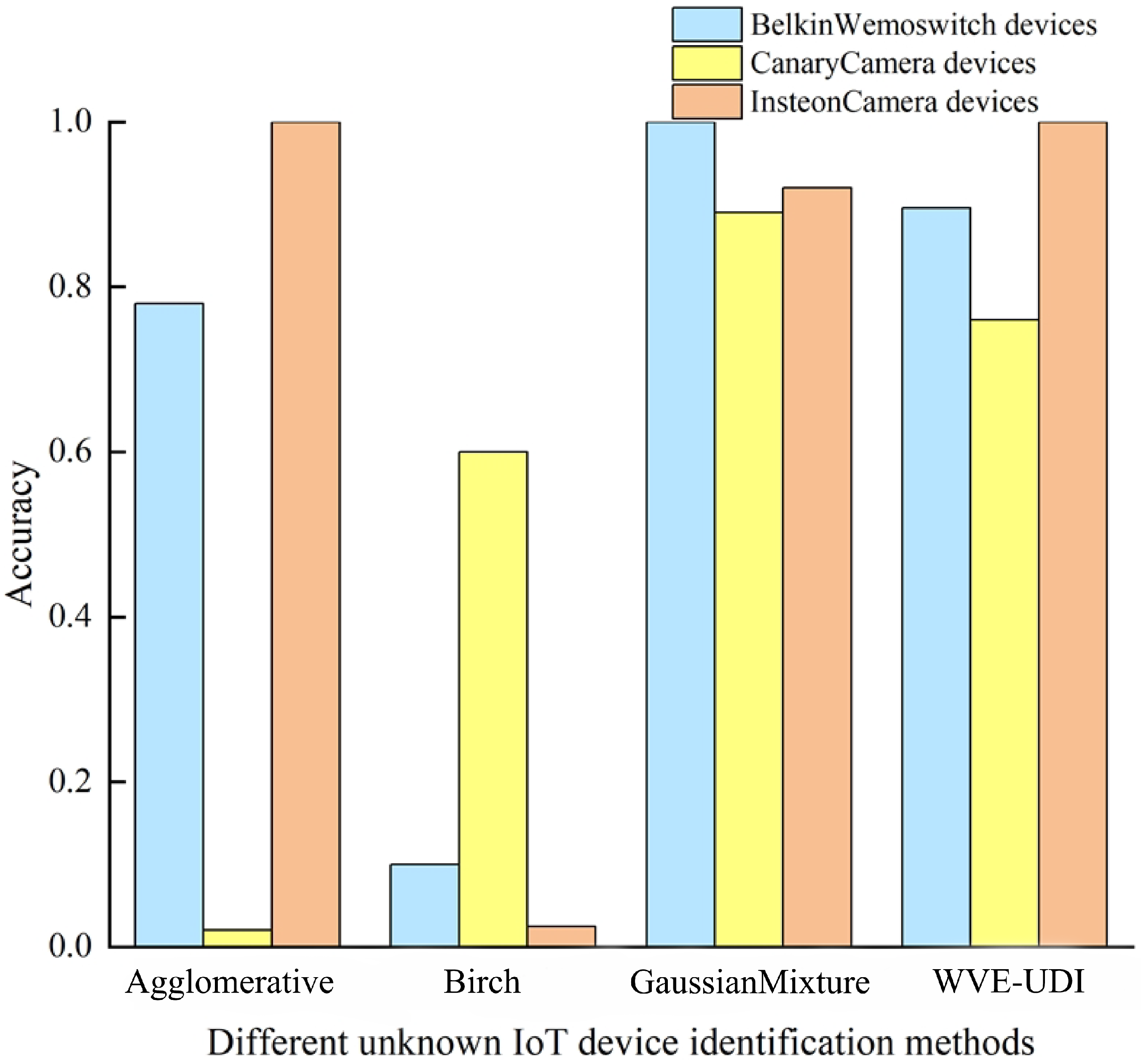
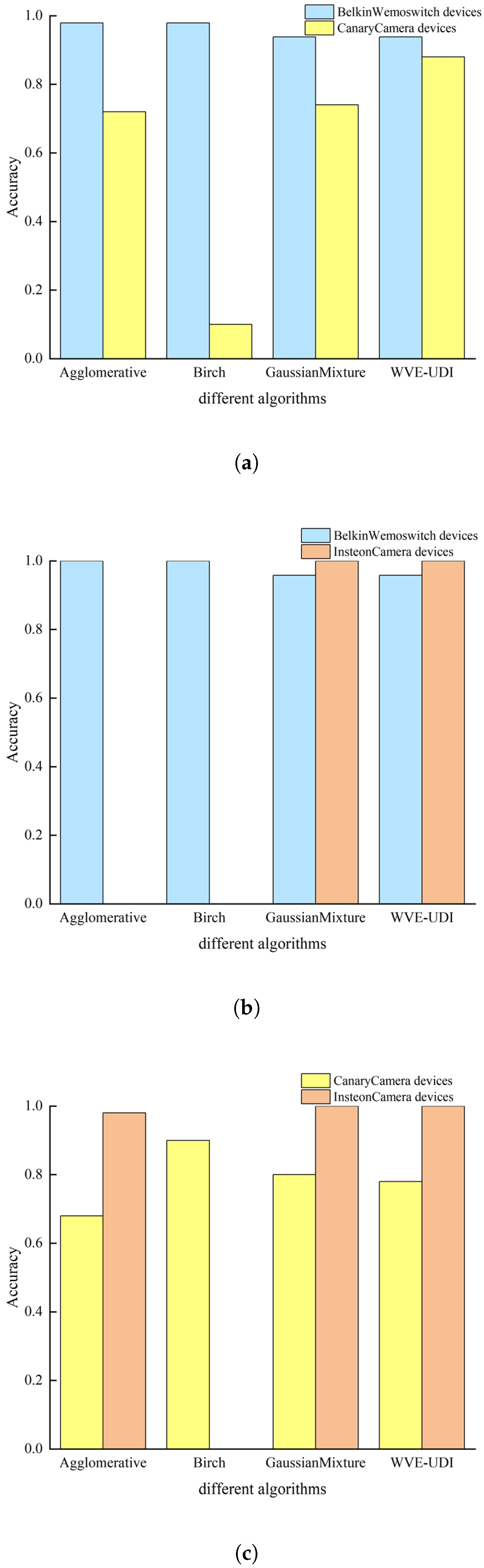
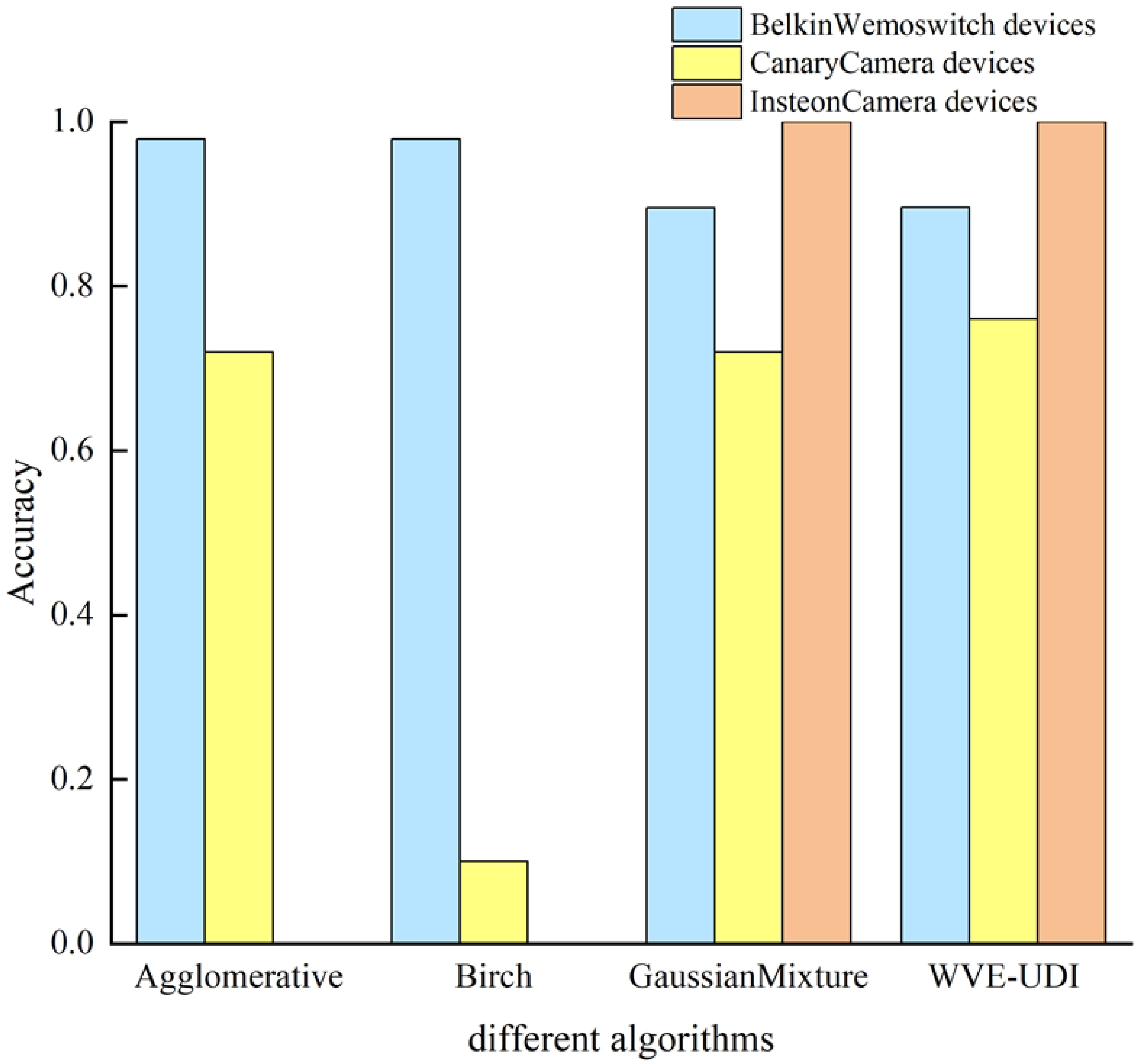
4.8. WVE-UDI Algorithm Ablation Experiments
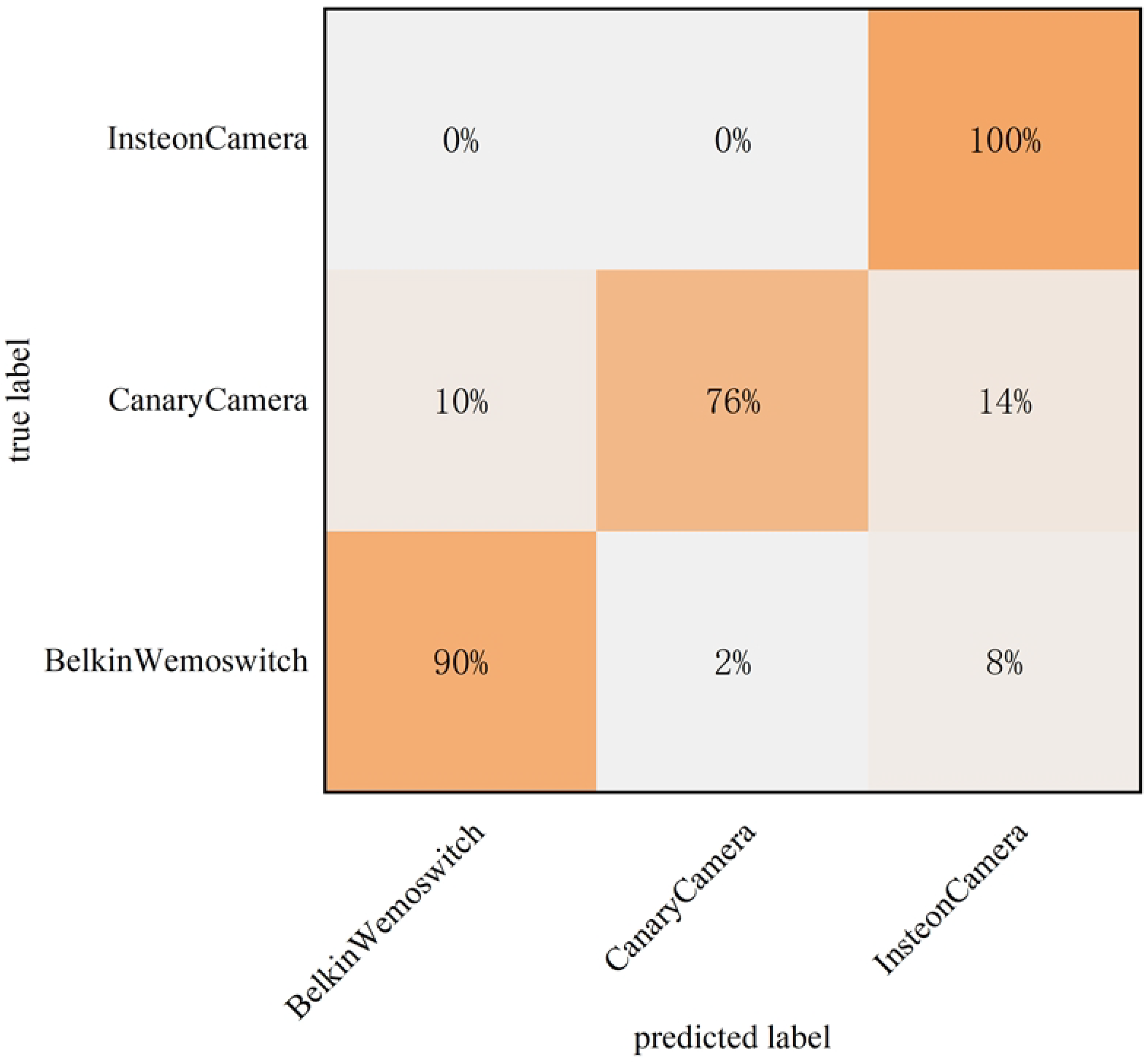
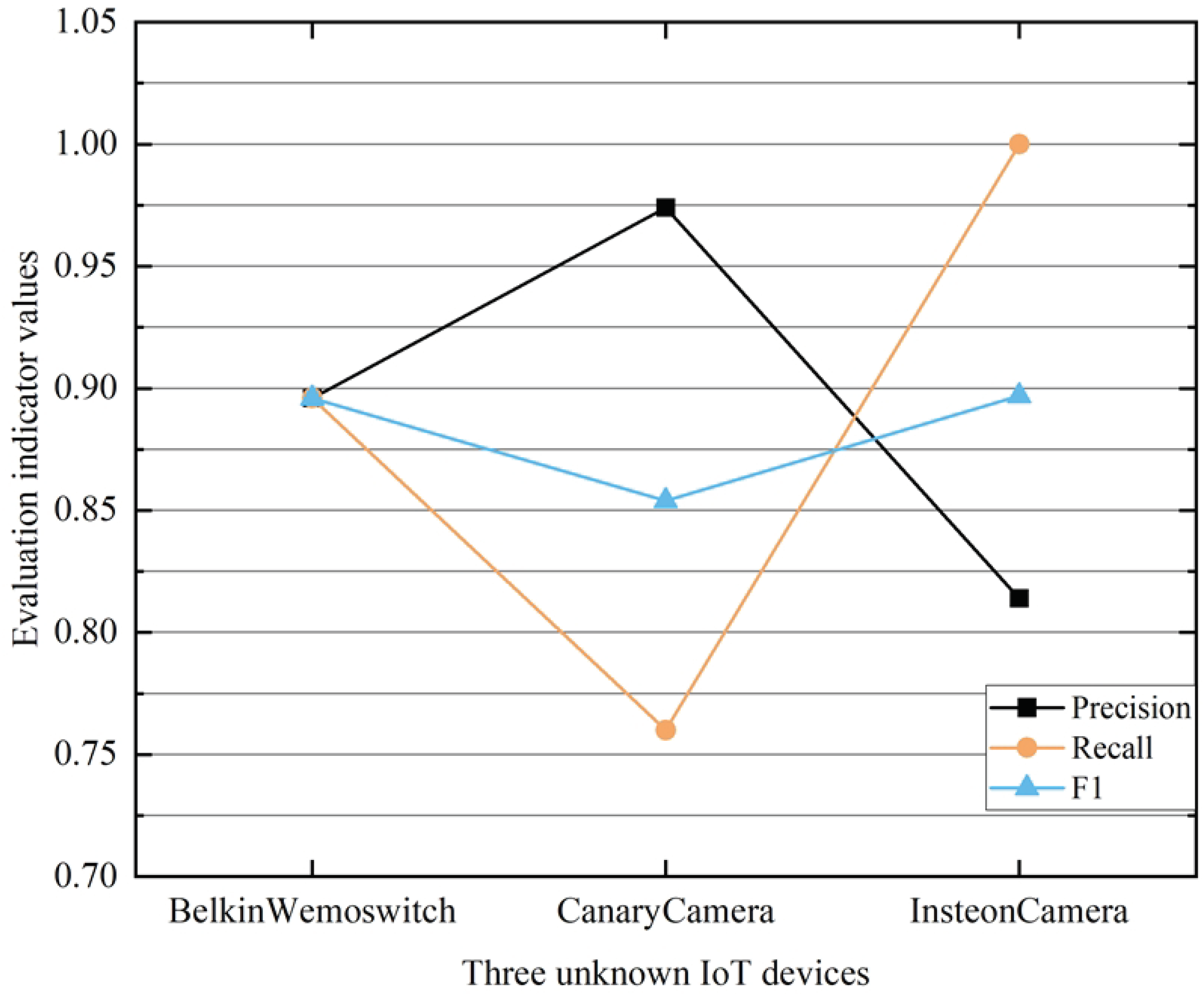
4.9. CSCL-WVE-UDI Method Validity Experiment
5. Conclusions
Author Contributions
Funding
Institutional Review Board Statement
Informed Consent Statement
Data Availability Statement
Conflicts of Interest
References
- Sasaki, Y. A survey on IoT big data analytic systems: Current and future. IEEE Internet Things J. 2021, 9, 1024–1036. [Google Scholar] [CrossRef]
- Luo, S.; He, R.; La, B. Research on Security Protection Technology for IoT Devices. Netw. Secur. Technol. Appl. 2023, 12, 24–26. [Google Scholar] [CrossRef]
- Aksoy, A.; Gunes, M.H. Automated iot device identification using network traffic. In Proceedings of the ICC 2019-2019 IEEE International Conference on Communications (ICC), Shanghai, China, 20–24 May 2019; pp. 1–7. [Google Scholar] [CrossRef]
- Zhang, S.; Xiao, K.; Yu, J.; Liu, X.; Wang, W. Accurate IoT Device Identification based on A Few Network Traffic. In Proceedings of the 2023 IEEE/ACM 31st International Symposium on Quality of Service, Orlando, FL, USA, 19–21 June 2023; pp. 1–10. [Google Scholar] [CrossRef]
- Trad, F.; Hussein, A.; Chehab, A. Using Siamese Neural Networks for Efficient and Accurate IoT Device Identification. In Proceedings of the 2022 Seventh International Conference on Fog and Mobile Edge Computing (FMEC), Paris, France, 12–15 December 2022; pp. 1–7. [Google Scholar] [CrossRef]
- Trad, F.; Hussein, A.; Chehab, A. Assessing the Effectiveness of Siamese Neural Networks to Mitigate Frequent Retraining in IoT Device Identification Models. In Proceedings of the 2023 International Conference on Platform Technology and Service (PlatCon), Busan, Republic of Korea, 16–18 August 2023; pp. 47–52. [Google Scholar] [CrossRef]
- Yin, S.; Zhang, W.; Feng, Y.; Xiang, Y.; Liu, Y. Automatic IoT device identification: A deep learning based approach using graphic traffic characteristics. Telecommun. Syst. 2023, 83, 101–114. [Google Scholar] [CrossRef]
- Bao, J.; Hamdaoui, B.; Wong, W.K. IoT Device Type Identification Using Hybrid Deep Learning Approach for Increased IoT Security. In Proceedings of the 2020 International Wireless Communications and Mobile Computing (IWCMC), Limassol, Cyprus, 15–19 June 2020; pp. 565–570. [Google Scholar] [CrossRef]
- Ross, J. Tshark, 2022. [EB/OL]. Available online: https://tshark.dev/export/ (accessed on 11 April 2024).
- Kotak, J.; Elovici, Y. IoT Device Identification Using Deep Learning. In 13th International Conference on Computational Intelligence in Security for Information Systems; Springer: Berlin/Heidelberg, Germany, 2020; pp. 76–86. [Google Scholar] [CrossRef]
- Potter, G.; Guillaume, V.; Pierre. Scapy. 2023. [EB/OL]. Available online: https://scapy.net/ (accessed on 11 April 2024).
- Damiani, E.; Vimercati, S.; Paraboschi, S.; Samarati, P. An Open Digest-based Technique for Spam Detection. Proceedings of ISCA 17th International Conference on Parallel and Distributed Computing Systems, San Francisco, CA, USA, 15–17 September 2004; pp. 559–564. [Google Scholar]
- Fuentealba, P.; Chamorro, E.; Santos, J.C. Chapter 5 Understanding and using the electron localization function. Theor. Asp. Chem. React. 2008, 19, 57–85. [Google Scholar] [CrossRef]
- Yin, F.; Li, Y.; Wang, Y.; Dai, J. IoT ETEI: End-to-End IoT Device Identification Method. In Proceedings of the 2021 IEEE Conference on Dependable and Secure Computing (DSC), Aizuwakamatsu, Japan, 30 January–2 February 2021; pp. 1–8. [Google Scholar] [CrossRef]
- Wang, F.; Liu, H. Understanding the behaviour of contrastive loss. In Proceedings of the IEEE/CVF Conference on Computer Vision and Pattern Recognition, Nashville, TN, USA, 20–25 June 2021; pp. 2495–2504. [Google Scholar]
- Hu, J.; Wang, J. Prediction of liquefaction of gravelly soils based on a cost-sensitive Bayesian network combined with rough set weighting. Gondwana Res. 2024, 131, 57–68. [Google Scholar] [CrossRef]
- Majhi, M.; Pal, A.K.; Islam, S.K.H.; Khurram Khan, M. Secure content-based image retrieval using modified Euclidean distance for encrypted features. Trans. Emerg. Telecommun. Technol. 2021, 32, e4013. [Google Scholar] [CrossRef]
- Bamhdi, A.M.; Abrar, I.; Masoodi, F. An ensemble based approach for effective intrusion detection using majority voting. Telkomnika Telecommun. Comput. Electron. Control. 2021, 19, 664–671. [Google Scholar] [CrossRef]
- Tokuda, E.K.; Comin, C.H.; Costa, L.F. Revisiting agglomerative clustering. Phys. A Stat. Mech. Appl. 2022, 585, 126433. [Google Scholar] [CrossRef]
- Yin, S.; Li, H.; Liu, D.; Karim, S. Active contour modal based on density-oriented BIRCH clustering method for medical image segmentation. Multimed. Tools Appl. 2020, 79, 31049–31068. [Google Scholar] [CrossRef]
- Shieh, C.S.; Lin, W.W.; Nguyen, T.T.; Chen, C.H.; Horng, M.F.; Miu, D. Detection of unknown ddos attacks with deep learning and gaussian mixture model. Appl. Sci. 2021, 11, 5213. [Google Scholar] [CrossRef]
- ACRIS. IoT Devices Setup Captures, 2017. [EB/OL]. Available online: https://research.aalto.fi/en/datasets/iot-devices-captures (accessed on 11 April 2024).
- Sivanathan, A.; Gharakheili, H.H.; Loi, F.; Radford, A.; Wijenayake, C.; Vishwanath, A.; Sivaraman, V. Classifying IoT devices in smart environments using network traffic characteristics. IEEE Trans. Mob. Comput. 2019, 18, 1745–1759. [Google Scholar] [CrossRef]
- Charyyev, B.; Gunes, M.H. IoT Traffic Flow Identification using Locality Sensitive Hashes. In Proceedings of the ICC 2020–2020 IEEE International Conference on Communications, Dublin, Ireland, 7–11 June 2020; pp. 1–6. [Google Scholar] [CrossRef]
- Thom, J.; Thom, N.; Sengupta, S.; Hand, E. Smart Recon: Network Traffic Fingerprinting for IoT Device Identification. In Proceedings of the 2022 IEEE 12th Annual Computing and Communication Workshop and Conference (CCWC), Las Vegas, NV, USA, 26–29 January 2022; pp. 72–79. [Google Scholar] [CrossRef]
- Bruhadeshwar, B.; Maalvika, B.; Jordan, P.; Shirazi, H.; Ray, I.; Ray, I. Behavioral Fingerprinting of IoT Devices; Association for Computing Machinery—ACM: New York, NY, USA, 2018; pp. 41–50. [Google Scholar] [CrossRef]
- Kostas, K.; Just, M.; Lones, M.A. IoTDevID: A Behavior-Based Device Identification Method for the IoT. IEEE Internet Things J. 2022, 9, 23741–23749. [Google Scholar] [CrossRef]


| Symbol | Definition | Symbol | Definition |
|---|---|---|---|
| Raw traffic sample of the i-th IoT device | Preprocessed payload data of the i-th device | ||
| 512-bit hexadecimal hash value from improved Nilsimsa | Grayscale image fingerprint of the j-th sample from device i | ||
| Set of positive sample pairs | Set of negative sample pairs | ||
| W | Network weight parameters | 256D embedding vectors of samples a and b | |
| Label for sample pair (1=same class, 0=different class) | Weighting factor for positive pairs: | ||
| Weighting factor for negative pairs: | Manhattan distance: | ||
| m | Minimum acceptable distance threshold for negative pairs | L | CSCL loss function |
| Embedded vector database for known devices | Embedded vectors of new traffic data | ||
| Minimum Euclidean distance | Similarity threshold for filtering unknown devices | ||
| Clustering results (Agglomerative/BIRCH/GaussianMixture) | Weights for clustering algorithms (0.2/0.2/0.6) | ||
| Cluster label of sample i by Agglomerative | Final identification results of unknown devices | ||
| True positive/negative counts | False positive/negative counts | ||
| G−mean | Geometric mean of TPR and TNR | Number of positive/negative sample pairs |
| Dataset Name | Number of Positive Samples | Number of Negative Pair Samples |
|---|---|---|
| Aalto | 8008 | 25,968 |
| UNSW | 11,000 | 46,000 |
| LSIF | 8800 | 28,800 |
| Positive Class | Negative Class | |
|---|---|---|
| Predicted | TP (Positive class predicted to be positive) | FP (Negative class predicted to be positive) |
| Unpredicted | FN (Positive class predicted to be negative) | TN (Negative class predicted to be negative) |
| Software and Hardware Type | Value |
|---|---|
| System | Windows10 |
| CPU | AMD Ryzen 7 5800H |
| GPU | NVIDIA GeForce RTX 3060 |
| Programming language | Python3.8 |
| Deep Learning Framework | Keras2.4.3 |
| Parameter Name | Parameter Value |
|---|---|
| Optimizer | Adam |
| Learning rate | 0.001 |
| Batch size | 64 |
| Epochs | 50 |
| Factor | 0.1 |
| Patience | 3 |
| Min learning rate | 0.0001 |
| Unknown IoT Devices | Belkin Wemo Switch | Canary Camera | Insteon Camera | |
|---|---|---|---|---|
| Algorithms | ||||
| Agglomerative algorithm | 100% | 90% | 100% | |
| Birch algorithm | 100% | 90% | 100% | |
| GaussianMixture algorithm | 100% | 100% | 100% | |
| WVE-UDI algorithm | 100% | 90% | 100% | |
Disclaimer/Publisher’s Note: The statements, opinions and data contained in all publications are solely those of the individual author(s) and contributor(s) and not of MDPI and/or the editor(s). MDPI and/or the editor(s) disclaim responsibility for any injury to people or property resulting from any ideas, methods, instructions or products referred to in the content. |
© 2025 by the authors. Licensee MDPI, Basel, Switzerland. This article is an open access article distributed under the terms and conditions of the Creative Commons Attribution (CC BY) license (https://creativecommons.org/licenses/by/4.0/).
Share and Cite
Qian, J.; Zheng, W.; Lu, X.; Li, Z. Unknown IoT Device Identification Models and Algorithms Based on CSCL-Siamese Networks and Weighted-Voting Clustering Ensemble. Appl. Sci. 2025, 15, 5274. https://doi.org/10.3390/app15105274
Qian J, Zheng W, Lu X, Li Z. Unknown IoT Device Identification Models and Algorithms Based on CSCL-Siamese Networks and Weighted-Voting Clustering Ensemble. Applied Sciences. 2025; 15(10):5274. https://doi.org/10.3390/app15105274
Chicago/Turabian StyleQian, Junhao, Wenyu Zheng, Xulin Lu, and Zhihua Li. 2025. "Unknown IoT Device Identification Models and Algorithms Based on CSCL-Siamese Networks and Weighted-Voting Clustering Ensemble" Applied Sciences 15, no. 10: 5274. https://doi.org/10.3390/app15105274
APA StyleQian, J., Zheng, W., Lu, X., & Li, Z. (2025). Unknown IoT Device Identification Models and Algorithms Based on CSCL-Siamese Networks and Weighted-Voting Clustering Ensemble. Applied Sciences, 15(10), 5274. https://doi.org/10.3390/app15105274