Article

Interpretability Study of Gradient Information in Individual Travel Prediction

1
Institute of Physics, Henan Academy of Sciences, Zhengzhou 450046, China
2
School of Mechanical and Electrical Engineering, Henan University of Science and Technology, Luoyang 471003, China
*
Author to whom correspondence should be addressed.
Appl. Sci. 2025, 15(10), 5269; https://doi.org/10.3390/app15105269
Submission received: 26 February 2025 / Revised: 23 April 2025 / Accepted: 30 April 2025 / Published: 9 May 2025
(This article belongs to the Section Computing and Artificial Intelligence)

Abstract

With the development of intelligent transportation systems (ITS), individual travel prediction has become a key technology for optimizing urban transportation. However, deep learning models are limited in decision-sensitive scenarios due to their lack of interpretability. To address the shortcomings of existing XAI methods in analyzing the dynamic features of historical travel sequences, this paper introduces an alternative interpretability method based on gradient information, overcoming the interpretability bottleneck of travel prediction models. This method calculates the gradient information of input features relative to the prediction result, breaking through the limitations of traditional interpreters that only analyze static features. It can trace the contribution weights of key time points in historical travel sequences while maintaining low computational cost. The experimental results show that features with higher gradients significantly affect predictions—masking the maximum-gradient feature reduces accuracy by approximately 30%. Descending-order masking strategies exhibit the strongest impact, highlighting nonlinear interactions among features. Contribution maps visualize how gradients capture regular patterns and anomalies. The method proposed in this paper provides a valuable tool for understanding the underlying principles of travel prediction models, bridging the gap in existing methods for temporal sequence analysis.

1. Introduction

As the global urbanization process accelerates, the spatiotemporal complexity of urban transportation systems grows exponentially, driving intelligent transportation systems (ITS) to become a strategic technology for optimizing urban operational efficiency [1]. Individual travel prediction, as the core technical support for ITS, provides decision-making basis for dynamic traffic scheduling and resource optimization by mining the spatiotemporal association features in passenger behavior patterns [2,3,4]. However, traditional machine learning methods face limitations in representing high-dimensional, nonlinear traffic data. While deep learning models can capture complex patterns, their inherent opacity makes the prediction mechanisms difficult to interpret, which severely restricts their application in decision-sensitive scenarios [5].
In recent years, explainable artificial intelligence (XAI) methods [6] have made significant progress across various fields, but they face unique challenges in the context of travel behavior prediction. Current research largely relies on mainstream interpreters such as SHAP [7] and LIME [8], which perform excellently in static feature attribution analysis, but have significant limitations when it comes to explaining temporal features. Existing methods can only explain the impact of static features and fail to reveal the dynamic association mechanisms of historical travel sequences, as shown in Figure 1. For example, in epidemic transmission chain tracing, decision-makers not only need to predict the future travel locations of individuals but also need to identify the contribution weights of key historical nodes (e.g., specific dates and locations) to the current prediction. This is crucial for formulating effective control strategies [9]. Existing XAI methods, due to their lack of capability to deconstruct temporal associations, lead to explanatory results that are insufficient to meet decision-making needs [10].
To address the interpretability bottleneck in individual travel prediction, this study introduces for the first time a gradient-based saliency method into the travel prediction field, filling the gap in existing XAI methods in analyzing the dynamic features of historical travel sequences. This method constructs a spatiotemporal feature contribution map by calculating the gradient response of input features to the prediction result. Its technical advantages are reflected in three dimensions: first, it breaks through the limitation of traditional interpreters that only analyze static features, allowing the tracking of contribution weights of key time points in the historical travel sequence; second, by generating spatiotemporal heatmaps with the same dimensions as the original data, it converts abstract features like departure time and station numbers into visual decision-making references; third, compared to the exponential computational demands of mainstream interpreters [11], this method has linear complexity with respect to model parameters, offering significant computational advantages in long-sequence analysis. This choice of technical path does not question the theoretical value of existing XAI methods but instead provides new perspectives and methods for expanding interpretability in the travel prediction domain through domain transfer.
The study conducts experiments based on real travel data from a city’s subway system, and the results show that gradient information can effectively quantify feature contribution, with the most significant gradient features accounting for over 30% of the impact on prediction performance. This finding not only provides a new method for the interpretability of individual travel prediction models but also lays a theoretical foundation for trustworthy decision-making in intelligent transportation systems. Here, we would like to emphasize that our choice to explore the gradient-based saliency method instead of directly applying advanced interpreters is not aimed at comparing the superiority of different interpretability strategies. On the contrary, the motivation behind our research is to explore and understand the role and value of gradient information in revealing the decision-making process of travel prediction models, which may bring new insights to this field.

2. Related Work

The current research on the interpretability of travel prediction models mainly focuses on two technical routes: the transparent model interpretability framework and the post hoc interpretability framework, as shown in Figure 2.

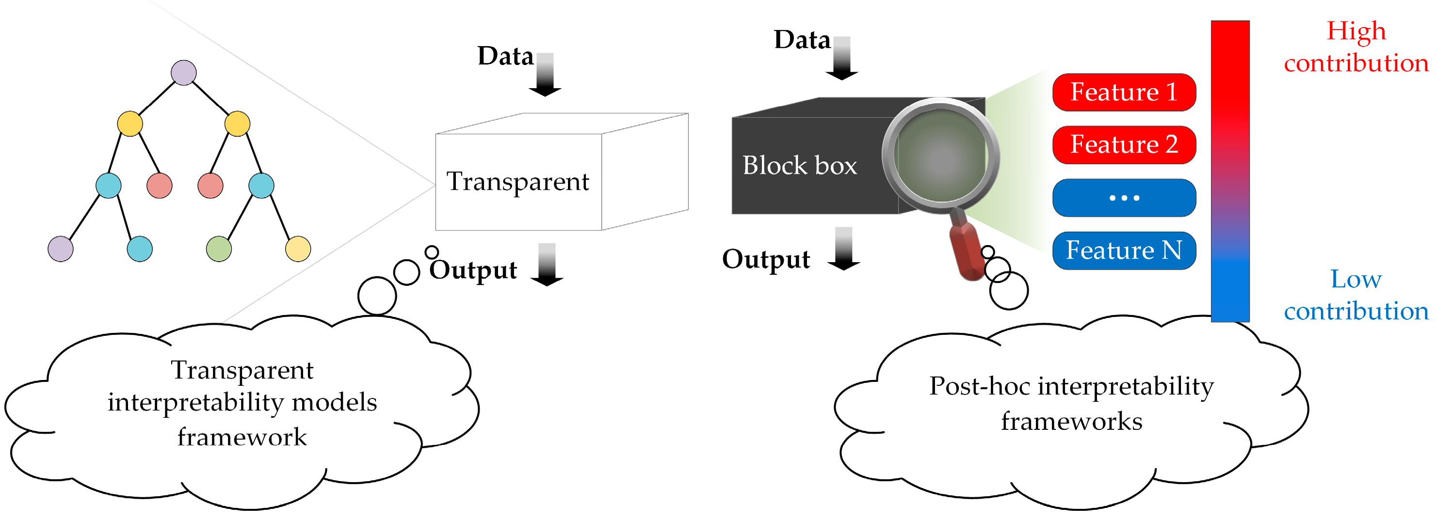
2.1. Transparent Interpretability Models Framework

The core advantage of the transparent model interpretability framework lies in the mathematical interpretability that the model itself can provide [12]. Through structured decision logic and explicit feature interaction relationships, researchers can directly trace the transformation process from input to output. In the field of individual travel analysis, decision tree models [13] achieve this goal through a recursive feature space partitioning mechanism: each internal node in the tree structure selects the splitting feature based on the information gain maximization criterion, which is specifically quantified as follows:
I G ( D , f ) = H ( D ) v = 1 V | D v | D H ( D v )
where H ( D ) = p k log p k represents the entropy of the parent node, and D v is the subset of data where feature f takes value v . The prediction process of the decision tree can be formalized as an explicit rule combination:
f ( x ) = i = 1 K v i · I ( x R i )
where x represents the input features, R i represents the feature space region corresponding to the i t h leaf node, v i represents the predicted value of the i t h leaf node, and I is the indicator function. When x R i , it takes the value of 1, otherwise, it is 0, and K represents the total number of leaf nodes. This formula implies that, for an input x , the prediction result is based on the feature space region R i it belongs to, and the corresponding leaf node prediction value v i is taken as the output, allowing users to clearly identify the decision-making process based on the features in the model [14]. The interpretability of decision trees can also be transferred to more complex models through rule extraction techniques [15], thus constructing an interpretable travel behavior prediction framework [16].
Compared with the visualization of static rules by decision trees, Markov models provide interpretability for temporal behavior modeling through dynamic probability transfer mechanisms [17]. The core assumption is the memoryless property of state transitions, meaning that the future state of the system depends only on the current state, not on the history. If the system is in state s i at time s t , the probability of transitioning to state s j at the next time step depends only on the current state s i , which can be represented by the transition probability matrix:
A = [ P ( s t + 1 = s j | s t = s i ) ]
This property gives Markov models unique value in dynamic scenarios such as short-term traffic flow forecasting and user movement trajectory modeling [18]. Furthermore, the hidden Markov model (HMM) infers the transition and generation processes of hidden states from observed data, making it more suitable for handling complex temporal problems with underlying patterns. For example, by analyzing historical GPS trajectory data to construct a transition probability matrix, it can predict an individual’s next visited location [19,20]. Transparent interpretability models, through simplified logic and clear decision-making processes, provide users and decision-makers with easily understandable predictions. However, this approach is limited by the transparent structure of the model, making it difficult to extend to deep learning models.

2.2. Post Hoc Interpretability Framework

To compensate for the limitations of the transparent model interpretability framework, the post hoc interpretability framework adds an additional model architecture on top of the original model to specifically explain the decision-making process of the original model [21].
As a representative of this framework, SHapley Additive exPlanations (SHAP) [7] provides a new perspective for explaining predictions from any machine learning model with its unique capabilities. SHAP is a game theory-based model explanation method that can effectively reveal relationships between travel features [22,23,24,25,26]. The core idea is to calculate the Shapley value of feature contributions, treating machine learning predictions as the outcome of a cooperative game between “feature players”. Each feature’s contribution φ i is calculated by the weighted average of its marginal contributions as follows:
φ i = S F \ { i } | S | ! ( | F | | S | 1 ) ! | F | ! ( v ( S { i } ) v ( S ) )
where, v ( S { i } ) v ( S ) represents the marginal contribution of i to S ; S F \ { i } indicates the need to sum up all possible alliances; | S | ! ( | F | | S | 1 ) ! | F | ! represents the weight of the alliance. SHAP can be defined, for an input sample x , its prediction f ( x ) can be expressed as the sum of a baseline value φ 0 and the contributions of each feature φ i :
f ( x ) = φ 0 + i = 1 M φ i
To obtain the precise Shapley values for all features, it means generating all possible feature coalitions for the input, which grows exponentially with the number of features in the model. To reduce computational complexity, KernelSHAP [27] approximates the local behavior of complex models with a linear model of feature importance, defining a kernel-weighted squared loss function as follows:
L = z [ f ( h x ( z ) ) g ( z ) ] 2 π x ( z )
where z is the feature mask vector, h x is the feature mapping function, g is the linear explanation model, and π x is the sample weight kernel function. Although KernelSHAP has been widely adopted, its perturbation only affects the instance being explained and ignores the model’s hidden states, meaning that in the field of travel prediction dominated by RNNs, there is a mismatch between the data KernelSHAP assigns importance to and the data the model actually relies on.
Further, TimeSHAP [28] builds on KernelSHAP and extends it to the sequence domain. TimeSHAP is implemented through KernelSHAP’s sampling framework, but modifies the feature mask generation logic z expanding it from a single-time feature mask to a time-slice level mask, thus solving the interpretability problem in time series prediction. The method uses a linear explainer g to approximate the model’s local behavior as follows:
f ( h X ( z ) ) g ( z ) = w 0 + i = 1 m w i z i
TimeSHAP approximates the local behavior of complex explainers through the calculation of the loss function, allowing the explainer to simultaneously capture feature interactions across time steps. TimeSHAP can explain which features in history have the largest impact on the current prediction [29]. A prominent issue with TimeSHAP is that the computational time grows exponentially with the length of the observation sequence [30], making the computational cost prohibitive when handling longer sequences.
Unlike the global explanations provided by SHAP, Local Interpretable Model-agnostic Explanations (LIME) [8] is a local explanation method that simplifies the decision boundary of a complex model into a linear hyperplane around the target point using local linear approximation. For a target sample x , LIME generates a set of perturbed samples { z i } in its neighborhood. These perturbed samples are passed through the black-box model f , yielding corresponding predictions f ( z i ) , forming a new dataset { ( z i , f ( z i ) ) } . Based on the perturbed dataset, LIME trains an interpretable linear model by minimizing the weighted loss function as follows:
arg min g G i π x ( z i ) [ f ( z i ) g ( z i ) ] 2 + Ω ( g )
where π x ( z i ) is sample weight function that responds to the similarity between the perturbed sample z i and the original sample x , Ω ( g ) is regularization, and G is a set of simple models. LIME was originally designed to explain a single prediction, but through sensitivity analysis of perturbations, it can identify the most influential features for a particular prediction, indirectly revealing the key factors on which the decision depends [31,32,33,34]. However, the quality of LIME’s explanations depends on the reasonable choice of perturbation range and the proper definition of sample weights, and it cannot reveal the temporal dependencies in travel prediction tasks when revealing relationships between different features.
Compared to the methods mentioned above, the gradient-based saliency method introduced in this paper not only explains the static feature distribution on which the model’s overall decision depends, but also identifies the key historical input points for specific prediction samples. Unlike TimeSHAP, which requires exhaustive evaluation of the marginal contributions of all feature coalitions, this method only requires backward propagation to obtain the feature importance scores for the sequence, with computational complexity linearly related to the number of model parameters. To quantify this computational advantage, we selected 1000 samples and compared the time consumption for explaining each sample. The experimental results show that the average explanation time for TimeSHAP is 38.18 s, while the proposed method only takes 3.15 s, reducing the time cost by approximately 91.7%, improving computational efficiency by an order of magnitude, and providing the possibility for real-time prediction explanations in the future. Table 1 shows a comparison between the proposed method and the current mainstream interpretability solutions in the field of travel prediction, emphasizing its progress in computational efficiency and spatiotemporal dependency analysis.

3. Methods

This chapter will systematically explore how to enhance the interpretability of deep learning models in individual travel prediction. First, we will introduce the concepts of individual travel prediction and interpretability. Then, through analogy with image recognition tasks, we will reveal the similarities between these tasks in terms of pattern recognition and feature contribution. This analogy will provide the theoretical foundation for introducing saliency methods.

3.1. Individual Travel Prediction and the Concept of Interpretability

Individual travel prediction is based on the regularity of travel behavior, meaning that people’s travel patterns at specific times, locations, and contexts often exhibit repetition. By identifying and analyzing these regularities, models can be built to predict one or more future travel behaviors. These predictions may include forecasting the next travel destination or the specific time of travel [35]. The input to a travel prediction model corresponds to the historical travel record set of a single individual (passenger), and the output represents the specific details of the passenger’s next trip. The model needs to accurately predict the next travel location from a range of possible locations or forecast the specific time of travel from a series of potential time points [36].
To elaborate, we define a representation method for a travel event to capture an individual’s travel activity at a specific time and location:
e = ( r , σ )
In the formula, r represents the temporal features of travel, such as the exact time of travel, the specific week of travel, or the duration of the journey; σ represents the spatial features of travel, which in this study refers to the identifiers of the origin and destination stations.
Based on the description of a single travel event, the concept of a travel sequence can be further constructed to represent an individual’s continuous travel activities over a certain period:
E N = e 1 , e 2 , e 3 , , e N
In this formula, E N represents a sequence containing N travel events, where each e N is a travel instance with temporal and spatial attributes.
Based on the definitions of travel events and travel sequences, the task of individual travel prediction can be defined as finding a function P that can predict an individual’s next travel event based on their historical travel sequence. The formula for this is as follows:
e N + 1 = P ( E N )
Interpretability refers to the transparency and traceability of a machine learning model’s decision-making logic to humans. Its core is to establish an explicit mapping relationship between the input features and the prediction results, allowing the model to answer critical questions such as “Why was this result predicted?” and “Which features dominated the decision?” [37]. On a mathematical level, interpretability can be defined as a mapping function from the original feature space to the interpretable space, as shown in Figure 3, so that the contribution of each feature is positively correlated with its value in the interpretable space [38].
Specifically, given an input feature set X = { x 1 , x 2 , x 3 , , x n } and a prediction target y , interpretability requires the existence of a mapping E : X R n , such that:
E ( x i ) P ( y | X ) x i
In the formula, E ( x i ) represents the quantized value of feature x i in the interpretability space. The larger the absolute value, the higher the contribution of the feature to the prediction results.

3.2. Analogy Between an Image Recognition Task and an Individual Travel Prediction Task

Before delving into the details of saliency methods, we first defined some terms and established the similarity between image recognition and travel prediction models. In travel prediction models, many concepts are similar to those in the field of machine learning, but the terminology differs. For ease of understanding, we provided a simple comparison as shown in Table 2.
Image recognition tasks are a computer vision technique that involves taking image data as input and classifying it into predefined categories. In this process, the input image can be regarded as a matrix, where each pixel is composed of values from three color channels (in the case of RGB), with each channel’s value ranging from 0 to 255. These values collectively determine the color and brightness of the pixel. The goal of image recognition is to assign the image to a specific category based on these pixel values, such as identifying whether the content of the image is a cat, a dog, or a vehicle. In image recognition tasks, each observation instance includes a pixel matrix of an image and a Q-dimensional vector representing the image’s category; Q is the size of the set of categories. To simplify the discussion, we assume the image is grayscale, with each pixel having a single value indicating a range of brightness (for example, from 0 (black) to 255 (white)). The goal of image recognition is to classify the input data into a predefined category.
In this framework, an analogy can be drawn between image recognition tasks and travel prediction tasks. In image recognition tasks, pixels are the basic units of input data, and their intensity values determine the visual features of the image. In contrast, in individual travel prediction tasks, the basic units of input data are travel features, such as travel time, location, or mode of transportation. The attribute values of these features (e.g., the specific numerical value of travel time) are analogous to the intensity values of image pixels.
Since each trip is often related to the previous one, the relationships and patterns in travel data are continuous along the historical sequence dimension. With the help of word embedding techniques, originally discrete features (such as location identifiers) can be represented in the embedding space in the form of continuous numerical values. This means that there is a certain continuity between the various features of travel data (whether in rows or columns), similar to the spatial continuity of image pixel values.
In both types of models, the goal is to identify and utilize patterns in the input data. In image recognition, these patterns are visual, while in travel prediction, they are patterns of travel behavior. Word embeddings [39] help the model capture these patterns in a low-dimensional space, similar to the capture of pixel patterns in image recognition. In image recognition, similar image content will exhibit similar distributions in pixel space. In travel prediction, similar travel features (such as locations that often appear together) will also exhibit similar distributions in the embedding space.

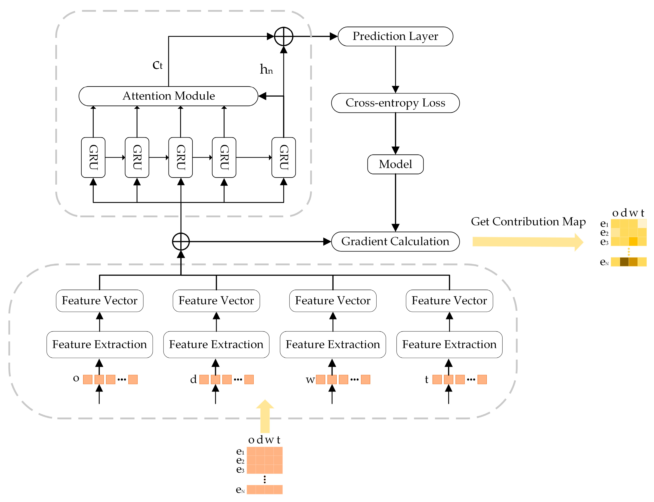
3.3. Saliency Methods Based on Gradient Information

In the field of computer vision, saliency methods based on gradient information, initially proposed by Karen Simonyan [40], serve as an interpretability tool. This method generates contribution maps to visually reveal the key features on which the model relies during the recognition or classification process. These features may include color, shape, texture, etc., which together form the basis of the model’s decision-making. The core of this method is that it only relies on a pre-trained classification model to complete the generation of the saliency map.
Simonyan’s research introduced two main techniques to explain the working principles of convolutional neural networks. One of them is the calculation of class contribution maps for specific images and categories. Specifically, the task takes an image I , a category c , and the model’s score for that category S c as input, and outputs a contribution map M that ranks the influence of each pixel in I on the score S c ( I ) . To illustrate, suppose there is a linear model for calculating the score of category c , which can be represented as follows:
S c ( I ) = w c T I + b c
In this context, I represents the vectorized representation of the image, and w c and b c are the model’s weight vector and bias, respectively. In this linear case, the magnitude of each element in the weight vector w directly reflects the importance of the corresponding pixel to category c . However, since the model’s predictions involve multiple layers of nonlinear transformations, the class score S c ( I ) is a highly nonlinear function of the image I , and thus the reasoning of the linear model cannot be directly applied. To approximate this relationship in deep networks, a first-order Taylor expansion is used within the neighborhood of the given image I 0 to approximate S c ( I ) , resulting in a linearized local representation as follows:
S c ( I ) w T I + b
This process involves the computation of the gradient, since w is the derivative of S c at point I 0 with respect to image I . The greater the absolute value of the gradient, the more significant the impact of the corresponding pixel on the classification results. Based on the principles outlined above, we can conclude that gradient information can, to some extent, reflect the model’s prediction process.
Based on the above principles, we can conclude that gradient information can reflect the prediction process of the model to a certain extent. Introducing this principle into the field of individual travel prediction, the input of the model is transformed into time series data containing multiple sequences and features, and the interpretability method outputs a gradient information matrix with the same dimension as the input. In this context, the gradient information represents the contribution of each sequence feature to the final travel prediction result. If the gradient information at a certain position is significantly higher than that at other positions, it means that the travel event at that moment has a decisive influence on the prediction.

4. Experiment

We have designed a series of experiments to explore the interpretability of gradient information across different time ranges by constructing models with varying sequence lengths. These models are based on the same network architecture, but the change in input sequence length allows us to analyze the temporal dependencies of key features in travel patterns and their impact on prediction results.
First, we build a travel prediction model based on an embedding layer, temporal processing layer, and attention layer as the platform for our interpretability study (Section 4.1). Next, we construct a mask matrix based on gradient information to quantify feature importance (Section 4.2) and introduce metrics used to assess the impact of the mask operation on model prediction behavior (Section 4.3). Finally, we investigate the specific contribution of features with different gradient magnitudes to the model’s prediction through feature importance evaluation (Section 4.4). These experimental designs and evaluation metrics will help us systematically validate the interpretability of gradient information in the travel prediction model and lay the foundation for subsequent experimental analysis.

4.1. Model Training

The model training process is based on subway card swipe data from a large city, involving a subway system composed of 91 subway stations. The data samples obtained contain travel records from approximately 200,000 passengers. According to the travel records of these passengers, a data set is constructed, and four characteristics of departure station number o, destination station number d, departure week w, and travel arrival time t are selected to construct a spatiotemporal travel record:
e = ( o , d , w , t )
In the feature processing stage, embedding techniques are employed to enrich the feature representation of individual travel records. For spatial attributes, such as subway station numbers, an embedding layer is used to map these discrete identifiers into a low-dimensional, dense vector space. Since the continuity of time does not directly reflect the numerical impact on travel predictions, the time attribute is first discretized into time points with categorical significance. For instance, a day is divided into several time intervals, and each interval is assigned an embedding vector. The core function of the embedding layer is to convert the discrete features in the travel records into continuous, high-dimensional vector representations. These vectors can capture the complex patterns and trends of individual travel behavior.
After the embedding layer, a time-series processing layer was introduced to model the periodicity and temporal dependencies of travel records. This layer receives the sequence of travel record embedding vectors generated by the embedding layer and outputs a series of hidden states to capture the temporal information in the sequence. Specifically, the input to the time-series processing layer is a series of embedding vectors, and this layer processes these vectors through a recurrent neural network or its variants (LSTM or GRU), outputting a series of hidden states h 1 , h 2 , , h N . Among these hidden states, h 1 , h 2 , , h N 1 is referred to as the candidate vector, representing the cumulative information of each time step in the sequence; q serves as the query vector for the calculation of attention weights in the next stage.
The attention layer constructs the context vector by meticulously capturing the similarity between the candidate vectors and the query vector. Specifically, a feedforward neural network (FNN) is utilized to transform each hidden state h t , yielding the corresponding nonlinear representations z t as follows:
z t = tanh ( W h t + b )
Here, t [ 1 , n 1 ] and n is the sequence length. W denotes the weight matrix, b represents the bias term, and tanh is the activation function, which introduces nonlinearity. After obtaining the nonlinear representations, the similarity between each z t and the query vector h t is calculated, serving as the basis for assigning attention weights. The calculation of attention weights α t can be expressed as follows:
α t = exp ( z t T h t ) t = 1 n 1 exp ( z t T h t )
Based on the calculated attention weights α t , the candidate vectors z t are weighted and summed to obtain the final context vector c t :
c t = t = 1 n 1 α t z t
The context vector c t integrates the information of all candidate vectors in the sequence, and this design enables the model to flexibly focus on the information that is most critical for prediction. The complete model training and interpretation process is shown in Figure 4.
To explore the differences in gradient information interpretation of travel prediction models under different sequence lengths, three different travel sequence lengths were chosen, namely 20, 40, and 60. Then, all travel samples were divided into training and testing sets in an 8:2 ratio.
In the example experiment, cross entropy is used as the loss function of model training, and accuracy is used as the evaluation index of model performance. The prediction performance of models with different lengths is as follows: without masking operations, modeling was carried out for three different sequence lengths (20, 40, 60), and the final prediction accuracy of the models is shown in Table 3.
The model achieved the highest accuracy (58.51%) on the test set with a sequence length of 40, which suggests that sequences of medium length may contain just enough information to capture the key features of travel patterns. Sequences that are too short may fail to provide sufficient contextual information to capture complex travel patterns, thus limiting the model’s predictive power. On the other hand, sequences that are too long may contain a substantial amount of redundant information, causing the model to overfit on unimportant details.

4.2. Mask Matrix

This section aims to investigate the importance of features in individual travel prediction models by constructing a mask matrix based on gradient information. Our methodology is based on the observation that gradients themselves provide a direct measure of feature contributions in the model’s decision-making process. The formula for calculating the gradient matrix is as follows:
G = S c x i , j
Here, G denotes the gradient matrix of the model’s output with respect to the original input matrix, where each element g i , j corresponds to the absolute value of the gradient of x i , j in the original input matrix X , indicating the gradient contribution of the i t h feature of the j t h sequence to the model’s output for category c .
Based on the gradient matrix G , we can identify the feature locations with the maximum gradient values and construct a mask matrix M . This matrix has the same shape as the original matrix X but only contains 0 and 1. The formula for constructing the mask matrix is the following:
M i , j = 1   if   g i , j = max k ( g i k )   0   otherwise
Here, M i , j is the element in the i t h row and j t h column of the mask matrix M , and g i , j is the corresponding element in the gradient matrix G . For each sample X , we identify the feature with the maximum gradient value among all features and set that position to 0 in the mask matrix, while setting all other positions to 1. The masked matrix can then be represented as follows:
X ˜ = X M
Theoretically, this masking method essentially shields key features in the travel data, thereby reducing the content of the corresponding travel records and exploring the impact of these features on the model’s predictions. The process of constructing the mask matrix is illustrated in Figure 5.

4.3. Benchmarking

The construction of a mask matrix based on gradient information helps us explore the role of gradient information in reducing the information content of travel records. To quantify the impact of this information reduction on the model’s predictive behavior, the following two evaluation metrics are proposed in this section:
  • Jensen–Shannon Divergence (JS): The Jensen–Shannon divergence is a metric for assessing the difference between two probability distributions. The formula for calculating the Jensen–Shannon divergence of the model’s output distribution is as follows:
    J S ( P   |   |   Q ) = 1 2 K L ( P   |   |   P + Q 2 ) + 1 2 K L ( Q   |   |   P + Q 2 )
Here, P and Q represent the probability distributions predicted by the original model and the masked model, respectively. The KL (Kullback–Leibler divergence) is used to measure the degree of difference between two probability distributions, with the formula given below:
K L ( P | | Q ) = x X P ( x )   l o g P ( x ) Q ( x )
Compared to the KL divergence, the JS divergence is symmetric and always returns a non-negative value. The JS divergence is zero if and only if P and Q are identical.
2.
Predictive Accuracy Difference Ratio (PA): PA is a metric that measures the decline in prediction accuracy when the model faces masked data. The formula for calculating PA is as follows:
P A = T o r i g i n a l T total T m a s k e d T total
Here, T o r i g i n a l represents the number of correct predictions by the model on the original data, T m a s k e d represents the number of correct predictions by the model on the masked data, and T total represents the total number of samples. If the value of PA is larger, it indicates that the feature has a greater contribution to the model’s prediction, or that the feature accounts for a larger amount of information in the model’s prediction. It should be noted that we only apply masking to samples predicted as positive examples. Randomly selecting samples might include some that the model already predicts incorrectly, and these samples already represent the model’s prediction errors.

4.4. Feature Impact Analysis

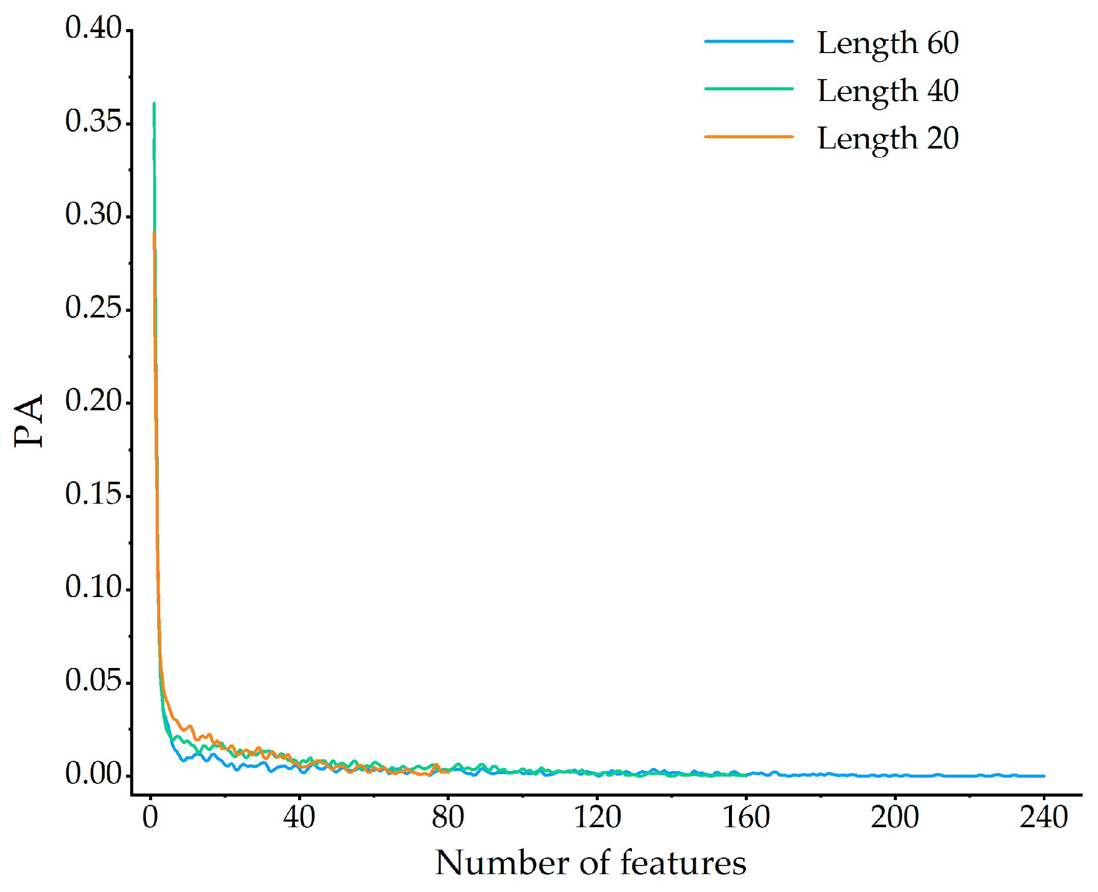
4.4.1. Analysis of Single-Feature Mask Results

We designed a single-feature masking experiment to investigate the impact of individual features on the model’s prediction performance. In the experiment, we randomly selected 1000 samples from the test set that were correctly predicted by the model. These samples covered different travel patterns and feature combinations, ensuring the representativeness and reliability of the experimental results. By ranking the gradient information, we were able to determine the influence of each sample feature on the model’s prediction. Then, we masked each feature position in the input data to simulate the absence of that feature in the prediction process. The results obtained are shown in Table 4.
Figure 6 illustrates the trend of changes in the model’s PA value when single features are masked in descending order. When the feature at the maximum gradient position was masked, the model’s JS divergence increased significantly, and the PA value also dropped substantially, with the model performance experiencing a sharp decline (by about one-third). This indicates that this feature point may be the most critical for prediction. Specifically, when this feature was masked, the model’s prediction accuracy decreased significantly, and the output probability distribution also changed markedly. This further confirms the central role of the maximum gradient feature in the model’s decision-making process. In addition to the maximum gradient feature, only the top few features had a noticeable impact on the prediction. These features may be the most recent travel features in the historical records, which provide important contextual information for the model, helping it better understand and predict future travel behavior. Masking these features also led to a significant downward trend in the model’s prediction accuracy, although the impact was slightly less than that of the maximum gradient feature.
For single features with smaller gradient values, masking these features had a relatively minor impact on the model, with a fluctuating downward trend. This suggests that as the gradient decreases, the feature’s impact on the model indeed diminishes, but not in a linear fashion. Specifically, if a single feature from a distant historical record does not contain key information for prediction or travel patterns, masking it would not cause a sharp decline in the model’s accuracy. This is because these features contribute little to the model’s prediction, and the model can rely on other unmasked features to maintain prediction performance. Masking distant historical features would not disrupt the model’s pattern information, as these features have a minor impact on the model’s prediction, and the model can rely on other unmasked features to maintain prediction performance.

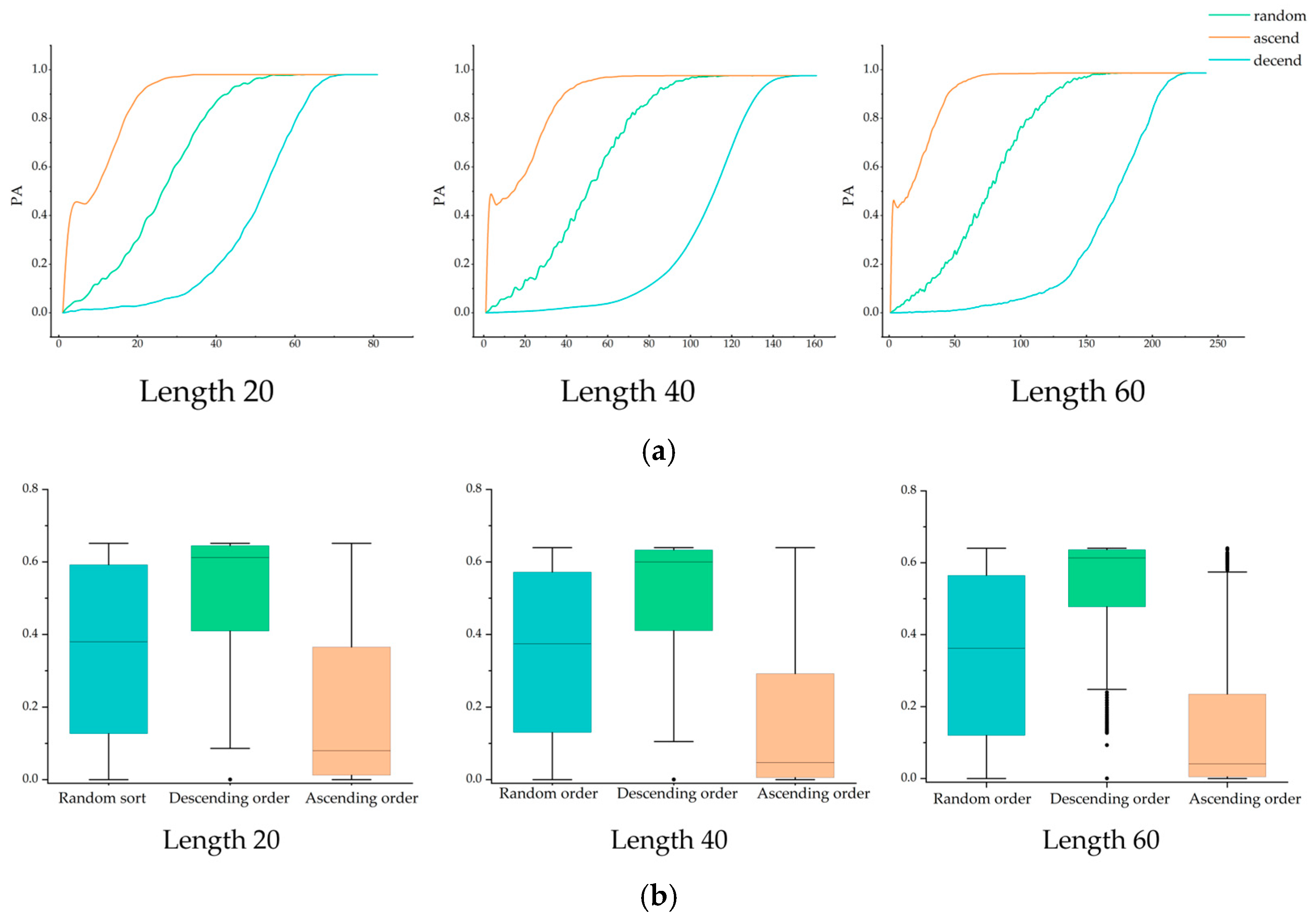
4.4.2. Comparison of Multi-Feature Masking Policies

The single-feature masking experiment preliminarily verified the effectiveness of gradient information in indicating feature importance. To gain a more comprehensive understanding of the contribution of each feature to the performance of the machine learning model, we further designed a multi-feature masking experiment. In the experiment, we ranked the features according to the gradient magnitude and adopted three different masking strategies: random-order masking, descending-order masking, and ascending order-masking. By observing the changes in model performance under different strategies, we can gain in-depth insights into the interactions between features and their combined impact on model predictions.
Under the random-order masking strategy, we randomly selected a certain number of features for masking, which does not take into account the gradient information of the features. Therefore, it can serve as a baseline experiment to compare the effects of the other two strategies. There are many similarities between the different sorting results for the three different sequence lengths as shown in Figure 7:
The descending-order masking strategy ranks and masks features in descending order of gradient values, forming different numbers of feature subsets until all features are masked. According to our hypothesis, these features contribute significantly to the model’s predictions, so masking them would have a noticeable impact on model performance. The experimental results confirmed this hypothesis. In the descending order strategy, with a very small subset of features masked, the PA value showed a rapid upward trend. This indicates that these prioritized masked feature combinations play a “core” role in the model, providing strong information for predictions, such as the commuting peak on weekdays or high-frequency travel patterns between specific stations. In the three different lengths, after a sharp increase, the PA value experienced a brief decline and then rose gently. This may be due to the model starting to adjust its weight and dependencies, shifting to using the remaining features for predictions. Although these features may not be as important as the initially masked ones, they still contain a certain amount of information that can help the model maintain a certain level of prediction performance. The changes in JS divergence values support this inference. The JS values in descending order are relatively high, indicating significant changes in the output distribution, which proves that the masked feature combinations with larger gradients have a greater impact on model performance.
Contrary to the descending order strategy, the ascending order masking strategy prioritizes masking features with smaller gradient values. The experimental results show that under this strategy, a larger feature masking subset is needed for the model performance to decline. One possible speculation is that the masking of non-important features in the early stage has a minor impact on model prediction performance. The JS distribution is lower because the masking of non-important features in the early stage has a low impact on model prediction performance. However, when the feature subset includes high-gradient features, the model’s JS divergence value will change dramatically, resulting in more outliers appearing above the box plot. This indicates that although low-gradient features have a limited impact on the model’s immediate predictions, they still support the model’s overall performance to a certain extent. Under the random masking strategy, the model’s prediction performance declines gradually, but at a relatively gentle pace. The distribution range of JS divergence values under this strategy is relatively large, possibly because the proportion of important features and non-important features masked under the random strategy is different. This shows that when features are randomly selected for masking, the model can adjust other unmasked features to maintain a certain level of prediction performance, indicating that the model has a certain degree of robustness.
In summary, we can draw the following conclusions: In individual travel prediction models, there is a significant difference in the contribution of features to model predictions. Features with larger gradient values have a more noticeable impact on model prediction performance, but this impact is not a simple linear relationship. The feature with the maximum gradient value has the greatest impact on model performance, causing a decline of about 30%; apart from the feature at the maximum gradient position, the impact of other features on model performance shows an upward and downward fluctuation and gradually decreases. This fluctuation may reflect the interactions between features and their complex impact on model predictions. A single feature cannot be a strong factor affecting the model, but specific feature combinations, especially those with larger gradient values, can have a significant impact on the model with a small feature masking subset. Additionally, the experimental results show that in the ascending order arrangement, the smallest feature masking subset (about 25% of the features) has a very limited impact on model predictions, with a decline in prediction accuracy of less than 20%. The subway travel prediction model has a certain degree of robustness and can resist the impact of feature loss to a certain extent; features with smaller gradient values have a relatively low contribution to the model. This means that when conducting feature selection or model optimization, it is possible to consider reducing the dependence on these features, thereby simplifying the model and improving efficiency.

5. Interpreting Predictions Using Contribution Maps

To further illustrate the interpretability of gradient information in individual travel prediction tasks, in this subsection, we will briefly explain how to reconceptualize the contribution map and use it for travel prediction tasks. By visualizing the gradient information, we demonstrate how the gradient information explains the model’s decision-making behavior from input to output. Figure 1, Figure 2, Figure 3 and Figure 4 display the model’s decision-making process for different travel patterns within the correctly observed subset.
Figure 8 shows the gradient information under the home-to-work travel pattern. The heatmap reveals a highly consistent travel pattern, which is clearly reflected in the gradient information. It can be seen from the figure that specific origin–destination (OD) pairs (such as 55–56 and 5655) reappear at multiple time points, indicating that passengers’ travel behavior is highly regular. Under this pattern, the model can easily capture these repetitive travel patterns, thus achieving high accuracy in predicting the next trip. The gradient information in this case is mainly concentrated on these repeatedly appearing OD pairs, showing high weights. This gradient distribution indicates that the model has high confidence in these regular patterns and therefore gives these patterns higher priority in prediction. Moreover, due to the regularity of the travel pattern, the model also has strong generalization ability when dealing with these data and can make accurate predictions even when facing a small amount of travel records. The gradient information under this pattern not only helps us understand the basis of the model’s predictions but also provides opportunities for optimizing the model, such as by reducing the dependence on these highly repetitive patterns and increasing the model’s adaptability to new emerging patterns.
Figure 9 shows the contribution map when an anomaly occurs in a regular travel pattern, revealing how the model handles this sudden change. It can be seen from the figure that although most of the travel patterns still follow the original regularity (the repeated appearance of 18–10 and 10–18), the appearance of station 80 breaks this regularity and shows a high gradient weight. This may be because the last two travel behaviors (18–80 and 10–18) provide two high-probability options for the next trip (18–10 and 18–80). The model regards station 80 as an important feature because it represents a potential change in passengers’ travel behavior. It also indicates that passengers’ next travel choices are not only influenced by their recent travel behavior but also by their past travel, which is in line with our common sense.
Figure 10 shows the contribution map when two anomaly stations appear in a regular travel pattern, displaying how the model deals with this more complex change. It can be seen from the figure that in addition to the original regular OD pairs (such as 81–14 and 14–81), the appearance of stations 3 and 35 increases the complexity of the travel pattern. This may be a home-work-supermarket-restaurant-home travel pattern, or it may be special activities or emergency matters on weekends. It can be seen from the contribution map that these two anomaly stations occupy high weights in the gradient information, which is also the sample where the maximum gradient position does not appear on the recent travel sequence in the example. This weight distribution may be because the model has identified a strong association between these stations and passengers’ travel purposes. This association makes the model very confident in its prediction, without the need to rely on other features, even though these stations do not often appear in passengers’ daily travel. This reflects the model’s attempt to balance the conflict between known regular travel patterns and newly emerging anomaly patterns, and to stick to its prediction under high confidence.
Figure 11 shows that even in the case of coexisting multiple travel patterns and seemingly no discernible pattern, the model can still make accurate predictions. In this situation, the model needs to extract useful information from a large number of travel records and identify the potential patterns hidden behind the messy data. It can be seen from the figure that although the travel patterns changed multiple times in the previous week, the model can identify some implicit patterns or trends by analyzing a large number of travel records, such as the frequent appearance of the 42–22 OD pair within specific time periods (eight or nine in the morning). These patterns are reflected in the gradient information, showing high weights. Compared with other samples, Figure 11 has a significant feature—the regular information in the historical records is assigned to higher weights, which is represented by brighter colors in the contribution map. The possible reason for this phenomenon is that although passengers’ travel behavior may show diversity and unpredictability in the long term, in the short term, some travel patterns may reappear and form recognizable regularities. The model maintains high prediction accuracy when facing complex travel data by identifying and reinforcing this regularity information. This ability enables the model to maintain stable prediction performance when facing changing passenger behavior.

6. Conclusions

This study is the first to transfer interpretability analysis methods from the field of image recognition to the domain of transportation travel, addressing the shortcomings of existing XAI methods in analyzing dynamic features of historical travel sequences. It systematically explores the interpretability value of gradient information in individual travel prediction models. Feature masking experiments based on real-world data show that gradient information effectively reveals the model’s decision logic, but the influence of features exhibits complex nonlinear relationships. Specifically, masking the maximum gradient feature position results in a performance decline of about 30%, while masking other features causes performance fluctuations and a decaying trend, indicating that the collaborative effect between features has a composite impact on the prediction results. Notably, masking 20% of high-gradient features leads to a 50% performance degradation, while masking 40% of low-gradient features results in only a 20% performance decline, confirming that the model is highly sensitive to core feature combinations and exhibits strong robustness to non-critical features.
We would like to point out several limitations of this study, which provide potential directions for future research. First, while gradient information performs well in explaining travel prediction model decisions, it remains an approximation of local linear relationships and thus struggles to fully capture the nonlinear decisions of deep neural networks. Second, contribution maps provide the extent and correlation of travel feature influences on the output result but cannot construct understandable causal chains or generate natural language explanations. Third, alternative variants based on gradient information have been proposed in the literature [41,42,43], and these variants have been applied in computer vision. Researching the performance of these alternatives in the context of travel prediction would be a productive direction for further study. Fourth, the experimental data is limited to a single scenario with medium-length sequences and does not cover the true complexity of multi-city, multi-modal features, which may cast doubt on the generalizability of the conclusions in longer periods or more dynamic scenarios. These limitations are both objective constraints on the current research and point to improvements for deepening interpretability studies.
To conclude, while our analysis indicates that the proposed gradient-based interpretability method provides a valuable tool for understanding the underlying principles of models in the context of travel prediction, it must be acknowledged that the proposed method does not fully solve the black-box problem of deep neural networks because it does not completely explain the inner workings. Future work could focus on developing multimodal interpretability frameworks integrating causal reasoning, establishing cross-domain interpretability evaluation standards, and building benchmark datasets that cover multiple scenarios and traffic feature scales, thereby advancing the practical implementation of explainable AI technologies in smart city decision-making systems.

Author Contributions

Conceptualization, Z.S., P.Z. and X.S.; methodology, Z.S. and P.Z.; software, Z.S. and Y.L.; validation, Z.S., P.Z. and X.S.; formal analysis, Z.S. and Y.L.; investigation, Z.S. and Y.L.; resources, Z.S. and X.S.; data curation, Z.S., P.Z. and X.S.; writing—original draft preparation, Z.S., P.Z. and X.S.; writing—review and editing, P.Z., X.S. and Y.L.; visualization, Z.S. and Y.L.; supervision, Z.S., P.Z. and X.S.; project administration, X.S.; funding acquisition, P.Z. All authors have read and agreed to the published version of the manuscript.

Funding

This research was supported by the Young Scientists Fund of the National Natural Science Foundation of China (12304240); key R&D and Promotion Project of Henan Province (Science and Technology Research) (242102210063); The Fundamental Research Fund of Henan Academy of Sciences (230620057); Natural Science Foundation of Henan (242300421456).

Institutional Review Board Statement

Not applicable.

Informed Consent Statement

Not applicable.

Data Availability Statement

The original contributions presented in the study are included in the article. Further inquiries can be directed to the corresponding author.

Acknowledgments

The authors are grateful to the colleagues and students who supported this study. Special thanks go to all participants in the user experiments for their valuable contributions. Their involvement and insights helped advance the study, providing foundational data that enriched our understanding of user perspectives on data privacy.

Conflicts of Interest

The authors declare no conflicts of interest.

References

  1. Guo, Q.; Lu, Q.; Liu, Z.; Yang, Z. Expressway toll station management and control decision-making system based on event feature machine learning. Highway 2025, 2, 312–318. [Google Scholar]
  2. Polson, N.G.; Sokolov, V.O. Deep learning for short-term traffic flow prediction. Transp. Res. Part C Emerg. Technol. 2017, 79, 1–17. [Google Scholar] [CrossRef]
  3. Sun, Y.; Jiang, Z.; Gu, J.; Zhou, M.; Li, Y.; Zhang, L. Analyzing high speed rail passengers’ train choices based on new online booking data in China. Transp. Res. Part C Emerg. Technol. 2018, 97, 96–113. [Google Scholar] [CrossRef]
  4. Ma, Z.; Zhang, P. Individual mobility prediction review: Data, problem, method and application. Multimodal Transp. 2022, 1, 100002. [Google Scholar] [CrossRef]
  5. Gilpin, L.H.; Bau, D.; Yuan, B.Z.; Bajwa, A.; Specter, M.; Kagal, L. Explaining explanations: An overview of interpretability of machine learning. In Proceedings of the 2018 IEEE 5th International Conference on Data Science and Advanced Analytics (DSAA), Turin, Italy, 1–4 October 2018; pp. 80–89. [Google Scholar]
  6. Huang, L.; Zheng, W.; Deng, Z. Tourism Demand Forecasting: An Interpretable Deep Learning Model. Tour. Anal. 2024, 29, 465–479. [Google Scholar] [CrossRef]
  7. Lundberg, S.M.; Lee, S.-I. A unified approach to interpreting model predictions. In Proceedings of the 31st International Conference on Neural Information Processing Systems (NIPS’17), Long Beach, CA, USA, 4–9 December 2017; Curran Associates Inc.: Red Hook, NY, USA, 2017; pp. 4768–4777. [Google Scholar]
  8. Ribeiro, M.T.; Singh, S.; Guestrin, C. “Why should I trust you?” Explaining the predictions of any classifier. In Proceedings of the 22nd ACM SIGKDD International Conference on Knowledge Discovery and Data Mining, San Francisco, CA, USA, 13–16 August 2016; pp. 1135–1144. [Google Scholar]
  9. Wang, S.; Ding, S.; Xiong, L. A new system for surveillance and digital contact tracing for COVID-19: Spatiotemporal reporting over network and GPS. JMIR mHealth uHealth 2020, 8, e19457. [Google Scholar] [CrossRef]
  10. Theissler, A.; Spinnato, F.; Schlegel, U.; Guidotti, R. Explainable AI for time series classification: A review, taxonomy and research directions. IEEE Access 2022, 10, 100700–100724. [Google Scholar] [CrossRef]
  11. Hu, L.; Wang, K. Computing SHAP Efficiently Using Model Structure Information. arXiv 2023, arXiv:2309.02417. [Google Scholar]
  12. Sushil. Interpreting the interpretive structural model. Glob. J. Flex. Syst. Manag. 2012, 13, 87–106. [Google Scholar] [CrossRef]
  13. Navada, A.; Ansari, A.N.; Patil, S.; Sonkamble, B.A. Overview of use of decision tree algorithms in machine learning. In Proceedings of the 2011 IEEE Control and System Graduate Research Colloquium, Shah Alam, Malaysia, 27–28 June 2011; pp. 37–42. [Google Scholar]
  14. Tang, L.; Xiong, C.; Zhang, L. Decision tree method for modeling travel mode switching in a dynamic behavioral process. Transp. Plan. Technol. 2015, 38, 833–850. [Google Scholar] [CrossRef]
  15. Jia, S.; Lin, P.; Li, Z.; Zhang, J.; Liu, S. Visualizing surrogate decision trees of convolutional neural networks. J. Vis. 2020, 23, 141–156. [Google Scholar] [CrossRef]
  16. Guo, M.; Ye, P.; Liu, X.; Xiong, G.; Zhang, L. An Interpretability Analysis of Travel Decision Learning in Cyber-Physical-Social-Systems. In Proceedings of the 2021 IEEE 1st International Conference on Digital Twins and Parallel Intelligence (DTPI), Beijing, China, 15 July–15 August 2021; pp. 340–343. [Google Scholar]
  17. Saputra, R.; Sihabuddin, A. Mobility Prediction Using Markov Models: A Survey. In Proceedings of the 2024 7th International Conference on Informatics and Computational Sciences (ICICoS), Semarang, Indonesia, 17–18 July 2024; pp. 508–513. [Google Scholar]
  18. Kumar, M.R.; Kamisetty, S.S.S.; Reddy, N. A robust approach for road traffic prediction using Markov chain model. In Proceedings of the 2023 Seventh International Conference on Image Information Processing (ICIIP), Solan, India, 22–24 November 2023; pp. 663–669. [Google Scholar]
  19. Chen, Y.; Jin, Z.; Li, C. Trip purpose prediction based on hidden Markov model with GPS and land use data. In Proceedings of the 2020 IEEE 5th International Conference on Intelligent Transportation Engineering (ICITE), Beijing, China, 11–13 September 2020; pp. 55–59. [Google Scholar]
  20. Jin, Z.; Chen, Y.; Li, C.; Jin, Z. Trip destination prediction based on hidden Markov model for multi-day global positioning system travel surveys. Transp. Res. Rec. 2023, 2677, 577–587. [Google Scholar] [CrossRef]
  21. Madsen, A.; Reddy, S.; Chandar, S. Post-hoc interpretability for neural NLP: A survey. ACM Comput. Surv. 2022, 55, 155. [Google Scholar] [CrossRef]
  22. Štrumbelj, E.; Kononenko, I. Explaining prediction models and individual predictions with feature contributions. Knowl. Inf. Syst. 2014, 41, 647–665. [Google Scholar] [CrossRef]
  23. Yin, G.; Huang, Z.; Fu, C.; Ren, S.; Bao, Y.; Ma, X. Examining active travel behavior through explainable machine learning: Insights from Beijing, China. Transp. Res. Part D Transp. Environ. 2024, 127, 104038. [Google Scholar] [CrossRef]
  24. Yang, Z.; Tianyuan, S.; Caiyun, Q. The impact of the built environment in the surrounding areas of Nanjing urban rail transit stations on residents’ activities—Analysis based on gradient boosting decision tree and SHAP interpretation model. Sci. Technol. Eng. 2023, 23, 7509–7519. [Google Scholar]
  25. Li, W.; Deng, A.; Zheng, Y.; Yin, Z.; Wang, B. Analysis of Residents’ Travel Mode Choice in Medium-sized City Based on Machine Learning. J. Transp. Syst. Eng. Inf. Technol. 2024, 24, 13–23. [Google Scholar]
  26. Slik, J.; Bhulai, S. Transaction-Driven Mobility Analysis for Travel Mode Choices. Procedia Comput. Sci. 2020, 170, 169–176. [Google Scholar] [CrossRef]
  27. Covert, I.; Lee, S.I. Improving kernelshap: Practical shapley value estimation using linear regression. In Proceedings of the International Conference on Artificial Intelligence and Statistics, Virtual, 13–15 April 2021; PMLR: New York, NY, USA; pp. 3457–3465. [Google Scholar]
  28. Bento, J.; Saleiro, P.; André, F.C.; Figueiredo, M.A.T.; Bizarro, P. TimeSHAP: Explaining Recurrent Models through Sequence Perturbations. In Proceedings of the 27th ACM SIGKDD Conference on Knowledge Discovery & Data Mining (KDD’21), Virtual, 14–18 August 2021; Association for Computing Machinery: New York, NY, USA, 2021; pp. 2565–2573. [Google Scholar]
  29. Balouji, E.; Sjöblom, J.; Murgovski, N.; Chehreghani, M.H. Prediction of Time and Distance of Trips Using Explainable Attention-based LSTMs. arXiv 2023, arXiv:2303.15087. [Google Scholar]
  30. Masampally, V.S.; Verma, R.; Mitra, K. Application of TimeSHAP, an explainable AI Tool, for Interpreting. In Optimization, Uncertainty and Machine Learning in Wind Energy Conversion Systems; Springer: Singapore, 2025; pp. 243–266. [Google Scholar]
  31. Jin, C.; Tao, T.; Luo, X.; Liu, Z.; Wu, M. S2N2: An Interpretive Semantic Structure Attention Neural Network for Trajectory Classification. IEEE Access 2020, 8, 58763–58773. [Google Scholar] [CrossRef]
  32. Ahmed, I.; Kumara, I.; Reshadat, V.; Kayes, A.S.M.; Heuvel, W.-J.v.D.; Tamburri, D.A. Travel time prediction and explanation with spatio-temporal features: A comparative study. Electronics 2021, 11, 106. [Google Scholar] [CrossRef]
  33. Vijaya, A.; Bhattarai, S.; Angreani, L.S.; Wicaksono, H. Enhancing Transparency in Public Transportation Delay Predictions with SHAP and LIME. In Proceedings of the 2024 IEEE International Conference on Industrial Engineering and Engineering Management (IEEM), Bangkok, Thailand, 15–18 December 2024; pp. 1285–1289. [Google Scholar]
  34. Srivastava, N.; Gohil, B.N. Ridership Trend Analysis and Explainable Taxi Travel Time Prediction for Bangalore Using e-Hailing. In Proceedings of the 7th International Conference of Transportation Research Group of India (CTRG 2023); Springer Nature: Berlin/Heidelberg, Germany, 2025; Volume 2, pp. 383–400. [Google Scholar]
  35. Zhang, P.; Koutsopoulos, H.N.; Ma, Z. DeepTrip: A deep learning model for the individual next trip prediction with arbitrary prediction times. IEEE Trans. Intell. Transp. Syst. 2023, 24, 5842–5855. [Google Scholar] [CrossRef]
  36. Feng, J.; Li, Y.; Zhang, C.; Sun, F.; Meng, F.; Guo, A.; Jin, D. Deepmove: Predicting human mobility with attentional recurrent networks. In Proceedings of the 2018 World Wide Web Conference, Lyon, France, 23–27 April 2018; pp. 1459–1468. [Google Scholar]
  37. Hosain, M.T.; Jim, J.R.; Mridha, M.F.; Kabir, M. Explainable AI approaches in deep learning: Advancements, applications and challenges. Comput. Electr. Eng. 2024, 117, 109246. [Google Scholar] [CrossRef]
  38. Linardatos, P.; Papastefanopoulos, V.; Kotsiantis, S. Explainable AI: A review of machine learning interpretability methods. Entropy 2020, 23, 18. [Google Scholar] [CrossRef]
  39. Mikolov, T.; Chen, K.; Corrado, G.; Dean, J. Efficient estimation of word representations in vector space. arXiv 2013, arXiv:1301.3781. [Google Scholar]
  40. Simonyan, K.; Vedaldi, A.; Zisserman, A. Deep Inside Convolutional Networks: Visualising Image Classification Models and Saliency Maps. arXiv 2013, arXiv:1312.6034. [Google Scholar]
  41. Sundararajan, M.; Taly, A.; Yan, Q. Axiomatic attribution for deep networks. In Proceedings of the International Conference on Machine Learning, Sydney, Australia, 6–11 August 2017; PMLR: New York, NY, USA; pp. 3319–3328. [Google Scholar]
  42. Shrikumar, A.; Greenside, P.; Kundaje, A. Learning important features through propagating activation differences. In Proceedings of the International Conference on Machine Learning, Sydney, Australia, 6–11 August 2017; PMLR: New York, NY, USA; pp. 3145–3153. [Google Scholar]
  43. Selvaraju, R.R.; Cogswell, M.; Das, A.; Vedantam, R.; Parikh, D.; Batra, D. Grad-cam: Visual explanations from deep networks via gradient-based localization. In Proceedings of the IEEE International Conference on Computer Vision, Venice, Italy, 22–29 October 2017; pp. 618–626. [Google Scholar]
Figure 1. Current mainstream interpreters (left) only calculate attributes of static features. Gradient based saliency methods (right) compute contributions across the entire input sequence.
Applsci 15 05269 g001
Figure 2. A visual comparison of interpretability frameworks.
Applsci 15 05269 g002
Figure 3. Mapping relationships between interpretability methods and models.
Applsci 15 05269 g003
Figure 4. Deep learning model architecture with GRU and attention mechanism for generating contribution maps.
Applsci 15 05269 g004
Figure 5. Construction method of mask matrix.
Applsci 15 05269 g005
Figure 6. Change of PA value of model after masking single-feature at different positions.
Applsci 15 05269 g006
Figure 7. (a) Line graph showing PA values after masking; (b) box plot presentation of JS values after masking.
Applsci 15 05269 g007
Figure 8. The predicted site label is 56.
Applsci 15 05269 g008
Figure 9. The predicted site label is 10.
Applsci 15 05269 g009
Figure 10. The predicted site label is 35.
Applsci 15 05269 g010
Figure 11. The predicted site label is 22.
Applsci 15 05269 g011
Table 1. Comparison of interpretability solutions in terms of explanation granularity and computational efficiency. Our method can be used for static feature and temporal feature interpretation and has linear computational efficiency O(N).
DimensionInterpretation GranularityComputational Efficiency
Decision treeStaticO(N)
KernelSHAPStaticO(2N)
TimeSHAPStatic and TemporalO(2N-i)
LIMEStaticO(N)
Gradient (ours)Static and TemporalO(N)
Table 2. Image processing terminology and travel prediction modeling equivalents.
Image Recognition TasksTravel Prediction Task
PixelFeature
Intensity SizeValue Size
Label CategoryOption/Forecast Target
Label SetOption Set
Table 3. Predictive accuracy of the model.
Sequence Length204060
Training Set Accuracy59.04%60.10%59.16%
Test Set Accuracy57.82%58.51%57.50%
Table 4. Changes in metrics after mask maxima for different sequence lengths.
Sequence LengthJSPA
200.08630.292
400.10500.361
600.09290.342
Disclaimer/Publisher’s Note: The statements, opinions and data contained in all publications are solely those of the individual author(s) and contributor(s) and not of MDPI and/or the editor(s). MDPI and/or the editor(s) disclaim responsibility for any injury to people or property resulting from any ideas, methods, instructions or products referred to in the content.

