Discrete Element Simulations of Damage Evolution of NiAl-Based Material Reconstructed by Micro-CT Imaging

Featured Application

A novel geometry reconstruction based on micro-CT imaging allows directly incorporating the microstructure of porous materials in discrete element simulations.

Abstract

Sintered porous materials present challenges for any modeling approach applied to simulate their damage evolution because of their complex microstructure, which is crucial for the initialization and propagation of microcracks. This paper presents discrete element simulations of the damage evolution of a NiAl-based material reconstructed by micro-CT imaging. A novel geometry reconstruction procedure based on micro-CT images and the adapted advancing front algorithm fills the solid phase using well-connected irregular and highly dense sphere packing, which directly represents the microstructure of the porous material. Uniaxial compression experiments were performed to identify the behavior of the NiAl sample and validate the discrete element model. Discrete element simulations based on micro-CT imaging revealed a realistic representation of the damage evolution and stress–strain dependency. The stress and strain of the numerically obtained curve peak differed from the experimentally measured values by 0.1% and 4.2%, respectively. The analysis of damage evolution was performed according to the time variation rate of the broken bond count. Investigation of the stress–strain dependencies obtained by using different values of the compression strain rate showed that the performed simulations approached the quasi-static state and achieved the acceptable accuracy within the limits of the available computational resources. The proposed stress scaling technique allowed a seven times increase of the size of the time step, which reduced the computing time by seven times.

1. Introduction

The numerical discrete element method (DEM) explicitly represents materials as assemblies of discrete particles or elements whose interactions dictate the overall behavior of the system [1]. In the DEM, each particle is assigned mass, geometry (which usually is as simple as a sphere [2] or a more complex shape [3]), and material properties, which are related to the contact interaction between particles governed by several contact laws. At the simplest level, the interaction is often modeled using an elastic spring, accompanied by tangential (shear) interaction with friction law [4]. To model solid materials, particles adhere to one another due to cohesive forces, assigning a cohesive bond between particles at the contact points. This approach is particularly suited for materials whose mechanical response is governed by the movement, contact, and breakage of individual grains or aggregates, such as granular soils [5], rocks [6], concrete [7], composites [8], and many other materials. Cohesive interactions enable crack initiation and propagation simulation by defining bonds that resist tensile and shear forces until failure [9]. When the force across a bond exceeds a critical value, the bond is broken, thereby simulating the initiation of microdamage. The accumulation of such breakages can eventually lead to macroscopic fracture. Recently, such an approach of modeling damage evolution by using DEM has been utilized widely [10].

Concrete fracture phenomena and their statistically varying character were investigated in [11], examining the complex processes of failure mechanisms, crack propagation, and damage evolution using the 2D discrete element model. In [12], a three-dimensional DEM particle-based cohesive crack model was developed to model the mixed-mode fracture process of brittle materials, aiming to simulate the material transition from a solid phase to a particulate phase. Damage and fatigue crack growth simulation of quasi-brittle materials were performed using a continuum damage model implemented in a discrete element code [13]. In [14], shale disk samples were studied under Brazilian test conditions using a 3D digital image correlation system (DIC) together with an inherently anisotropic model established within a DEM framework. Damage evolution and crack propagation of more advanced material, a fiber composite, was simulated in [8] concerning various fracture modes, such as fiber–matrix debonding, ply-to-ply delamination, matrix cracking, and fiber rupture. Thus, various DEM models are not limited to the analysis of granular materials, but can be effectively applied to studying cohesive powders [15], sea ice failure [16], the hardening/softening behavior of soil [17], starch agglomerates [18], high temperature resistant concrete [19], and coupled multi-physical problems [20].

Despite the efficiency of the mentioned DEM models in predicting the damage evolution of brittle materials, they are formulated based on regular/spherical discrete elements, which do not have any physical representations and were utilized only as the meshing structural feature. In the last several years, we can find more sophisticated approaches aimed at representing the damage of materials consisting of microstructural objects, such as grains [21,22] or aggregates [23,24,25,26]. The micro objects can be modeled as Voronoi polyhedra designed to resemble grains [21], accounting for the grain-scale heterogeneity observed in natural granular rocks. Grain-scale heterogeneity reproduced by Voronoi tessellation has also been discussed in [22]. Most of these grain-scale models exploit several reconstruction techniques to obtain the actual representation of the material microstructure, starting from optical microscopy [21,27] and ending with X-ray micro-computed tomography (micro-CT) imaging [23,24,26]. The exact arrangement of structural features, such as grains, particles, fibers, pores, or additional phases is crucial in the context of microcracking initialization and subsequent propagation. Micro-CT involves analyzing microstructural images to capture the complete 3D distribution of material components [28]. With a spatial resolution of up to 100 nm and the ability to scan objects as large as 200 mm in diameter, X-rays provide precise, slice-by-slice mapping of the sample.

This proposed paper takes the advantage of integrating DEM simulation with micro-CT imaging, showing significant potential in the modeling of fracture behavior and damage evolution of complex porous materials manufactured by the powder metallurgy route. A bonded particle model, formulated in Section 2.1, has been employed to reproduce the deformation and final degradation of a porous nickel aluminide (NiAl) sample during a uniaxial compression test. The details of the experimental measurements have been provided in Section 2.2. The novel reconstruction procedure of the porous sample microstructure based on micro-CT images and the adapted advancing front algorithm have been outlined in Section 2.3. Section 3 discusses the results of the DEM simulations, and the conclusions are given in Section 4.

2. Materials and Methods

2.1. Formulation of the Discrete Element Model

Compared with continuum-based methods, the significant advantages of the DEM are the ease of introducing discontinuities with little computational effort and the possibility to model highly complex systems using the simple laws on individual particles without any predispositions to where cracks may occur and propagate.

2.1.1. Governing Relations of the Discrete Element Method

The DEM governs a system, which can be considered an assembly of discrete particles interacting with one another in the frame of Newtonian mechanics. An arbitrary particle i in the system of N particles undergoes translational and rotational motion as follows:

$$m_i{\displaystyle \frac{d^2{x}_i}{d{t}^2}}=F_i, I_i{\displaystyle \frac{d{\omega }_i}{dt}}=M_i,$$

(1)

where t is time, and m_i and I_i are the mass and the moment of inertia of the particle, respectively, while the vectors x_i and ${\omega }_i$ determine the position of the center of the particle i and the rotational velocity around the particle’s center of mass. The vectors F_i and M_i represent the resultant force and the resultant moment, acting in the center of the particle i. Equation (1), along with the specified initial conditions, presents a universal mathematical model, capturing a large amount of problems encountered by the DEM and various extensions.

The forces acting on the particle may be classified into the forces induced by the external fields, the contact forces between the contacting particles, and the bond forces between the bonded particles. Thus, the resultant force can be expressed by the external forces, the sum of the contact forces $F_{ij}^c$ between the contacting particles that are indicated by subscript j = 1, N_c, and by the sum of the bond forces $F_{ik}^b$ between the bonded particles that are indicated by subscript k = 1, N_b:

$$F_i=m_{i}g+{\displaystyle \sum _{j=1,j\ne i}^{N_c}{F}_{ij}^c}+{\displaystyle \sum _{k=1,k\ne i}^{N_b}{F}_{ik}^b},$$

(2)

where g is the acceleration due to gravity. Thus, in the present work, the electromagnetic force, the aerodynamic force, and other external forces [29], except for the gravity force, are not considered.

The rotational motion is governed by the respective moments. The moment of the particle i can be restricted by the contribution of moments $M_{ij}^c$ of the contacting particles and by the contribution of moments $M_{ik}^b$ of the bonded particles:

$$M_i={\displaystyle \sum _{j=1,j\ne i}^{N_c}{M}_{ij}^c}+{\displaystyle \sum _{k=1,k\ne i}^{N_b}{M}_{ik}^b}.$$

(3)

In the case of granular flows, there are no bonded particles, therefore, N_b, $F_{ik}^b$, and $M_{ik}^b$ are always equal to zero. In the case of the media discretized by the bonded particles, both counterparts can be not equal to zero. The moment and the force acting between two particles i and j can be expressed as the sum of the normal and tangential components:

$$F_{ij}^o=F_{ij,n}^o+F_{ij,t}^o,$$

(4)

$$M_{ij}^o=M_{ij,n}^o+M_{ij,t}^o,$$

(5)

where $F_{ij,n}^o$ and $F_{ij,t}^o$ are the normal and tangential vector components of the force acting between the particles i and j, and $M_{ij,n}^o$ and $M_{ij,t}^o$ are the normal and tangential components of the moment, respectively. The superscript o can be equal to c and b in the case of the granular flows and the bonded particles, respectively.

2.1.2. The Bonded Particle Model

The bonded particle model, based on a parallel bond [9], is implemented to numerically simulate the uniaxial vertical compression of NiAl samples. The parallel bond can be envisioned as a set of elastic springs uniformly distributed over the circular cross-section in 3D, lying on the contact plane and centered on the contact point. Thus, parallel bonds can transmit both the force and the moment between the bonded particles. When the parallel bond is formed between the particles i and j, the contact force and the moment are initialized to zero. Each subsequent increment of relative displacement and relative rotational velocity produces the increments of the force and the moment that are added to the current values. Thus, in each time step l + 1, the normal bond force $F_{ij,n}^{b,l+1}$ and the tangential bond force $F_{ij,t}^{b,l+1}$ can be obtained, adding the increments of the normal bond force $\Delta F_{ij,n}^{b,l+1}$ and the tangential bond force $\Delta F_{ij,t}^{b,l+1}$ to the normal contact force $F_{ij,n}^{b,l}$ and the tangential contact force $F_{ij,t}^{b,l}$ of the previous time step l, respectively:

$$F_{ij,n}^{b,l+1}=F_{ij,n}^{b,l}+\Delta F_{ij,n}^{b,l+1}=F_{ij,n}^{b,l}+k_{ij,n}^{b}A\Delta u_{ij,n}^{l+1},$$

(6)

$$F_{ij,t}^{b,l+1}=F_{ij,t}^{b,l}+\Delta F_{ij,t}^{b,l+1}=F_{ij,t}^{b,l}-k_{ij,t}^{b}A\Delta u_{ij,t}^{l+1},$$

(7)

where A is the cross-sectional area of the bond, and $k_{ij,n}^b$ and $k_{ij,t}^b$ denote the normal and the tangential stiffness of the bond, while $\Delta u_{ij,n}^{l+1}$ and $\Delta u_{ij,t}^{l+1}$ are the increments of the relative normal displacement and the relative tangential displacement during the time step l + 1, respectively.

In each time step l + 1, the normal moments $M_{ij,n}^{b,l+1}$ and the tangential moments $M_{ij,t}^{b,l+1}$, as well as their increments $\Delta M_{ij,n}^{b,l+1}$ and $\Delta M_{ij,t}^{b,l+1}$, are computed as follows:

$$M_{ij,n}^{b,l+1}=M_{ij,n}^{b,l}+\Delta M_{ij,n}^{b,l+1}=M_{ij,n}^{b,l}-k_{ij,t}^{b}J\Delta {\theta }_{ij,n}^{l+1},$$

(8)

$$M_{ij,t}^{b,l+1}=M_{ij,t}^{b,l}+\Delta M_{ij,t}^{b,l+1}=M_{ij,t}^{b,l}-k_{ij,n}^{b}I\Delta {\theta }_{ij,t}^{l+1},$$

(9)

where $M_{ij,t}^{b,l}$ and $M_{ij,t}^{b,l}$ are the current values of the normal and tangential components of the moment at the previous time step l, respectively, and $\Delta {\theta }_{ij,n}^{l+1}$ and $\Delta {\theta }_{ij,t}^{l+1}$ are the increments of the normal and tangential components of the relative rotational velocity at the time step l + 1, respectively, while I and J are the moment of inertia and the polar moment of inertia of the parallel bond’s cross-section, respectively.

The parallel bonds break instantaneously when the maximum tensile stress ${\sigma }_{ij}^{\max }$ exceeds the tensile strength ${\sigma }_c$ or the maximum shear stress ${\tau }_{ij}^{\max }$ exceeds the shear strength ${\tau }_c$, leading to microcrack formation between the two particles. The expressions of the maximum tensile stress and the maximum shear stress, acting on the bond, are derived from the beam bending theory, which gives the criteria of the bond failure formulated as

$${\sigma }_c<{\sigma }_{ij}^{\max }={\displaystyle \frac{-F_{ij,n}^b}{A}}+{\displaystyle \frac{\left|M_{ij,t}^b\right|}{I}}R,$$

(10)

$${\tau }_c<{\tau }_{ij}^{\max }={\displaystyle \frac{\left|F_{ij,t}^b\right|}{A}}+{\displaystyle \frac{\left|M_{ij,n}^b\right|}{J}}R,$$

(11)

where R is the bond radius and $F_{ij,n}^b$ is the scalar value of the normal component of the bond force, which can cause bond breakage only in the case of tension. The bond is broken such that a microscopic crack is created to represent the failure of the material at this particular bond. The above consideration is very useful for explicitly simulating the initiation of spontaneous and random microscopic cracks in a brittle material, because there is no need to artificially describe any microscopic flaws and cracks at the beginning of a numerical simulation. Other details and the implementation of the bonded particle model can be found in [9,19].

2.1.3. The Computation of the Forces and Moments for Granular Flows

After the breakage of the bonds, contacting particles interact according to the granular flow model. Moreover, parallel bonds (6–9) act in parallel with the granular portion of the force–displacement behavior, when the depth of the overlap between the particles is more than zero. Thus, the implemented granular flow model is outlined as follows. In the case of granular flows, a model for the normal contact force depends on the contact geometry and the properties of the particle’s material. In general, the normal contact force $F_{ij,n}^c$ can be expressed as the sum of the elastic ($F_{ij,n,elastic}$) and viscous components. The elastic counterpart of the normal contact force is computed according to the formula as follows:

$$F_{ij,n,elastic}={\displaystyle \frac{k_{i,n}^p{k}_{j,n}^p}{k_{i,n}^p+k_{j,n}^p}}{\delta }_{ij,n}{n}_{ij},$$

(12)

where $n_{ij}$ is the unit normal vector, ${\delta }_{ij,n}$ is the depth of the overlap between the particles i and j in the normal direction, and $k_{i,n}^p$ and $k_{j,n}^p$ are the normal stiffnesses of the contacting particles i and j, respectively.

The computation of the tangential contact force is more complex, since the phenomena of tangential deformation, as well as static and dynamic friction, have to be considered. The most popular approach comprises the evolution of the tangential contact force $F_{ij,t}^c$ divided into the parts of static friction $F_{ij,t,static}$ and dynamic friction $F_{ij,t,dynamic}$:

$$F_{ij,t}^c=-t_{ij} min\left(\left|F_{ij,t,static}\right|,\left|F_{ij,t,dynamic}\right|\right),$$

(13)

The dynamic friction force is directly proportional to the normal component of the contact force:

$$F_{ij,t,dynamic}=-\mu \left|F_{ij,n}\right|t_{ij},$$

(14)

where $t_{ij}$ is the unit vector of the tangential contact direction and µ is the friction coefficient. The static friction force $F_{ij,t,static}$ can be calculated by summing up the elastic counterpart $F_{ij,t,elastic}$ and the viscous damping counterpart. The elastic counterpart of static friction can be obtained as follows:

$$F_{ij,t,elastic}=-{\displaystyle \frac{k_{i,t}^p{k}_{j,t}^p}{k_{i,t}^p+k_{j,t}^p}}\left|{\delta }_{ij,t}\right|t_{ij},$$

(15)

where $\left|{\delta }_{ij,t}\right|$ is the length of the tangential displacement, while $k_{i,t}^p$ and $k_{j,t}^p$ are the tangential stiffnesses of the contacting particles i and j, respectively.

Finally, the moment of the interacting particles (3) is computed as follows:

$$M_{ij}^c=d_{cij}\times F_{ij}^c,$$

(16)

where d_cij is the vector pointing from the particle’s center to the contact center. The details and implementation of the outlined granular flow model can be found in the refs. [9,30,31].

2.2. Preparation of NiAl Sample for DEM Simulations

The discrete element model was verified by the experimental results of a uniaxial compression test of a cube-shaped sample. Nickel aluminide was selected as a representative porous material. The NiAl sample was manufactured using the powder metallurgy technique based on Spark Plasma Sintering (SPS), related to resistive heating in an electrically conductive matrix. Densification of the material occurs at elevated temperatures in the presence of uniaxial pressure. The process of material compaction occurs due to diffusive mass transport mechanisms because of the generated Joule heat, which is a consequence of the flow of electric current through the usually graphite punches and dies [32]. This type of heating allows for high heating rates (up to 1000 °C/min), lower sintering temperatures, and much shorter processing times than conventional methods [33]. The method can effectively synthesize materials from metallic, ceramic, and composite powders [34,35].

Nickel aluminide (NiAl—Goodfellow) gas-atomized powders with an average particle size of 10 μm diameter and purity of 99.9% were selected for sintering. The main advantage of the SPS process is that it reduces uncontrolled grain growth at elevated temperatures and avoids undesirable structural changes when sintering reactive materials. The details of the manufacturing procedure are presented in [28]. The powder was loosely filled into a graphite die with an inner diameter of 26.0 mm and closed tightly with graphite punches. Graphite foil that was 0.5 mm thick was used as a die–powder spacer. Then, the NiAl powder was heated at a rate of 100 K/min to the target sintering temperature, reaching 1200 °C for a sintering time of 10 min. The sintering process conducted in a vacuum atmosphere was supported by an external pressure of 5 MPa. Afterwards, the samples were naturally cooled down. The final 25.0 mm diameter discs were cut and ground for further investigations. The density of the sintered materials was estimated using the Archimedes method. The average density of the NiAl material sintered in presented conditions was determined from 10 measurements and was 4620 kg/m³. This represents 78.1% of relative density, assuming a theoretical density of 5910 kg/m³.

To reconstruct the actual microstructure of the NiAl sample, the X-ray computed tomography (micro-CT) was carried out by the EasyTom system (RX Solutions (Chavanod, France)) using an open transmission X-ray source with a tungsten target and a diamond window at the tube voltage of 160 kV. The CT was performed for the sample volume of 2 × 2 × 2 mm³ with a voxel size of about 1.8 µm. In total, 2880 projections were taken using a PaxScan 2520DX Varian (Varex Imaging (Salt Lake City, UT, USA)) flat panel detector. The images were acquired in the continuous cone beam single circle acquisition mode with an additional 32 reference images.

Finally, the NiAl sample was subjected to the uniaxial compression test at room temperature using a Zwick Roell Z005 (ZwickRoell (Ulm, Germany)) universal testing machine equipped with a 1 kN force transducer. The experiments were conducted under displacement control with a strain rate of 10⁻³ s⁻¹. The tests were performed on cubic-shaped samples of 2 × 2 × 2 mm³ (Figure 1).

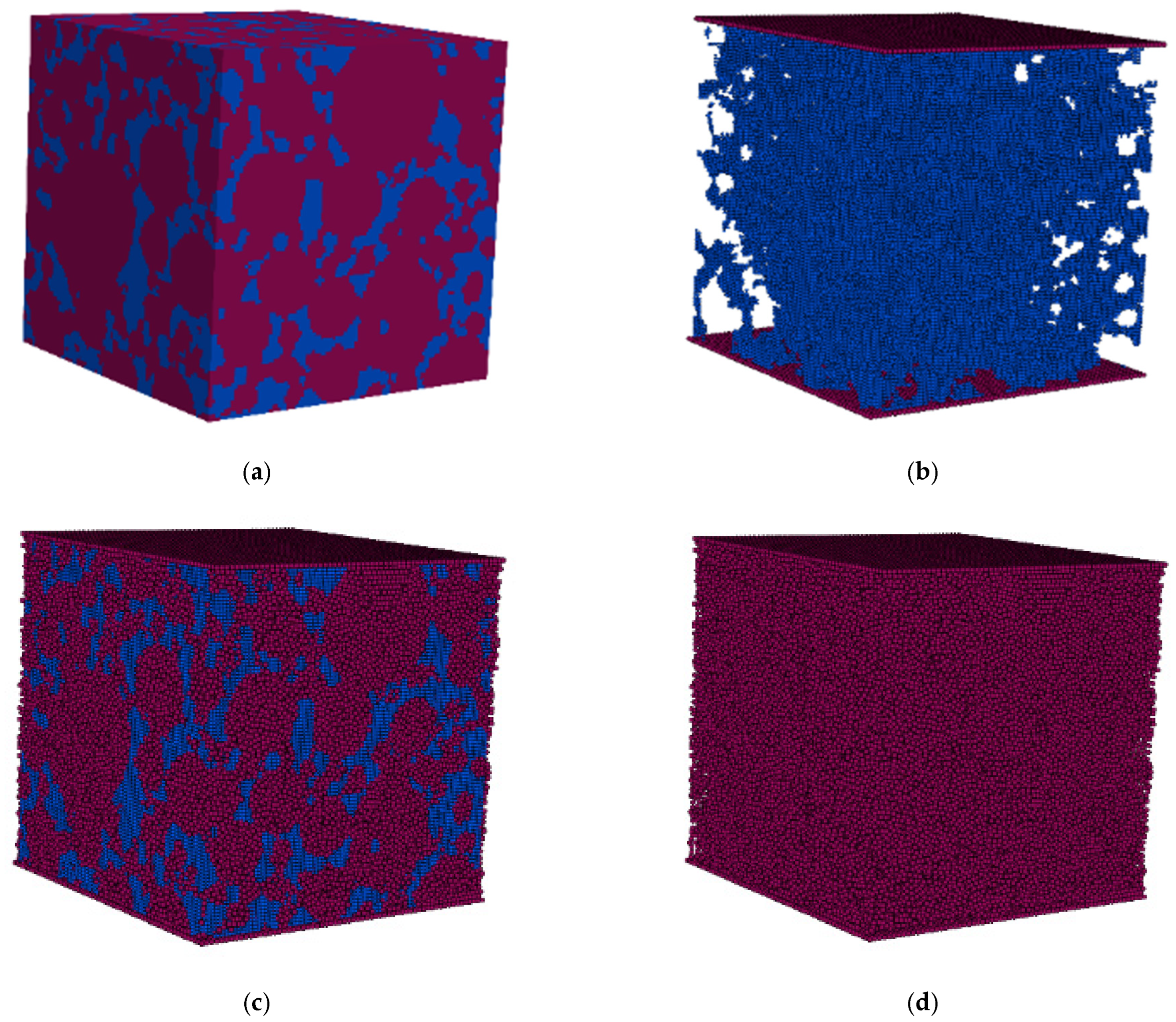
2.3. Development of a Geometrical Model of the NiAl Microstructure Based on Micro-CT Images

A geometrical model, realistically representing the material microstructure, is especially important because the properties of the material strongly depend on the particle packing used. Generation of a well-connected densely packed irregular assembly of particles is the key to successful DEM simulations. In the present research, particle packings of porous NiAl material are generated by the adapted advancing front algorithm according to micro-CT images. The proposed reconstruction procedure of the porous NiAl microstructure consists of four main steps, illustrated in Figure 2:

• Process the micro-CT scan for geometrical reconstruction of the NiAl sample (Figure 2a).
• Define the boundaries of the solid phase by the particles (Figure 2b).
• Fill the volume of the solid phase by irregular highly dense particle packing (Figure 2c).
• Remove the temporal particles from the pores (Figure 2d).

In the first step, the geometry of the NiAl sample is reconstructed by segmenting micro-CT images. Defining the representative volume element (RVE) also requires careful consideration to ensure statistical homogeneity of the microstructural elements (solid and pores). Based on the homogeneity analysis of sintered NiAl, we selected a sample comprising 100 × 100 × 100 voxels (183 × 183 × 183 μm³). Confirmation of the reliability of the images obtained is provided by the high agreement of the sinter porosity obtained by density measurement and volumetric image analysis, 21.8% and 21.9%, respectively. The solid and pore phases are identified by using phase masks and applying the threshold value. Figure 2a shows the segmented 3D model obtained from processing the initial micro-CT scan.

In the second step, the boundaries of the solid phase are defined by the particles. Pores are regularly filled by temporal particles of equal size (blue particles in Figure 2b). Each particle is placed in a voxel center of the micro-CT scan. Naturally, the accuracy of pore geometry is limited by the voxel size. The top and bottom boundaries of the sample are represented by regularly located particles (red particles in Figure 2b) to obtain smooth boundary surfaces that are loaded by moving two rigid plates during simulations. In our experience, rough surfaces produced by irregular packing of particles cause intensive initiation of microcracks on the loaded boundary, which might lead to premature sample failure. Other boundaries of the sample are traditionally represented by using planes, which causes rough surfaces formed from irregularly located particles in the final packing.

In the third step, the volume of the solid phase is filled by irregularly packed particles of defined size or radius distribution. A well-connected highly dense sphere packing (Figure 2c) is generated by using the adapted advancing front algorithm [36] for filling arbitrarily complex geometries.

In the fourth step, regularly packed particles are removed from the pores. These temporal particles were generated to define surfaces between the pores and solid phase in the second step. The generated porous NiAl sample of 183 × 183 × 183 μm³ is represented by an assembly of 188,190 irregularly packed particles of radius 1.5 μm (Figure 2d, Dataset S1).

The radius of particles is not strictly limited by the voxel size, which is a great advantage of the proposed geometry reconstruction procedure. A larger size of particles allows performing simulations of the considered RVE with a smaller number of particles, which can significantly shorten the computing time. This advantage is crucial for DEM simulations based on micro-CT images, because the material microstructure often requires high resolution images, leading to a large number of particles. In the present research, the diameter of the particles was larger than the voxel size by 64%, which allowed achieving acceptable accuracy of simulations within the limits of available computational resources.

The proposed reconstruction is based on the collection of voxels representing the exact microstructure of the NiAl sample. The characteristics of the grains (size, shape, and distribution) are the same in the preparation of 2D scans, creation of the 3D model defined as the collection of 2D scans, segmentation procedure, and final particle packing (Figure 2). It can be noticed the powder particles or grains have a spherical shape after sintering, with sizes ranging from several to tens of micrometers. NiAl grains are connected by small necks, which are also reproduced by micro-CT analysis as important microstructural features. Finally, the porosity can be characterized by an open type at the same level as the experimental one. All of the mentioned microstructural issues lead us to conclude that the modeling has been carried out on real experimental data, reflecting the representative state of the material in a reliable way.

3. Results and Discussion

A numerical investigation of the deformation and damage evolution of the NiAl sample was conducted using discrete element analysis based on micro-CT imaging. A large number of particles and small time steps make micro-CT-based DEM computations very time consuming. Naturally, parallel computing is perceived as an obvious way to increase computational capabilities. However, the selection of an efficient parallel algorithm is highly dependable on the considered problem and the method used [37,38,39]. Double-precision DEM computations were performed using the developed GPU code [19] on the NVIDIA^® Tesla™ P100 GPU Computing Accelerator. Geometry reconstruction, DEM simulation, and visualization of results were performed on the computational infrastructure [39] of the Vilnius Gediminas Technical University.

A uniaxial compression test of a cube-shaped NiAl sample was simulated using the developed discrete element model based on micro-CT imaging. The NiAl sample of 183 × 183 × 183 μm³ was represented by an assembly of 188,190 particles of radius 1.5 μm (Figure 2d). The irregularly packed sample was subjected to slow uniaxial vertical compression by moving two rigid plates. The compression strain rate was 53 s⁻¹, which was found to be sufficiently low to obtain quasi-static loading. In other directions, the deformations are free.

The main material properties of NiAl were measured in the experimental research. The parameters of the DEM model were considered as follows. The density of the NiAl particles is equal to 5910 kg/m³. Poisson’s ratio of NiAl is equal to 0.3; therefore, the ratios of normal to shear stiffness of the particles and bonds are considered equal to 3.0. The friction coefficient of the NiAl particles is assumed equal to 0.3. According to initial calibrations, the elasticity moduli of the particles and bonds are equal to 25 × 10⁹ Pa, which results in the slope angle of the numerically obtained stress–strain curve being close to that of the experimentally measured one. The normal stiffness of the bond is computed by using the values of the bond elasticity modulus and radii of bonded particles [9]. The tangential stiffness of the bond is obtained by dividing the normal bond stiffness by 3.0, because of the relevant Poisson’s ratio value. In the normal and tangential directions, the bond strength values are equal to 3 × 10⁸ Pa and 3 × 10⁹ Pa, respectively. According to the initial calibrations, carefully selected bond strength values have a crucial influence on the accurate prediction of the stress peak and following fall-down of the macroscopic stress–strain curve. The greatest challenge is to capture small deviations of the stress–strain curve from the line, avoiding premature fall-down of the curve. In such a complex case, typical of the slightly ductile behavior of materials, calibration of the bond strength values might be required to correct the value of the bond elasticity modulus, which governs the slope angle of the numerical stress–strain curve.

3.1. Stress–Strain Dependency and Comparison with the Experimental Measurements

DEM simulations of the uniaxial compression test were performed to obtain numerical results as close as possible to the experimentally measured response of the NiAl sample. The macroscopic response of the sample subjected to uniaxial compression load is represented by the stress–stain dependency. The total force of particles on the compressing plate is divided by the area of the sample to compute the stress values. The average strain is obtained by dividing the prescribed displacement of either the upper or lower compressing plates by the initial height of the sample. Figure 3 shows the quantitative comparison of the numerical results with the experimental measurements.

Figure 3a presents the stress dependency on strain obtained from the experimental uniaxial compression test (the curve “EXP”) and that obtained from DEM computations (the curve “DEM”). Three snapshots of particles colored according to their percentage of broken bonds at different stages of loading are included. Figure 3b presents the count of broken bonds, which describes the damaging process and supplements the stress–strain curve. During the performed simulations, the count of broken bonds N_bb increases from 0 to 19,504. In the generated discrete element packing, the total count of bonds is equal to 441,954.

Initially, when the strain varies from 0.000 to 0.010, the count of broken bonds is negligibly small (Figure 3b). Therefore, the elastic behavior of the material is dominant, and the numerical stress–strain curve is linear (Figure 3a). When the strain rises from 0.010 to 0.0261, the count of broken bonds exponentially increases (Figure 3b) and some random microcracks initiate (the second snapshot in Figure 3a), which leads to slow weakening of the sample. The macroscopic stress–strain curve starts deviating from the line, but only small differences can be observed (Figure 3a). In this strain interval, the experimental stress–strain curve shows some features of ductile behavior. However, the low value of the index B15 [40], equal to 0.51%, indicates more brittle behavior of the considered NiAl material. Finally, when the strain values exceed 0.0261, the count of broken bonds grows very quickly (Figure 3b) and macroscopic tensile cracks form in the sample (the third snapshot in Figure 3a). The macroscopic stress–strain curve falls down, indicating the beginning of the sample failure (Figure 3a). DEM simulations accurately predict the highest stress in the stress–strain curve. The difference between the numerically and experimentally obtained values does not exceed 0.213 MPa, which is less than 0.1% of the highest experimentally measured stress value. However, the strains of the stress peaks obtained numerically and experimentally differ by a significant value, equal to 0.0011, which is 4.2% of the experimentally measured strain.

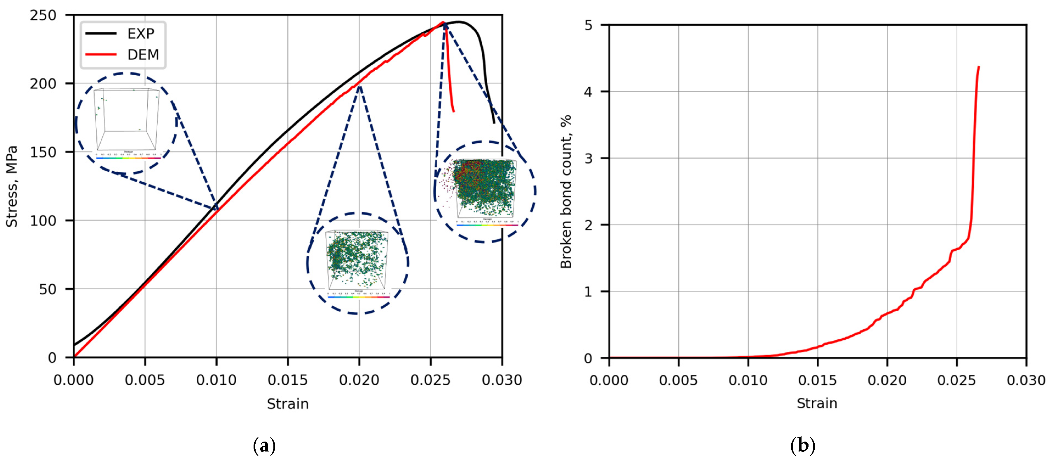
3.2. Analysis of Damage Evolution

Figure 4 shows the distribution of broken bonds visualized by particles colored according to their percentage of broken bonds. The count of broken bonds divided by the count of total bonds is employed as a data attribute of each particle to visualize damaged zones of the sample, where particles become weakly tied to their neighbors. In order to better examine the differences between the crack propagations, the frontal surface is segmented by horizontal and vertical planes that intersect in the center of the surface. The resulting four regions are numbered as follows: “I”, “II”, “III”, and “IV”. According to Figure 4, four time intervals, [t₁; t₂], [t₂; t₃], [t₃; t₄], and [t₄; t₅], are considered, where t₁ = 1.0 × 10⁻⁵ s, t₂ = 1.9 × 10⁻⁵ s, t₃ = 2.4 × 10⁻⁵ s, t₄ = 2.5 × 10⁻⁵ s, and t₅ = 2.6 × 10⁻⁵ s. In Figure 4a,b, orange ellipsoids and polygons mark some cracks that do not propagate in time period [t₂; t₃]. Red arrows show the main shear-dominated microcracks, whose lengths are more than four times larger than the distance between the centers of particles.

Crack propagation can be investigated taking into account the time variation rate of the broken bond count. In the time interval [t_i; t_j], it can be computed by using the formula ${\displaystyle \frac{{∆N}_{bb}}{∆t}}={\displaystyle \frac{N_{bb}\left(t_j\right)-N_{bb}\left(t_i\right)}{t_j-t_i}}$, where the difference of the broken bond count ∆N_bb is divided from the time interval length ∆t. The proposed indicator is relevant to the average propagation speed of a unit length crack in micromechanics. In the first time interval [t₁; t₂] of 9 µs, the strain rises from 0.010 to 0.0197 (Figure 4a), while the count of broken bonds increases from 54 to 2740. The time variation rate of the broken bond count is equal to 305 1/µs, which indicates the time interval of slow microcrack propagation. In the second time interval [t₂; t₃] of 5 µs, the strain grows from 0.0197 (Figure 4a) to 0.025 (Figure 4b), while N_bb increases from 2740 to 7147. The time variation rate of the broken bond count increases till 881 1/µs, which is 2.9 times faster than that in the above introduced time interval of slow microcrack propagation. Thus, it can be called the time interval of medium microcrack propagation. Since individual bonds have a discrete nature, the microcracks formed in the neighborhood are also discrete and might be not connected.

In the third time interval [t₃; t₄] of 1 µs, the strain grows from 0.025 (Figure 4b) to 0.0261 (Figure 4c), while N_bb increases from 7147 to 9146. The time variation rate of the broken bond count reaches 2028 1/µs, which is 6.7 times faster than that in the time interval of slow microcrack propagation and 2.3 times faster than that in the time interval of medium microcrack propagation. Figure 4c shows the formation of macrocracks that are mainly concentrated in the left upper region “I”. Therefore, it can be considered as the time interval of microcrack transfer to macrocracks. In the fourth time interval [t₄; t₅] of 1 µs, the strain rises from 0.0261 (Figure 4c) to 0.0271 (Figure 4d), which leads to the fastest growth of the broken bond count, from 9146 to 19,453. The time variation rate of the broken bond count equals 10,307 1/µs, which is 5.1 times faster than that in the previous time interval of microcrack transfer to macrocracks. Macrocrack propagation is caused by the high increase of the broken bond count in the whole macrocrack propagation volume; therefore, the last interval can be called the time interval of fast macrocrack propagation.

We made a detailed qualitative analysis of the accumulation of shearing cracks. While the strain level is less than 0.010, a negligibly small amount of bonds are broken and no detailed analysis of cracks is required. However, as the uniaxial compression load increases, multiple new microcracks initiate, propagate, and eventually coalesce into longer macrocracks. The initiation, accumulation, and propagation of shearing microcracks can be observed in the left upper region “I”, as presented in Figure 4a–d. At the end of the time interval of slow microcrack propagation, seven microcracks are already detected in this region (Figure 4b). Five microcracks are detected on the right upper surface region numbered by “II” at the end of the time interval of medium microcrack propagation, shown in Figure 4b. However, in the time interval of fast macrocrack propagation, the number of observed microcracks reaches ten and twelve, as presented in Figure 4c,d, respectively. Figure 4c,d shows that, during the time interval of fast macrocrack propagation, the smallest increase of microcrack number is observed in the bottom right surface region “III”. Different crack propagation in different regions is caused by asymmetrical distribution of material pores, directly implemented in the discrete element packing by using the micro-CT scan. Figure 4c,d shows that the main macroscopic shearing cracks form during the time interval of microcrack transfer to macrocracks, and propagate during the time interval of fast macrocrack propagation in the surface regions “I” and “IV” of the sample. Some macroscopic cracks suddenly propagate, leading to final failure of the sample. It is worth noting the fragmentation of the sample into more than two parts, which is common to failure patterns observed in uniaxial compression experiments of brittle materials.

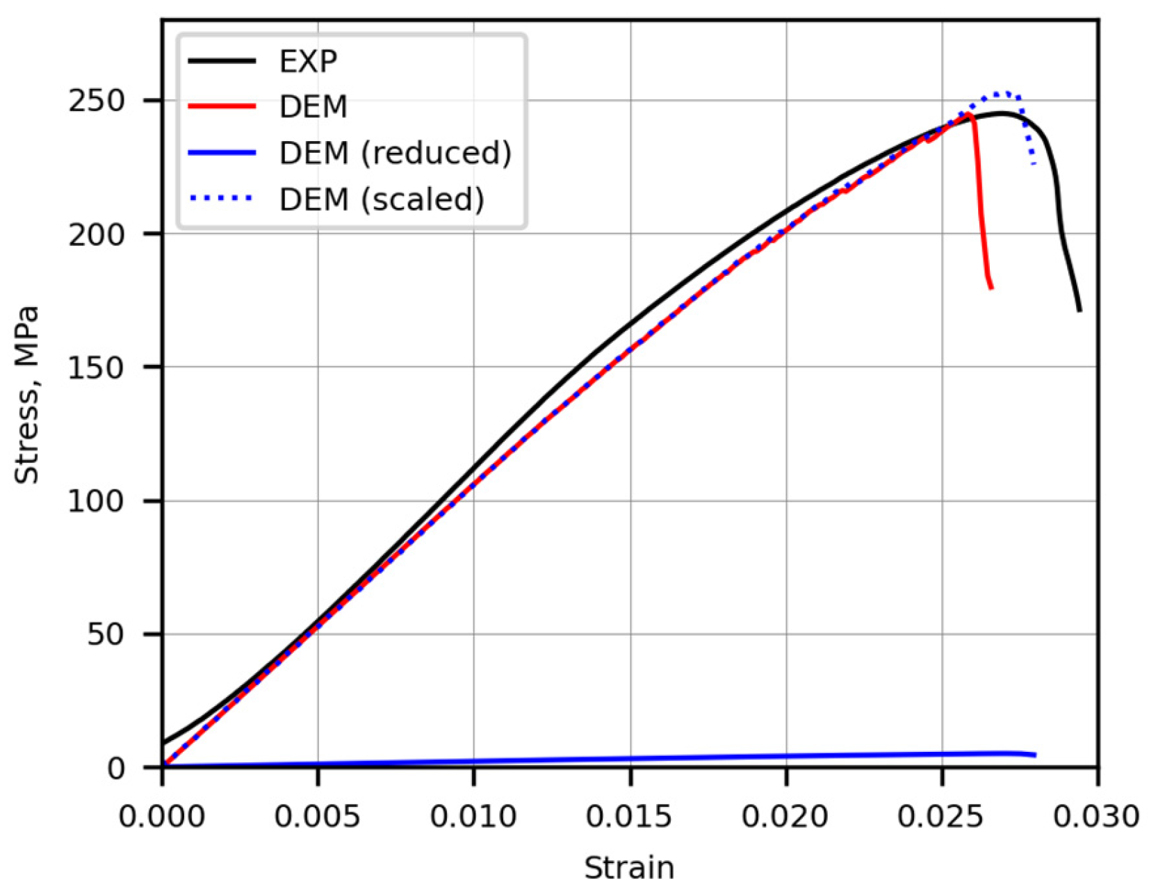
3.3. Proposed Stress Scaling Technique

Scaling of DEM parameters according to similarity conditions allows increasing the size of the time step constrained by an explicit numerical time integration scheme, which can substantially reduce computing time. It is shown that two models will obey the same governing Equation (1) if they satisfy the major similarity condition for DEM [41]:

$${\displaystyle \frac{m_1{l}_1}{F_1{t}_1^2}}={\displaystyle \frac{m_2{l}_2}{F_2{t}_2^2}}$$

(17)

where l₁, m₁, t₁, and F₁ and l₂, m₂, t₂, and F₂ are the characteristic length, mass, time, and force of models 1 and 2, respectively. For the considered mechanical system, only three dimensions are independent. If $l_1=l_2$, $m_1=m_2$, $t_1=t_2$, and $F_{sc}=F_1/sc$, then

$${\displaystyle \frac{{sc·F}_1}{sc}}={sc·F}_{sc}={sc·\sigma }_{sc}·A_{sc}={\sigma }_1·A_1=F_1$$

(18)

where sc is the scaling factor, $F_{sc}$ is the force magnitude computed with scaled-down values of parameters, ${\sigma }_{sc}$ is the stress computed with scaled-down values of parameters, and $A_{sc}$ is the characteristic area of the scaled model, which is proportional to the square of the characteristic length and equal to $A_1$. Thus, it is necessary to multiply the stresses of the scaled model from the scaling factor in order to get the stresses of the model with the original values of the parameters. In the present research, the values of the elastic moduli and bond breakage parameters (10–11) are scaled down by the scaling factor.

Figure 5 shows the accuracy of the proposed scaling technique. The curves “EXP” and “DEM” represent the stress dependency on strain obtained from the experimental uniaxial compression test and that attained from DEM computations with the original values of parameters, respectively. The curve “DEM (reduced)” represents the DEM computations with 50 times reduced values of elastic moduli and bond breakage parameters (10–11). The curve “DEM (scaled)” is the stress–strain curve of “DEM (reduced)”, for which the stresses are scaled 50 times. It is worth noting that DEM computations with 50 times reduced values of parameters can be performed with a $\sqrt{50}=7.07$ times larger time step. Thus, DEM computations with the reduced values of parameters lasted seven times shorter than those with the original values of parameters. When the strain rises from 0.010 to 0.0261, the curves “DEM” and “DEM (scaled)” almost coincide, which proves the high accuracy of the proposed scaling technique up to the time interval of fast macrocrack propagation, leading to the beginning of the sample failure. However, the stress peaks of the curves “DEM” and “DEM (scaled)” differ by 7.92 MPa, which is 3.2% of the highest stress value obtained in DEM computations with the original values of parameters. Thus, the accuracy of scaling requires further research in the case of fast macrocrack propagation and the sample failure.

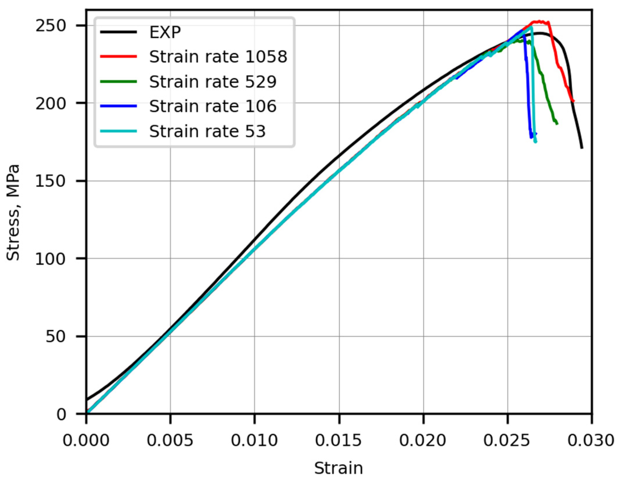
3.4. Compression Strain Rate for Quasi-Static Loading

Usually, in the experimental uniaxial compression test, the velocity of the compressing plates is lower than that in DEM simulations because of computing time limitations. However, computations performed with inappropriately high values of compression velocity, which can be expressed by the strain rate, are not able to properly simulate the quasi-static nature of the compression process.

Figure 6 presents the stress dependencies on strain obtained by using different values of the compression strain rate that vary from 53 s⁻¹ to 1058 s⁻¹. The curve “EXP” obtained from the experimental measurements is plotted for completeness reasons. All curves obtained for different values of the compression strain rate almost coincide up to the strain value of 0.025, which indicates the end of the time interval of medium microcrack propagation. However, some differences can be observed for higher strain values closer to the stress peaks. Thus, the compression strain rate can influence the numerical results in the time intervals of microcrack transfer to macrocracks and fast macrocrack propagation. The curve obtained by using the highest value of the compression strain rate, which equals 1058 s⁻¹, highly differs from the other curves. However, the differences between the curves obtained by using the small values of 53 s⁻¹ and 106 s⁻¹ can be treated as negligible. Thus, the computations performed by using the compression strain rate, which is close to 53 s⁻¹, approach the quasi-static state and achieve the acceptable accuracy within the limits of available computational resources.

4. Conclusions

In the present paper, the damage evolution of the porous NiAl material is simulated by using the DEM and the micro-CT imaging-based reconstruction of the material microstructure. Based on the performed geometry reconstruction, DEM simulations, and analysis of damage evolution, some observations and concluding remarks may be drawn as follows:

• The DEM supplemented by the micro-CT imaging-based reconstruction of the porous NiAl microstructure revealed a realistic representation of the damage evolution and stress–strain curve.
• While the count of broken bonds was negligibly small, the elastic behavior of the material was dominant, and the numerical stress–strain curve was linear.
• When the strain increased, the count of broken bonds exponentially grew, and some random microcracks initiated, which led to slow weakening of the sample and small deviations of the macroscopic stress–strain curve from the line.
• At the end of the investigated strain interval, the formation and propagation of macroscopic cracks caused the fall-down of the stress–strain curve, which indicated the beginning of the sample failure. The numerically obtained stress and strain of the curve peak differed from the experimentally measured values by 0.1% and 4.2%, respectively.
• At a high compression load, the propagation of macrocracks, caused by a high increase of the broken bond count in the whole macrocrack propagation volume, led to fragmentation of the sample into more than two parts, which is common to failure patterns observed in uniaxial compression experiments of brittle materials.
• The developed stress scaling technique, based on scaled-down elastic moduli with bond breakage parameters and scaled-up stress values, allowed a seven times increase of the size of the time step, which reduced the computing time by seven times. The proposed scaling was very accurate until the time interval of fast macrocrack propagation. However, the stress peaks of the original and scaled curves differed by 3.2% of the highest stress obtained in DEM computations with the original values of parameters.
• The analysis of stress–strain dependencies obtained by using different values of the compression strain rate showed that the computations performed with a compression strain rate close to 53 s⁻¹ approached the quasi-static state and achieved acceptable accuracy within the limits of the available computational resources.

References

1. Xu, Z.; Wan, Y.; Xin, D.; Zhao, Y.; Zhou, D. Discrete element numerical simulation of the effect of river ice porosity on impact force at bridge abutments. Appl. Sci. 2025, 15, 1738. [Google Scholar] [CrossRef]
2. Wang, Y.; Yu, S.; Wang, R.; Ding, B. The vibration response characteristics of neighboring tunnels induced by shield construction. Appl. Sci. 2025, 15, 1729. [Google Scholar] [CrossRef]
3. Wang, S.; Xu, Q.; Liang, D.; Ji, S. A novel discrete element method for smooth polyhedrons and its application to modeling flows of concave-shaped particles. Int. J. Numer. Methods Eng. 2024, 126, e7628. [Google Scholar] [CrossRef]
4. Cundall, P.A.; Strack, O.D.L. A discrete numerical model for granular assemblies. Géotechnique 1979, 29, 47–65. [Google Scholar] [CrossRef]
5. Jiang, M.; Zhang, A.; Shen, Z. Granular soils: From DEM simulation to constitutive modeling. Acta Geotech. 2020, 15, 1723–1744. [Google Scholar] [CrossRef]
6. Xia, M. Thermo-mechanical coupled particle model for rock. Trans. Nonferrous Met. Soc. China 2015, 25, 2367–2379. [Google Scholar] [CrossRef]
7. Wang, P.; Gao, N.; Ji, K.; Stewart, L.; Arson, C. DEM Analysis on the Role of Aggregates on Concrete Strength. Comput. Geotech. 2020, 119, 103290. [Google Scholar] [CrossRef]
8. Le, B.D.; Dau, F.; Charles, J.L.; Iordanoff, I. Modeling damages and cracks growth in composite with a 3D discrete element method. Compos. Part B Eng. 2016, 91, 615–630. [Google Scholar] [CrossRef]
9. Potyondy, D.O.; Cundall, P.A. A bonded-particle model for rock. Int. J. Rock Mech. Min. Sci. 2004, 41, 1329–1364. [Google Scholar] [CrossRef]
10. Chen, X.; Peng, D.; Morrisey, J.P.; Ooi, J.Y. Comparative assessment and unification of bond models in DEM simulations. Granul. Matter 2022, 24, 29. [Google Scholar] [CrossRef]
11. Beckmann, B.; Schicktanz, K.; Curbach, M. Discrete element simulation of concrete fracture and crack evolution. Beton-Und Stahlbetonbau 2018, 113, 91–95. [Google Scholar] [CrossRef]
12. Chen, H.; Zhang, Y.X.; Zhu, L.; Xiong, F.; Liu, J.; Gao, W. A particle-based cohesive crack model for brittle fracture problems. Materials 2020, 13, 3573. [Google Scholar] [CrossRef] [PubMed]
13. Gao, X.; Koval, G.; Chazallon, C. A discrete element model for damage and fatigue crack growth of quasi-brittle materials. Adv. Mater. Sci. Eng. 2019, 2019, 6962394. [Google Scholar] [CrossRef]
14. Yang, S.Q.; Yin, P.F.; Huang, Y.H. Experiment and Discrete Element Modelling on Strength, Deformation and Failure Behaviour of Shale Under Brazilian Compression. Rock Mech. Rock Eng. 2019, 52, 4339–4359. [Google Scholar] [CrossRef]
15. Tykhoniuk, R.; Tomas, J.; Luding, S.; Kappl, M.; Heim, L.; Butt, H.J. Ultrafine cohesive powders: From interparticle contacts to continuum behaviour. Chem. Eng. Sci. 2007, 62, 2843–2864. [Google Scholar] [CrossRef]
16. Long, X.; Ji, S.; Wang, Y. Validation of microparameters in discrete element modeling of sea ice failure process. Part. Sci. Technol. 2019, 37, 550–559. [Google Scholar] [CrossRef]
17. Xiang Bo, X.; Wang, X.J. A cohesive strengthening/damage-plasticity model and its application for DEM numerical investigation in hardening/softening of rock and soil. Comput. Geotech. 2023, 159, 105500. [Google Scholar] [CrossRef]
18. Horabik, J.; Wiącek, J.; Parafiniuk, P.; Stasiak, M.; Bańda, M.; Kobyłka, R.; Molenda, M. Discrete element method modelling of the diametral compression of Starch Agglomerates. Materials 2020, 13, 932. [Google Scholar] [CrossRef]
19. Pacevič, R.; Kačeniauskas, A. The performance analysis of the thermal discrete element method computations on the GPU. Comput. Inform. 2022, 41, 931–956. [Google Scholar] [CrossRef]
20. Baniasadi, M.; Baniasadi, M.; Peters, B. Coupled CFD-DEM with heat and mass transfer to investigate the melting of a granular packed bed. Chem. Eng. Sci. 2018, 178, 136–145. [Google Scholar] [CrossRef]
21. Xu, T.; Fu, T.-F.; Heap, M.J.; Meredith, P.G.; Mitchell, T.M.; Baud, P. Mesoscopic damage and fracturing of heterogeneous brittle rocks based on three-dimensional polycrystalline discrete element method. Rock Mech. Rock Eng. 2020, 53, 5389–5409. [Google Scholar] [CrossRef]
22. Li, X.F.; Li, H.B.; Liu, L.W.; Liu, Y.Q.; Ju, M.H.; Zhao, J. Investigating the crack initiation and propagation mechanism in brittle rocks using grain-based finite-discrete element method. Int. J. Rock Mech. Min. Sci. 2020, 127, 104219. [Google Scholar] [CrossRef]
23. Jin, C.; Yang, X.; You, Z. Automated real aggregate modelling approach in discrete element method based on X-Ray computed tomography images. Int. J. Pavement Eng. 2017, 18, 837–850. [Google Scholar] [CrossRef]
24. Suchorzewski, J.; Tejchman, J.; Nitka, M. Discrete element method simulations of fracture in concrete under uniaxial compression based on its real internal structure. Int. J. Damage Mech. 2018, 27, 578–607. [Google Scholar] [CrossRef]
25. Xue, B.; Pei, J.; Zhou, B.; Zhang, J.; Li, R.; Guo, F. Using random heterogeneous DEM model to simulate the SCB fracture behavior of asphalt concrete. Constr. Build. Mater. 2020, 236, 117580. [Google Scholar] [CrossRef]
26. Suchorzewski, J.; Nitka, M. Size effect at aggregate level in microCT scans and DEM simulation—Splitting tensile test of concrete. Eng. Fract. Mech. 2022, 264, 108357. [Google Scholar] [CrossRef]
27. Nguyen, N.H.T.; Bui, H.H.; Kodikara, J.; Arooran, S.; Darve, F. A discrete element modelling approach for fatigue damage growth in cemented materials. Int. J. Plast. 2019, 112, 68–88. [Google Scholar] [CrossRef]
28. Nosewicz, S.; Jurczak, G.; Wejrzanowski, T.; Ibrahim, S.H.; Grabias, A.; Węglewski, W.; Kaszyca, K.; Rojek, J.; Chmielewski, M. Thermal conductivity analysis of porous NiAl materials manufactured by spark plasma sintering: Experimental studies and modelling. Int. J. Heat Mass Transf. 2022, 194, 123070. [Google Scholar] [CrossRef]
29. Liu, G.; Marshall, J.S.; Li, S.Q.; Yao, Q. Discrete element method for particle capture by a body in an electrostatic field. Int. J. Numer. Methods Eng. 2010, 84, 1589–1612. [Google Scholar] [CrossRef]
30. Džiugys, A.; Peters, B. An approach to simulate the motion of spherical and non-spherical fuel particles in combustion chambers. Granul. Matter 2001, 3, 231–266. [Google Scholar] [CrossRef]
31. Kačeniauskas, A.; Kačianauskas, R.; Maknickas, A.; Markauskas, D. Computation and visualization of discrete particle systems on gLite-based grid. Adv. Eng. Softw. 2011, 42, 237–246. [Google Scholar] [CrossRef]
32. Wiśniewska, M.; Laptev, A.M.; Marczewski, M.; Krzyżaniak, W.; Leshchynsky, V.; Celotti, L.; Szybowicz, M.; Garbiec, D. Towards homogeneous spark plasma sintering of complex-shaped ceramic matrix composites. J. Eur. Ceram. Soc. 2024, 44, 7139–7148. [Google Scholar] [CrossRef]
33. Laptev, A.M.; Bram, M.; Vanmeensel, K.; Gonzalez-Julian, J.; Guillon, O. Enhancing efficiency of field assisted sintering by advanced thermal insulation. J. Mater. Process. Technol. 2018, 262, 326–339. [Google Scholar] [CrossRef]
34. Guillon, O.; Gonzalez-Julian, J.; Dargatz, B.; Kessel, T.; Schierning, G.; Räthel, J.; Herrmann, M. Field-assisted sintering technology/Spark plasma sintering: Mechanisms, materials, and technology developments. Adv. Eng. Mater. 2014, 16, 830–849. [Google Scholar] [CrossRef]
35. Santanach, J.G.; Weibel, A.; Estournès, C.; Yang, Q.; Laurent, C.; Peigney, A. Spark plasma sintering of alumina: Study of parameters, formal sintering analysis and hypotheses on the mechanism(s) involved in densification and grain growth. Acta Mater. 2011, 59, 1400–1408. [Google Scholar] [CrossRef]
36. Roselló, R.; Pérez, I.; Vanmaercke, S.; Recarey Morfa, C.; Cortés, L.; Casañas, H. Modified algorithm for generating high volume fraction sphere packings. Comput. Part. Mech. 2015, 2, 161–172. [Google Scholar] [CrossRef]
37. Govender, N. Study on the effect of grain morphology on shear strength in granular materials via GPU based discrete element method simulations. Powder Technol. 2021, 387, 336–347. [Google Scholar] [CrossRef]
38. Zheng, Z.; Zang, M.; Chen, S.; Zeng, H. A GPU-based DEM-FEM computational framework for tire-sand interaction simulations. Comput. Struct. 2018, 209, 74–92. [Google Scholar] [CrossRef]
39. Bystrov, O.; Pacevič, R.; Kačeniauskas, A. Performance of communication-and computation-intensive Saas on the OpenStack cloud. Appl. Sci. 2021, 11, 7379. [Google Scholar] [CrossRef]
40. Decheng, Z.; Ranjith, P.G.; Perera, M.S.A. The brittleness indices used in rock mechanics and their application in shale hydraulic fracturing: A review. J. Pet. Sci. Eng. 2016, 143, 158–170. [Google Scholar] [CrossRef]
41. Wang, Y.; Mora, P.; Liang, Y. Calibration of discrete element modeling: Scaling laws and dimensionless analysis. Particuology 2022, 62, 55–62. [Google Scholar] [CrossRef]
Figure 1. NiAl sample subjected to uniaxial compression at (a) the beginning of the loading stage (initial state), and (b) the end of the loading stage (damaged state).
Applsci 15 05260 g001
Figure 2. Reconstruction of NiAl sample geometry based on micro-CT imaging: (a) segmented micro-CT scan; (b) boundaries of the solid phase defined by the particles; (c) volume of the solid phase filled by irregularly located red particles; (d) final particle packing of the porous NiAl sample.
Applsci 15 05260 g002
Figure 3. Comparison of the numerical results with the experimental measurements: (a) the macroscopic stress–strain curves; (b) the percentage of broken bonds.
Applsci 15 05260 g003
Figure 4. Visualization of crack propagation over time: (a) t2 = 1.9 × 10⁻⁵ s, strain ε = 0.0197; (b) t3 = 2.4 × 10⁻⁵ s, strain ε = 0.025; (c) t4 = 2.5 × 10⁻⁵ s, strain ε = 0.0261; (d) t5 = 2.6 × 10⁻⁵ s, strain ε = 0.0271.
Applsci 15 05260 g004
Figure 5. The accuracy of the proposed scaling technique.
Applsci 15 05260 g005
Figure 6. Stress–strain dependencies obtained by using different values of the compression strain rate.
Applsci 15 05260 g006
Disclaimer/Publisher’s Note: The statements, opinions and data contained in all publications are solely those of the individual author(s) and contributor(s) and not of MDPI and/or the editor(s). MDPI and/or the editor(s) disclaim responsibility for any injury to people or property resulting from any ideas, methods, instructions or products referred to in the content.