Dynamic Heterogeneous Search-Mutation Structure-Based Equilibrium Optimizer

Abstract

Aiming at the issues of population diversity attenuation, insufficient search efficiency, and susceptibility to a local optimum in the equilibrium optimizer (EO), a dynamic heterogeneous search-mutation structure-based equilibrium optimizer (DHSMEO) is developed. First of all, a dynamic dual-subpopulation adaptive grouping strategy is constructed to boost population diversity, and it provides an effective information-exchange structure for the heterogeneous hybrid search strategy. Then, a heterogeneous hybrid search-based concentration-updating strategy is integrated to enhance search efficiency. Finally, a dynamic Levy mutation-based optimal equilibrium candidate-refining strategy is incorporated to strengthen the capability of escaping local optima. The optimization capability of DHSMEO is evaluated using 39 typical benchmark functions, and the experimental results validate its effectiveness and superiority. Moreover, the practicality of DHSMEO in solving the practical optimization problem is validated through the UAV mountain path planning problem.

1. Introduction

Optimization issues are widely encountered in scientific research and engineering application across fields such as transportation [1], manufacturing [2], and medicine [3]. Approaches to solving optimization issues can generally be categorized into two major groups: conventional optimization approaches and intelligent optimization approaches. As the process of the intelligent era advances, numerous complex optimization issues characterized by non-convexity, high nonlinearity, multimodality, and multiple variables have emerged in scientific research and engineering applications. These intricate features greatly hinder the capability of conventional optimization approaches to effectively solve such problems. Due to the merits of flexible application, an efficient optimization search, and easy implementation, intelligent optimization algorithms have gained widespread adoption in solving such complex optimization problems across diverse domains [4,5,6]. As intelligent optimization algorithms have shown strong superiority in tackling complex optimization issues, more and more researchers have started to invest in the research of this field and introduced various intelligent optimization algorithms, including the slime mold algorithm (SMA) [7], gray wolf optimizer (GWO) [8], Hunger Games search (HGS) [9], particle swarm optimization (PSO) [10], reptile search algorithm (RSA) [11], and differential evolution (DE) [12], etc.

The equilibrium optimizer (EO) [13] is a novel intelligent optimization algorithm that was proposed by Faramarzi et al. in 2020. It was inspired by a mixed-dynamic mass-balance equation applied to a fixed control volume, which describes the fundamental physical principle of mass conservation during the processes of inflow, outflow, and generation within the control volume. The EO features a straightforward concept, a simple implementation mode, and a low computational load, which achieves successful applications in multiple kinds of fields, such as distribution systems [14], path-planning tasks [15], and microelectronic components [16]. To strengthen the optimization capability of EO for satisfying particular demands, researchers have further developed a series of EO variants. A comparative study for the EO variants is shown in

Table 1. Comparison of EO variants.

Variant	Description	Problem	Reference
m-EO	Incorporate a novel concentration-updating equation and opposition learning	Enhance the accuracy of the algorithm	Fan et al. [17]
MHEO	Incorporate a Gaussian distribution estimation method to leverage population-advantage information in guiding evolutionary processes	Strengthen the optimization capability	Tang et al. [18]
OB-L-EO	Integrate a Laplace distribution-based random walk and opposition learning	Enhance acceleration in convergence	Dinkar et al. [19]
AEO	Introduce an adaptive decision-based modified concentration-updating equation	Enhance the global search capability	Wunnava et al. [20]
DMMAEO	Construct the dynamic multi-population mutation architecture	Strengthen search capability and population multiformity	Wu et al. [21]
IEO	Integrate a local minimum elimination mechanism and a linear diversity reduction mechanism	Enhance the convergence	Abdel-Basset et al. [22]

. In [17], the accuracy of the algorithm was enhanced by incorporating a novel concentration-updating equation and opposition learning. In [18], a Gaussian distribution estimation method was incorporated, which strengthened optimization capability by leveraging population-advantage information to guide evolutionary processes. Dinkar et al. [19] enhanced acceleration in convergence by updating the concentration of candidate solutions using a Laplace distribution-based random walk and accelerating exploitation with opposition learning. In [20], an adaptive decision-based modified concentration-updating equation was introduced, which enhanced the global search capability by increasing population diversity. Wu et al. [21] constructed the dynamic multi-population mutation architecture to strengthen search capabilities and population multiformity. In [22], a modified EO variant was developed using a local minimum elimination mechanism and a linear diversity reduction mechanism, which enhanced the convergence of EO by moving the worst particles from the population towards the optimal particle.

Although the aforementioned EO variants strengthened the search capability from different perspectives, these EO variants still face issues with population diversity attenuation, inadequate search efficiency, and vulnerability towards local optimum in solving complex optimization problems. Therefore, a dynamic heterogeneous search-mutation structure-based equilibrium optimizer (DHSMEO) was developed to further alleviate these issues, which strengthened the performance by adopting three improvement strategies to form a dynamic heterogeneous search-mutation structure. Firstly, a dynamic dual-subpopulation adaptive grouping strategy was constructed, which can improve population diversity and provide an effective information-exchange structure for the heterogeneous hybrid search strategy by forming the construction mode of a dual-subpopulation structure. Secondly, a heterogeneous hybrid search-based concentration-updating strategy was integrated into the formed dual-subpopulation framework, which contributes to strengthening search efficiency by forming a differentiated population-search strategy. Finally, a dynamic Levy mutation-based optimal equilibrium candidate-refining strategy was incorporated, which contributes to enhancing the performance of escaping local optima by refining the optimal equilibrium candidate with unique randomness from dynamic Levy mutation. The effectiveness and superiority of DHSMEO were validated using 39 typical benchmark functions. Furthermore, the practicality of DHSMEO in solving practical optimization problems was validated through the UAV mountain path-planning problem.

Section 2 describes the basic information of EO. An in-depth explanation of the DHSMEO framework is presented in Section 3. The numerical experiments and related discussion for DHSMEO across 39 typical test functions are presented in Section 4. The ability of DHSMEO to address practical optimization problems is illustrated in Section 5 by solving the UAV mountain path-planning problem.

2. Equilibrium Optimizer (EO)

Inspired by the control volume’s mass balance law, the EO [13] is developed in a stochastic population-based optimization framework. In the EO, particle concentrations and equilibrium candidates are two core components of its optimization operation. Each particle of the EO is used to represent a potential solution to the optimization problem, whose corresponding concentration indicates its position in the optimization area. Equilibrium candidates represent the potential optimal solutions, which are used to guide the search process of particle concentrations in the optimization space. Following the principle formed by the mass balance equation, the particle concentrations search around the equilibrium candidates in the optimization space to locate improved solutions. The specific process is described in the following content.

Like with other similar algorithms, random initialization for the population concentration starts the entire optimization process, and it is given as

$$\begin{array}{c}\hfill {\mathit{X}}_i(l=1)={\mathit{X}}_{\min }+\mathit{r}\left({\mathit{X}}_{\max }-{\mathit{X}}_{\min }\right),i=1,2,\dots ,N,\end{array}$$

(1)

where ${\mathit{X}}_i(l=1)$ denotes a vector for the i-th particle concentration during the first iteration; ${\mathit{X}}_{\min }$ and ${\mathit{X}}_{\max }$ represent the lower and upper limits for the optimization problem; N denotes a population scale; $\mathit{r}$ indicates a random vector generated in $[0,1]$. When the initialized population is completed, a fitness function derived from the specific optimization problem is used to evaluate the particles and identify the equilibrium candidates.

In the optimization process, an equilibrium pool is formed by using the top four equilibrium candidates, along with their average value obtained so far. The formed equilibrium pool assists the EO in searching the area near the optimal particle concentration to discover the global optimum, which is expressed as

$$\begin{array}{c}\hfill {\mathit{X}}_{\mathrm{eq},\mathrm{pool}}\left(l\right)=\{{\mathit{X}}_{\mathrm{eq}\left(\alpha \right)}\left(l\right),{\mathit{X}}_{\mathrm{eq}\left(\beta \right)}\left(l\right),{\mathit{X}}_{\mathrm{eq}\left(\gamma \right)}\left(l\right),{\mathit{X}}_{\mathrm{eq}\left(\delta \right)}\left(l\right),{\mathit{X}}_{\mathrm{eq}\left(\mathrm{mean}\right)}\left(l\right)\},\end{array}$$

(2)

where ${\mathit{X}}_{\mathrm{eq}\left(\alpha \right)}\left(l\right)$, ${\mathit{X}}_{\mathrm{eq}\left(\beta \right)}\left(l\right)$, ${\mathit{X}}_{\mathrm{eq}\left(\gamma \right)}\left(l\right)$, and ${\mathit{X}}_{\mathrm{eq}\left(\delta \right)}\left(l\right)$ represent the top four equilibrium candidates, and ${\mathit{X}}_{\mathrm{eq}\left(\mathrm{mean}\right)}\left(l\right)$ denotes the mean for the four equilibrium candidates. During its iteration process, one equilibrium candidate among the five equilibrium candidates is chosen randomly with the same probability, which is defined as ${\mathit{X}}_{\mathrm{eq}}\left(l\right)$.

Based on the selected equilibrium candidate, ${\mathit{X}}_{\mathrm{eq}}\left(l\right)$, the kernel equation for the concentration-updating strategy of EO is given by

$$\begin{array}{c}\hfill {\mathit{X}}_i(l+1)={\mathit{X}}_{\mathrm{eq}}\left(l\right)+\left({\mathit{X}}_i\left(l\right)-{\mathit{X}}_{\mathrm{eq}}\left(l\right)\right){\mathit{F}}_i\left(l\right)+{\displaystyle \frac{{\mathit{G}}_i\left(l\right)}{{\mathit{\lambda }}_i\left(l\right)V}}(1-{\mathit{F}}_i\left(l\right)),\end{array}$$

(3)

where ${\mathit{X}}_i\left(l\right)$ indicates the current position of the i-th particle at iteration l, while ${\mathit{X}}_i(l+1)$ refers to its updated position; V is a constant unit, which is set to 1.

${\mathit{F}}_i\left(l\right)$ is an exponential term coefficient utilized in balancing the exploration and exploitation capability, which is given as

$$\begin{array}{c}{\mathit{F}}_i\left(l\right)={\omega }_{1}sign({\mathit{r}}_1-0.5)\left(exp\left(-{\mathit{\lambda }}_i\left(l\right)t\left(l\right)\right)-1\right),\end{array}$$

(4)

$$\begin{array}{c}t\left(l\right)=({1-{\displaystyle \frac{l}{l_{\max }}})}^{\left({\omega }_2{\displaystyle \frac{l}{l_{\max }}}\right)},\end{array}$$

(5)

where the following applies: $l_{\max }$ denotes the defined number of maximal iterations; ${\mathit{\lambda }}_i\left(l\right)$ is a turnover rate constructed through a random vector in $[0,1]$; ${\omega }_1$ indicates a weight coefficient for global exploration, whose value is set to 2; ${\omega }_2$ is a weight coefficient of local exploitation, and its value is set to 1; ${\mathit{r}}_1$ denotes a random vector in $[0,1]$; according to ${\mathit{r}}_1$, $sign({\mathit{r}}_1-0.5)$ instructs a heading for exploration and exploitation action.

${\mathit{G}}_i\left(l\right)$ is a quality generation rate utilized to strengthen the local optimization performance, which is calculated as

$$\begin{array}{c}{\mathit{G}}_i\left(l\right)={\mathit{G}}_{i,0}\left(l\right){\mathit{F}}_i\left(l\right),\end{array}$$

(6)

$$\begin{array}{c}{\mathit{G}}_{i,0}\left(l\right)={\mathit{GCP}}_i\left(l\right)\left({\mathit{X}}_{eq}\left(l\right)-{\mathit{\lambda }}_i\left(l\right){\mathit{X}}_i\left(l\right)\right),\end{array}$$

(7)

$$\begin{array}{c}{\mathit{GCP}}_i\left(l\right)=\left\{\begin{array}{cc}0.5r_2,& r_3\ge GP\\ 0,& r_3<GP\end{array},\right.\end{array}$$

(8)

where the following applies: $r_2$ and $r_3$ represent two random values within the range $[0,1]$; ${\mathit{GCP}}_i\left(l\right)$ denotes the quality generation rate control parameter; and $GP$ is the generation probability for regulating ${\mathit{GCP}}_i\left(l\right)$, and it is set to 0.5.

3. Dynamic Heterogeneous Search-Mutation Structure-Based Equilibrium Optimizer (DHSMEO)

The EO serves as a novel swarm intelligence method, which shows some merits with high solution accuracy and a strong global search ability in basic performance testing. However, the EO still faces issues with vulnerability towards a local optimum, population diversity attenuation, and inadequate search efficiency. To handle these problems, by incorporating three improvement strategies to establish a heterogeneous population hybrid search mode, a dynamic heterogeneous search-mutation structure-based equilibrium optimizer (DHSMEO) is proposed to strengthen the optimization performance. Firstly, through constructing a dynamic dual-subpopulation adaptive grouping strategy, a dynamic dual-subpopulation structure is formed to improve population diversity, and it provides an effective information-exchange structure for the heterogeneous hybrid search strategy. Secondly, by introducing a heterogeneous hybrid search-based concentration-updating strategy, a differentiated population search strategy is formed to enhance search efficiency. Finally, by integrating a dynamic Levy mutation-based optimal equilibrium candidate-refining strategy, the optimal equilibrium candidate is refined with the unique randomness of dynamic Levy mutation to strengthen the performance in order to escape local optima. The following subsections elaborate on the three enhancement strategies from DHSMEO.

3.1. Dynamic Dual-Subpopulation Adaptive Grouping Strategy

The optimization process of the standard EO only relies on the equilibrium optimization strategy guided by equilibrium candidates, which leads to a relatively single search mode. When the EO becomes stuck into local optima, such search mode restricts the particle search efficiency across the optimization space and makes it difficult to extract more useful information for further performance enhancement. Therefore, a dynamic dual-subpopulation adaptive grouping strategy is constructed to promote the increase in population diversity and provide an effective information-exchange structure for the different search strategies.

Given that distance effectively reflects the diversity of population particles, the proposed dynamic dual-subpopulation-adaptive grouping strategy divides the entire population into a kernel subpopulation and an auxiliary subpopulation according to distances between search particles and the currently obtained best particle. The kernel subpopulation consists of search particles with a farther distance from the current best particle. These particles are still guided by equilibrium candidates for optimization search, which is utilized to maintain the kernel search capability from the standard algorithm. The auxiliary subpopulation consists of search particles with a closer distance to the current optimal solution. These particles are guided solely by the optimal equilibrium candidate, which is used to assist the kernel subpopulation in further mining valuable information from the optimization space to enhance the optimization performance. Meanwhile, the entire iterative optimization process of the algorithm in the traditional population-grouping strategies typically employs the grouping method of fixed-size subpopulations to improve the population diversity. However, the grouping method of fixed-size subpopulations limits the information-mining capability of subpopulations with different search strategies to a certain extent during the whole algorithm execution process. And the subpopulation with a larger number of particles can further enhance their optimization performance. Therefore, the proposed dynamic dual-subpopulation adaptive grouping strategy introduces a grouping method with an adaptive change in subpopulation size throughout the iterative process to meet the optimization performance requirements at different stages. As the algorithm is executed iteratively, the population particles progressively approximate the current optimal solution. To further improve the search accuracy, this process requires an increasing number of auxiliary subpopulation particles to assist the kernel subpopulation particles in improving the search performance. Therefore, the size of the kernel subpopulation should gradually decrease as the algorithm iterates, while the size of the auxiliary subpopulation should progressively increase. Based on the aforementioned description, the dynamic dual-subpopulation adaptive grouping strategy is formulated by

$$\begin{array}{c}{\mathit{d}}_i\left(l\right)=\sqrt{\sum _{j=1}^D{\left({\mathit{X}}_{(i,j)}\left(l\right)-{\mathit{X}}_{\mathrm{eq}(\alpha ,j)}\left(l\right)\right)}^2},i=1,2,3,\dots ,N,j=1,2,3,\dots ,D,\end{array}$$

(9)

$$\begin{array}{c}[\sim ,{\mathit{d}}_{\mathrm{ind}}\left(l\right)]=sort\left(\mathit{d}\left(l\right)\right),\end{array}$$

(10)

$$\begin{array}{c}{N}_{\mathrm{cs}}\left(l\right)=exp\left(R_{\mathrm{c}}(1-{\displaystyle \frac{l}{l_{\max }}})\right),\end{array}$$

(11)

$$\begin{array}{c}{N}_{\mathrm{k}}\left(l\right)=\lfloor R_{\mathrm{a}}N+N_{\mathrm{cs}}\left(l\right)\rfloor ,\end{array}$$

(12)

$$\begin{array}{c}{N}_{\mathrm{a}}\left(l\right)=N-N_{\mathrm{k}}\left(l\right),\end{array}$$

(13)

where the following applies: $\mathit{d}\left(l\right)$ represents the distance sequence of search particles formed by the distance between each search particle and the current optimal solution; $sort(·)$ is a sorting function; $\lfloor ·\rfloor$ is a floor function; ${\mathit{d}}_{\mathrm{ind}}\left(l\right)$ denotes the position sequence of search particles obtained by applying a sorting function $sort(·)$ to the distance sequence $\mathit{d}\left(l\right)$; $N_{\mathrm{cs}}\left(l\right)$ represents the size change in the subpopulation; $N_{\mathrm{k}}\left(l\right)$ represents the kernel subpopulation scale; $N_{\mathrm{a}}\left(l\right)$ represents the auxiliary subpopulation scale; $R_{\mathrm{c}}$ indicates a change rate modulation parameter of the subpopulation size, which is a positive constant to make $N_{\mathrm{cs}}\left(l\right)$ decline with the increase in the iteration number; $R_{\mathrm{a}}$ represents an approximation ratio adjustment parameter of the kernel subpopulation scale to the total population scale, which is a constant in the range of $[0,1]$ to adjust the main scale of the kernel subpopulation; according to the position sequence of search particles, ${\mathit{d}}_{\mathrm{ind}}\left(l\right)$, obtained from the above equations, a dynamic dual-subpopulation structure is constructed by assigning the last $N_{\mathrm{k}}\left(l\right)$ particles to the kernel subpopulation and assigning the remaining $N_{\mathrm{a}}\left(l\right)$ search particles to the auxiliary subpopulation. This structure can adjust the optimization ability of the corresponding subpopulation search strategy according to the change size of the subpopulation during different iteration periods of the algorithm and also promote the information exchange between the two subpopulations.

3.2. Heterogeneous Hybrid Search-Based Concentration-Updating Strategy

With the adaptive grouping strategy established in the previous subsection, the entire population is restructured into a dynamic dual-subpopulation structure. In this subsection, a heterogeneous hybrid search-based concentration-updating strategy is introduced into the dynamic dual-subpopulation structure to enhance the optimization efficiency. In the heterogeneous hybrid search-based concentration-updating strategy, the equilibrium search strategy derived from the standard EO is adopted in the kernel subpopulation, while the auxiliary subpopulation adopts the hunting coordination search strategy derived from the reptile search algorithm (RSA) [11]. The process of particle concentration updating using the hunting coordination search strategy is denoted as

$$\begin{array}{c}{\mathit{X}}_{(i,j)}(l+1)={\mathit{X}}_{\mathrm{eq}(\alpha ,j)}\left(l\right){\mathit{P}}_{(i,j)}\left(l\right)r_{\mathrm{R}},\end{array}$$

(14)

$$\begin{array}{c}{\mathit{P}}_{(i,j)}\left(l\right)=\alpha +{\displaystyle \frac{{\mathit{X}}_{(i,j)}\left(l\right)-{\mathit{M}}_{\mathrm{X}\left(i\right)}\left(l\right)}{{\mathit{X}}_{\mathrm{eq}(\alpha ,j)}\left(l\right)({\mathit{X}}_{\max \left(j\right)}-{\mathit{X}}_{\min \left(j\right)})+ϵ}},\end{array}$$

(15)

$$\begin{array}{c}{\mathit{M}}_{\mathrm{X}\left(i\right)}\left(l\right)={\displaystyle \frac{1}{D}}\sum _{j=1}^D{\mathit{X}}_{(i,j)}\left(l\right),\end{array}$$

(16)

where the following applies: ${\mathit{P}}_{(i,j)}\left(l\right)$ indicates a percentage difference between the optimal equilibrium candidate and the i-th particle in the j-th dimension concentration value during the l-th iteration; $r_{\mathrm{R}}$ represents a rand value within $[0,1]$; ${\mathit{M}}_{\mathrm{X}\left(i\right)}\left(l\right)$ represents the average value obtained via the i-th particle at iteration l; D indicates the dimension within each particle, and $j=1,2,\dots ,D$; $\alpha$ is a sensitivity control parameter whose value is set to 0.1 according to the parameter setting of original RSA; and $ϵ$ is a small value.

In the constructed heterogeneous hybrid search-based concentration-updating strategy, the hunting coordination search strategy adopted in the auxiliary subpopulation has a stronger local search capability compared to the equilibrium search strategy adopted in the kernel subpopulation, which contributes to assisting the kernel subpopulation in ulteriorly raising the optimization accuracy. Meanwhile, the search results of the auxiliary subpopulation can assist the kernel subpopulation in constructing the equilibrium pool, while the search results of the kernel subpopulation can provide the potential optimization direction for the auxiliary subpopulation. This mode further facilitates effective information sharing across the kernel subpopulation and auxiliary subpopulation. Therefore, under the dynamic dual-subpopulation adaptive grouping strategy, the heterogeneous hybrid search-based concentration-updating strategy can further strengthen the optimization efficiency by exchanging information obtained from different search strategies.

3.3. Dynamic Levy Mutation-Based Optimal Equilibrium Candidate-Refining Strategy

Under the dynamic dual-subpopulation adaptive grouping strategy, the concentration-updating processes of the kernel subpopulation and auxiliary subpopulation with a heterogeneous hybrid search strategy guided by the equilibrium candidates and the optimal equilibrium candidate, respectively. Since the generation of the equilibrium candidates is influenced by the optimal equilibrium candidate, this makes the optimal equilibrium candidate become the central hub for algorithm guidance strategy. Therefore, a dynamic Levy mutation-based optimal equilibrium candidate-refining strategy is proposed in guiding the heterogeneous hybrid search-based concentration-updating process under the dynamic dual-subpopulation structure, which can ulteriorly strengthen the capability for escaping local optima.

Levy flight characterizes the Levy distribution through random steps.

According to the Mantegna method [23], a random step size for Levy flight is denoted as

$$\begin{array}{c}{\mathit{L}}_{\mathrm{f}}={\displaystyle \frac{\mathit{\mu }}{{\left|\mathit{\nu }\right|}^{\frac{1}{\delta }}}},\end{array}$$

(17)

$$\begin{array}{c}\mathit{\mu }\sim N(0,{\sigma }_{\mu }^2),\mathit{\nu }\sim N(0,{\sigma }_{\nu }^2),\end{array}$$

(18)

$$\begin{array}{c}{\sigma }_{\mu }={\left\{{\displaystyle \frac{\Gamma (1+\delta )\sin \left(\frac{\pi \delta }{2}\right)}{\Gamma \left(\frac{1+\delta }{2}\right)\delta ·2^{\frac{\delta -1}{2}}}}\right\}}^{{\displaystyle \frac{1}{\delta }}},{\sigma }_{\nu }=1,\end{array}$$

(19)

where the following applies: ${\mathit{L}}_{\mathrm{f}}$ is the Levy random step vector; $\delta$ is assigned a value of 1.5; $\Gamma (·)$ is the Gamma function; and $\mathit{\mu }$ and $\mathit{\nu }$ represent two vectors obeying the Gaussian distribution. The step size of Levy flight is always small, but sometimes there will be a big jump. These characteristics can offer a deeper search mode for a more effective global search.

Therefore, based on the obtained Levy random step length vector, a dynamic Levy mutation-based optimal equilibrium candidate-refining strategy is established in strengthening the capability for escaping local optima, which is expressed as follows:

$$\begin{array}{c}{\mathit{X}}_{\mathrm{eq}\left(\alpha \right)}^{\prime }\left(l\right)={\mathit{X}}_{\mathrm{eq}\left(\alpha \right)}\left(l\right)(1+{\xi }_{\mathrm{L}}\left(l\right){\mathit{L}}_{\mathrm{f}}),\end{array}$$

(20)

$$\begin{array}{c}{\xi }_{\mathrm{L}}(l)=0.9/(1+exp(10{\displaystyle \frac{l}{l_{\max }}}-5))+0.1,\end{array}$$

(21)

$$\begin{array}{c}{\mathit{X}}_{\mathrm{eq}\left(\alpha \right)}\left(l\right)=\left\{\begin{array}{cc}\hfill {\mathit{X}}_{\mathrm{eq}\left(\alpha \right)}^{\prime }\left(l\right),\hfill & f\left({\mathit{X}}_{\mathrm{eq}\left(\alpha \right)}^{\prime }\left(l\right)\right)<f\left({\mathit{X}}_{\mathrm{eq}\left(\alpha \right)}\left(l\right)\right),\\ \hfill {\mathit{X}}_{\mathrm{eq}\left(\alpha \right)}\left(l\right),\hfill & f\left({\mathit{X}}_{\mathrm{eq}\left(\alpha \right)}^{\prime }\left(l\right)\right)\ge f\left({\mathit{X}}_{\mathrm{eq}\left(\alpha \right)}\left(l\right)\right),\end{array}\right.\end{array}$$

(22)

where the following applies: ${\mathit{X}}_{\mathrm{eq}\left(\alpha \right)}^{\prime }\left(l\right)$ represents the optimal equilibrium candidate generated based on the dynamic Levy mutation; ${\xi }_{\mathrm{L}\left(i\right)}$ denotes the dynamic Levy mutation control coefficient; and $f\left({\mathit{X}}_{\mathrm{eq}\left(\alpha \right)}^{\prime }\left(l\right)\right)$ and $f\left({\mathit{X}}_{\mathrm{eq}\left(\alpha \right)}\left(l\right)\right)$ represent the fitness values of ${\mathit{X}}_{\mathrm{eq}\left(\alpha \right)}^{\prime }\left(l\right)$ and ${\mathit{X}}_{\mathrm{eq}\left(\alpha \right)}\left(l\right)$, respectively, which are employed for choosing the better optimal equilibrium candidate as the refined optimal equilibrium candidate. Equations (20)–(22) provide an optimal equilibrium candidate-refining strategy with a nonlinearly decreasing perturbation amplitude. During the initial phase, a slowly decreasing control coefficient results in a high perturbation amplitude for refining the optimal equilibrium candidate, which raises the capability of improving global exploration and avoiding local optima; during the middle stage, a rapidly decreasing control coefficient makes the perturbation amplitude for refining the optimal equilibrium candidate diminish quickly, which contributes to maintaining the capability for escaping local optima and speeding up convergence, and during the final phase, a slow reduction in the control coefficient makes the perturbation amplitude for refining the optimal equilibrium candidate tend to be smaller, which contributes to enhancing the optimization accuracy and also ensures the capability for escaping local optima in the later stage to some extent.

Let us sum up. DHSMEO improves the search capability for the population particles by integrating three improvement strategies from the above subsections to form a dynamic heterogeneous search-mutation structure. Among the three improvement strategies, the introduction of the dynamic dual-subpopulation adaptive grouping strategy improves population diversity and provides an effective information-exchange structure for the heterogeneous hybrid search strategy. The heterogeneous hybrid search-based concentration-updating strategy enhances the search efficiency. The dynamic Levy mutation-based optimal equilibrium candidate-refining strategy strengthens the capability of escaping local optima. Based on the above description, Figure 1 and Algorithm 1 present a flowchart and a pseudocode for DHSMEO.

Algorithm 1 Pseudocode of DHSMEO

1: Initialize the related parameters;   2: Randomly initialize the particle concentrations $\mathit{X}$ through Equation (1);   3: while $l<l_{\max }$ do   4:     Perform fitness assessment for all particles;   5:     Calculate the distance sequence $\mathit{d}$ of search particles through Equation (9);   6:     Obtain the position sequence ${\mathit{d}}_{\mathrm{ind}}$ of search particles by applying a sorting function $sort(·)$ to $\mathit{d}$ through Equation (10);   7:     According to ${\mathit{d}}_{\mathrm{ind}}$ and Equations (11)–(13), a kernel subpopulation $\mathit{X}\mathbf{1}$ is constructed by assigning the last $N_{\mathrm{k}}$ search particles, and an auxiliary subpopulation $\mathit{X}\mathbf{2}$ is constructed by assigning the remaining $N_{\mathrm{a}}$ search particles;   8:     if $l=0$ then   9:         Decide the equilibrium candidates ${\mathit{X}}_{\mathrm{eq}\left(\alpha \right)}$, ${\mathit{X}}_{\mathrm{eq}\left(\beta \right)}$, ${\mathit{X}}_{\mathrm{eq}\left(\gamma \right)}$, ${\mathit{X}}_{\mathrm{eq}\left(\delta \right)}$ and ${\mathit{X}}_{\mathrm{eq}\left(\mathrm{mean}\right)}$ according to the fitness values of search particles; 10:     else 11:         Decide the equilibrium candidates ${\mathit{X}}_{\mathrm{eq}\left(\alpha \right)}$, ${\mathit{X}}_{\mathrm{eq}\left(\beta \right)}$, ${\mathit{X}}_{\mathrm{eq}\left(\gamma \right)}$, ${\mathit{X}}_{\mathrm{eq}\left(\delta \right)}$ and ${\mathit{X}}_{\mathrm{eq}\left(\mathrm{mean}\right)}$ according to the fitness values of search particles and refined optimal equilibrium candidate generated by the previous iteration; 12:     end if 13:     Construct the equilibrium pool ${\mathit{X}}_{\mathrm{eq},\mathrm{pool}}$ through Equation (2); 14:     for $i=1:N_{\mathrm{k}}$ do$\%\mathit{X}\mathbf{1}$ 15:         for $j=1:D$ do 16:            Update ${\mathit{X}\mathbf{1}}_{(i,j)}$ through Equation (3); 17:         end for 18:     end for 19:     for $i=1:N_{\mathrm{a}}$ do$\%\mathit{X}\mathbf{2}$ 20:         for $j=1:D$ do 21:            Update ${\mathit{X}\mathbf{2}}_{(i,j)}$ through Equation (14); 22:         end for 23:     end for 24:     Refine the optimal equilibrium candidate ${\mathit{X}}_{\mathrm{eq}\left(\alpha \right)}$ through Equations (20) and (22); 25:     $l=l+1$; 26: end while 27: return${\mathit{X}}_{\mathrm{eq}\left(\alpha \right)}$

3.4. Computational Complexity of DHSMEO

Computational complexity serves as a crucial metric for evaluating an algorithm’s execution efficiency. Non-polynomial order and polynomial order are two main categories of computational complexity. Polynomial-order algorithms are regarded as efficient, and non-polynomial-order algorithms are comparatively considered inefficient. The reason is that non-polynomial-order algorithms’ computational complexity grows exponentially with the optimization problem scale. Based on the detailed explanation of DHSMEO, along with its overall structure in Section 3, this part analyzes the computational complexity of DHSMEO using a commonly adopted big-O notation. Meanwhile, a comparative analysis was conducted against the computational complexity of EO.

The overall computational complexity of EO primarily consists of four components: population concentration initialization, equilibrium pool generation, concentration updating, and concentration evaluation. The complexity of the population concentration initialization is $O\left(ND\right)$. Due to the use of the quicksort algorithm in equilibrium pool generation, its worst-case computational cost reaches $O\left(l_{\max }{N}^2\right)$. The complexity of the concentration updating is $O\left(l_{\max }ND\right)$. The complexity of concentration evaluation is $O\left(l_{\max }N\right)$. Therefore, the overall computational complexity of the standard EO is $O\left(l_{\max }(N^2+ND)\right)$. The computational complexity of the proposed DHSMEO must have an additional consideration of the impact from the dynamic dual-subpopulation adaptive grouping strategy, the heterogeneous hybrid search-based concentration-updating strategy, and the dynamic Levy mutation-based optimal equilibrium candidate-refining strategy. The dynamic dual-subpopulation adaptive grouping strategy also involves the quicksort algorithm, leading to a worst-case complexity with $O\left(l_{\max }{N}^2\right)$. The complexity of the heterogeneous hybrid search-based concentration-updating strategy is $O\left(l_{\max }ND\right)$. The complexity of the dynamic Levy mutation-based optimal equilibrium candidate-refining strategy is $O\left(l_{\max }D\right)$. Based on the aforementioned results, the complexity of DHSMEO is determined to be $O\left(l_{\max }(N^2+ND)\right)$.

In summary, the complexity of DHSMEO remains polynomial order and is identical to EO. This result shows that, although DHSMEO incorporates new strategies to enhance performance compared to EO, these improvement strategies do not increase the computational complexity. Meanwhile, DHSMEO exhibits a polynomial level of computational complexity, which sustains its algorithm efficiency.

4. Numerical Experiments and Discussion for DHSMEO

DHSMEO serves as an enhanced variant for EO, which is obtained by introducing the dynamic dual-subpopulation adaptive grouping strategy, the heterogeneous hybrid search-based concentration-updating strategy, and the dynamic Levy mutation-based optimal equilibrium candidate-refining strategy to form a dynamic heterogeneous search-mutation structure. A comprehensive performance analysis was conducted to assess the optimization capability from DHSMEO through 39 typical benchmark functions. The subsequent subsections provide details for the related numerical experiments and discussion for DHSMEO.

4.1. Benchmark Functions, Experimental Configurations, and Performance Indicators

The 39 typical benchmark functions (BF1-BF39) adopted in this section consist of four different types. As unimodal functions incorporating solely a single global optimum, BF1–BF7, are utilized to assess the exploitation performance. As multimodal functions incorporating numerous local optimal values, BF8–BF13 are commonly employed to gauge exploration performance. As fixed-dimension multimodal functions, BF14–BF23 feature multiple local optima and serve as benchmarks for evaluating exploration performance within a fixed-dimensional space. As composite functions, BF24–BF39 resemble the complexity of real-world optimization problems by incorporating multiple local optimal values and diversified landscape structures, providing a benchmark for evaluating exploration–exploitation trade-off capability. Among BF1–BF39, BF1–BF23 are derived from traditional benchmark functions widely used in this field [24,25,26,27,28], while BF24-BF39 originate from the CEC 2005 special session [29] and CEC 2017 special session [30]. The specifics for the aforementioned functions are presented within the corresponding research works [31]. Therefore, the employment of these 39 typical benchmark functions enables a comprehensive performance assessment across multiple aspects.

Through employing the aforementioned 39 typical test functions, this section designs two experimental schemes to analyze the optimization performance of DHSMEO. The first experimental scheme aims to analyze the impact of the dynamic dual-subpopulation adaptive grouping strategy, the heterogeneous hybrid search-based concentration-updating strategy, and the dynamic Levy mutation-based optimal equilibrium candidate-refining strategy from the dynamic heterogeneous search-mutation structure introduced in Section 3 on the EO. The second experimental scheme is designed to analyze the superiority of DHSMEO by comparing DHSMEO with a collection of recently proposed algorithms, including EO [13], RSA [11], SMA [7], HGS [9], DMMAEO [21], DEEO [32], HRSA [33], ESMA [34], and AOAHGS [35]. The fairness of the two experimental schemes is ensured by implementing all algorithms under identical condition configurations. The population scale, dimension, and maximum iterations are assigned values of 30, 30, and 500, respectively. All compared algorithms are independently implemented 30 runs over test functions to obtain statistically significant results. Matlab R2021b serves as the experimental platform, running on a computer with a 64-bit Windows 10 operating system, an Intel i7-9750H CPU at 2.60 GHz, and 16 GB of RAM.

With the aforementioned benchmark functions and experimental configurations, four performance indicators (average value (Avg), standard deviation (Std), Wilcoxon signed-rank test, and Friedman test) are adopted in evaluating optimization capability, which offers a comprehensive quantitative analysis from multiple perspectives. Avg reflects the average optimization capability across 30 independent operations, while Std measures the fluctuation range of the algorithm performance across the 30 independent runs. These two indicators serve to measure the algorithm’s accuracy and stability, respectively. The Wilcoxon signed-rank test [36] is used to determine whether DHSMEO significantly outperforms other compared algorithms. A significance level of 0.05 is adopted, and the test results are denoted as ‘1/0/−1’, which indicates that DHSMEO shows superior, equal, or inferior optimization capability versus other algorithms. As a rank-based statistical analysis method, the Friedman test [37] is employed to assess the overall optimization capability from all compared algorithms. The results obtained from the Friedman test are presented as the Friedman mean rank and final rank, which provide an intuitive comparison of the overall performance and relative position of each algorithm in the experiments.

4.2. Parameter Sensitivity Analysis

Two key parameters, the change rate modulation parameter of the subpopulation size $R_{\mathrm{c}}$ and the approximation ratio adjustment parameter of kernel subpopulation scale to the total population scale $R_{\mathrm{a}}$, are included in the proposed DHSMEO. The tuning of these two parameters directly impacts the optimization performance of DHSMEO. To determine the suitable values for $R_{\mathrm{c}}$ and $R_{\mathrm{a}}$, parameter sensitivity analysis experiments are conducted in this subsection. The parameter sensitivity analysis experiments are performed by varying one parameter and keeping the other parameter as a default value to guarantee the effectiveness of the experiments. The results of the sensitivity analysis experiments are presented in

Table 2. Test results of sensitivity analysis on $R_{\mathrm{c}}$.

Problem		${\mathit{R}}_{\mathit{c}}=0.5$	${\mathit{R}}_{\mathit{c}}=0.8$	${\mathit{R}}_{\mathit{c}}=1.1$	${\mathit{R}}_{\mathit{c}}=1.4$	${\mathit{R}}_{\mathit{c}}=1.7$
BF1	Avg	$0.000\times {10}^0$	$0.000\times {10}^0$	$0.000\times {10}^0$	$0.000\times {10}^0$	$0.000\times {10}^0$
	Std	$0.000\times {10}^0$	$0.000\times {10}^0$	$0.000\times {10}^0$	$0.000\times {10}^0$	$0.000\times {10}^0$
BF2	Avg	$0.000\times {10}^0$	$0.000\times {10}^0$	$0.000\times {10}^0$	$0.000\times {10}^0$	$0.000\times {10}^0$
	Std	$0.000\times {10}^0$	$0.000\times {10}^0$	$0.000\times {10}^0$	$0.000\times {10}^0$	$0.000\times {10}^0$
BF3	Avg	$0.000\times {10}^0$	$0.000\times {10}^0$	$0.000\times {10}^0$	$0.000\times {10}^0$	$0.000\times {10}^0$
	Std	$0.000\times {10}^0$	$0.000\times {10}^0$	$0.000\times {10}^0$	$0.000\times {10}^0$	$0.000\times {10}^0$
BF4	Avg	$0.000\times {10}^0$	$0.000\times {10}^0$	$0.000\times {10}^0$	$0.000\times {10}^0$	$0.000\times {10}^0$
	Std	$0.000\times {10}^0$	$0.000\times {10}^0$	$0.000\times {10}^0$	$0.000\times {10}^0$	$0.000\times {10}^0$
BF5	Avg	$2.551\times {10}^1$	$2.531\times {10}^1$	$2.519\times {10}^1$	$2.542\times {10}^1$	$2.507\times {10}^1$
	Std	$1.987\times {10}^{-1}$	$1.063\times {10}^{-1}$	$1.519\times {10}^{-1}$	$1.848\times {10}^{-1}$	$7.996\times {10}^{-2}$
BF6	Avg	$2.936\times {10}^{-5}$	$1.149\times {10}^{-5}$	$2.174\times {10}^{-5}$	$1.769\times {10}^{-5}$	$4.816\times {10}^{-6}$
	Std	$1.539\times {10}^{-5}$	$6.020\times {10}^{-6}$	$7.183\times {10}^{-6}$	$5.279\times {10}^{-6}$	$1.465\times {10}^{-6}$
BF7	Avg	$2.180\times {10}^{-4}$	$6.427\times {10}^{-5}$	$2.033\times {10}^{-4}$	$1.661\times {10}^{-4}$	$3.824\times {10}^{-5}$
	Std	$9.910\times {10}^{-5}$	$4.619\times {10}^{-5}$	$9.255\times {10}^{-5}$	$4.968\times {10}^{-5}$	$2.492\times {10}^{-5}$
BF8	Avg	−$8.604\times {10}^3$	−$9.135\times {10}^3$	−$9.401\times {10}^3$	−$8.953\times {10}^3$	−$9.801\times {10}^3$
	Std	$3.858\times {10}^2$	$2.382\times {10}^2$	$4.268\times {10}^2$	$2.929\times {10}^2$	$3.772\times {10}^2$
BF9	Avg	$0.000\times {10}^0$	$0.000\times {10}^0$	$0.000\times {10}^0$	$0.000\times {10}^0$	$0.000\times {10}^0$
	Std	$0.000\times {10}^0$	$0.000\times {10}^0$	$0.000\times {10}^0$	$0.000\times {10}^0$	$0.000\times {10}^0$
BF10	Avg	$8.882\times {10}^{-16}$	$8.882\times {10}^{-16}$	$8.882\times {10}^{-16}$	$8.882\times {10}^{-16}$	$8.882\times {10}^{-16}$
	Std	$0.000\times {10}^0$	$0.000\times {10}^0$	$0.000\times {10}^0$	$0.000\times {10}^0$	$0.000\times {10}^0$
BF11	Avg	$0.000\times {10}^0$	$0.000\times {10}^0$	$0.000\times {10}^0$	$0.000\times {10}^0$	$0.000\times {10}^0$
	Std	$0.000\times {10}^0$	$0.000\times {10}^0$	$0.000\times {10}^0$	$0.000\times {10}^0$	$0.000\times {10}^0$
BF12	Avg	$1.886\times {10}^{-6}$	$9.622\times {10}^{-7}$	$1.388\times {10}^{-6}$	$9.238\times {10}^{-7}$	$2.716\times {10}^{-7}$
	Std	$1.142\times {10}^{-6}$	$3.617\times {10}^{-7}$	$6.910\times {10}^{-7}$	$4.168\times {10}^{-7}$	$6.933\times {10}^{-8}$
BF13	Avg	$1.649\times {10}^0$	$9.398\times {10}^{-1}$	$1.434\times {10}^0$	$9.115\times {10}^{-1}$	$5.501\times {10}^{-1}$
	Std	$1.854\times {10}^{-1}$	$3.824\times {10}^{-1}$	$2.480\times {10}^{-1}$	$2.278\times {10}^{-1}$	$2.201\times {10}^{-1}$
Friedman mean rank		3.923	2.846	3.154	3.000	2.077
Final rank		5	2	4	3	1

and

Table 3. Test results of sensitivity analysis on $R_{\mathrm{a}}$.

Problem		${\mathit{R}}_{\mathit{a}}=0.4$	${\mathit{R}}_{\mathit{a}}=0.5$	${\mathit{R}}_{\mathit{a}}=0.6$	${\mathit{R}}_{\mathit{a}}=0.7$	${\mathit{R}}_{\mathit{a}}=0.8$
BF1	Avg	$0.000\times {10}^0$	$0.000\times {10}^0$	$0.000\times {10}^0$	$0.000\times {10}^0$	$0.000\times {10}^0$
	Std	$0.000\times {10}^0$	$0.000\times {10}^0$	$0.000\times {10}^0$	$0.000\times {10}^0$	$0.000\times {10}^0$
BF2	Avg	$0.000\times {10}^0$	$0.000\times {10}^0$	$0.000\times {10}^0$	$0.000\times {10}^0$	$0.000\times {10}^0$
	Std	$0.000\times {10}^0$	$0.000\times {10}^0$	$0.000\times {10}^0$	$0.000\times {10}^0$	$0.000\times {10}^0$
BF3	Avg	$0.000\times {10}^0$	$0.000\times {10}^0$	$0.000\times {10}^0$	$0.000\times {10}^0$	$0.000\times {10}^0$
	Std	$0.000\times {10}^0$	$0.000\times {10}^0$	$0.000\times {10}^0$	$0.000\times {10}^0$	$0.000\times {10}^0$
BF4	Avg	$0.000\times {10}^0$	$0.000\times {10}^0$	$0.000\times {10}^0$	$0.000\times {10}^0$	$0.000\times {10}^0$
	Std	$0.000\times {10}^0$	$0.000\times {10}^0$	$0.000\times {10}^0$	$0.000\times {10}^0$	$0.000\times {10}^0$
BF5	Avg	$2.598\times {10}^1$	$2.566\times {10}^1$	$2.543\times {10}^1$	$2.557\times {10}^1$	$2.507\times {10}^1$
	Std	$1.211\times {10}^{-1}$	$1.702\times {10}^{-1}$	$1.554\times {10}^{-1}$	$1.352\times {10}^{-1}$	$7.996\times {10}^{-2}$
BF6	Avg	$8.738\times {10}^{-3}$	$9.859\times {10}^{-5}$	$7.782\times {10}^{-5}$	$3.218\times {10}^{-5}$	$4.816\times {10}^{-6}$
	Std	$4.488\times {10}^{-2}$	$3.910\times {10}^{-5}$	$2.989\times {10}^{-5}$	$1.686\times {10}^{-5}$	$1.465\times {10}^{-6}$
BF7	Avg	$1.135\times {10}^{-4}$	$4.445\times {10}^{-5}$	$1.092\times {10}^{-4}$	$1.663\times {10}^{-4}$	$3.824\times {10}^{-5}$
	Std	$5.620\times {10}^{-5}$	$2.503\times {10}^{-5}$	$5.218\times {10}^{-5}$	$9.145\times {10}^{-5}$	$2.492\times {10}^{-5}$
BF8	Avg	−$8.322\times {10}^3$	−$8.900\times {10}^3$	−$9.396\times {10}^3$	−$8.984\times {10}^3$	−$9.801\times {10}^3$
	Std	$3.790\times {10}^2$	$3.876\times {10}^2$	$3.383\times {10}^2$	$3.283\times {10}^2$	$3.772\times {10}^2$
BF9	Avg	$0.000\times {10}^0$	$0.000\times {10}^0$	$0.000\times {10}^0$	$0.000\times {10}^0$	$0.000\times {10}^0$
	Std	$0.000\times {10}^0$	$0.000\times {10}^0$	$0.000\times {10}^0$	$0.000\times {10}^0$	$0.000\times {10}^0$
BF10	Avg	$8.882\times {10}^{-16}$	$8.882\times {10}^{-16}$	$8.882\times {10}^{-16}$	$8.882\times {10}^{-16}$	$8.882\times {10}^{-16}$
	Std	$0.000\times {10}^0$	$0.000\times {10}^0$	$0.000\times {10}^0$	$0.000\times {10}^0$	$0.000\times {10}^0$
BF11	Avg	$0.000\times {10}^0$	$0.000\times {10}^0$	$0.000\times {10}^0$	$0.000\times {10}^0$	$0.000\times {10}^0$
	Std	$0.000\times {10}^0$	$0.000\times {10}^0$	$0.000\times {10}^0$	$0.000\times {10}^0$	$0.000\times {10}^0$
BF12	Avg	$6.914\times {10}^{-5}$	$1.191\times {10}^{-5}$	$5.708\times {10}^{-6}$	$1.854\times {10}^{-6}$	$2.716\times {10}^{-7}$
	Std	$4.101\times {10}^{-5}$	$4.051\times {10}^{-6}$	$1.840\times {10}^{-6}$	$8.766\times {10}^{-7}$	$6.933\times {10}^{-8}$
BF13	Avg	$2.246\times {10}^0$	$1.752\times {10}^0$	$1.822\times {10}^0$	$1.208\times {10}^0$	$5.501\times {10}^{-1}$
	Std	$1.037\times {10}^{-1}$	$2.599\times {10}^{-1}$	$1.469\times {10}^{-1}$	$3.097\times {10}^{-1}$	$2.201\times {10}^{-1}$
Friedman mean rank		3.846	3.231	2.923	2.923	2.077
Final rank		5	4	2	2	1

, which are obtained by performing 30 independent experiments.

Table 2 shows the results of the sensitivity analysis experiments on $R_{\mathrm{c}}$ with five different values of 0.5, 0.8, 1.1, 1.4, and 1.7. $R_{\mathrm{c}}$ is utilized to modulate the change rate of the subpopulation size. The change in $R_{\mathrm{c}}$ values affects the change rate of the kernel subpopulation size during the optimization process. According to the results in Table 2, $R_{\mathrm{c}}=1.7$ makes DHSMEO rank first among the five different values. Therefore, $R_{\mathrm{c}}=1.7$ is the suitable value for DHSMEO.

Table 3 shows the results of the sensitivity analysis experiments on $R_{\mathrm{a}}$ with five different values of 0.4, 0.5, 0.6, 0.7, and 0.8. $R_{\mathrm{a}}$ is used to adjust the approximation ratio of the kernel subpopulation scale to the total population scale. Because the population size, N, remains unchanged, the change in $R_{\mathrm{a}}$ values impacts the approximation level between the main size of the kernel subpopulation and the total population scale. According to the results in Table 3, $R_{\mathrm{a}}=0.8$ makes DHSMEO achieve the first rank among the five different values. Therefore, $R_{\mathrm{a}}=0.8$ is the suitable value for DHSMEO.

To sum up, $R_{\mathrm{c}}=1.7$ and $R_{\mathrm{a}}=0.8$ are the suitable values to make the proposed DHSMEO show the best optimization ability.

4.3. Scalability Analysis

This subsection presents a scalability analysis, which aims to evaluate the optimization performance of DHSMEO under different dimensional settings. The experiments with a scalability test in this subsection were conducted across optimization problems under 30, 50, and 100 dimensions. Experimental settings remain unchanged from the previous subsection, aside from the variation in the problem dimension.

Table 4. Test results of scalability analysis under different dimensions.

Problem		Dim 30		Dim 50		Dim 100
		DHSMEO	EO	DHSMEO	EO	DHSMEO	EO
BF1	Avg	$0.000\times {10}^0$	$4.572\times {10}^{-41}$	$0.000\times {10}^0$	$1.702\times {10}^{-34}$	$0.000\times {10}^0$	$4.648\times {10}^{-29}$
	Std	$0.000\times {10}^0$	$4.015\times {10}^{-41}$	$0.000\times {10}^0$	$2.181\times {10}^{-34}$	$0.000\times {10}^0$	$4.544\times {10}^{-29}$
BF2	Avg	$0.000\times {10}^0$	$9.844\times {10}^{-24}$	$0.000\times {10}^0$	$2.076\times {10}^{-20}$	$0.000\times {10}^0$	$1.910\times {10}^{-17}$
	Std	$0.000\times {10}^0$	$9.957\times {10}^{-24}$	$0.000\times {10}^0$	$1.302\times {10}^{-20}$	$0.000\times {10}^0$	$5.657\times {10}^{-18}$
BF3	Avg	$0.000\times {10}^0$	$9.900\times {10}^{-9}$	$0.000\times {10}^0$	$3.827\times {10}^{-4}$	$0.000\times {10}^0$	$5.299\times {10}^0$
	Std	$0.000\times {10}^0$	$3.708\times {10}^{-8}$	$0.000\times {10}^0$	$6.177\times {10}^{-4}$	$0.000\times {10}^0$	$6.781\times {10}^0$
BF4	Avg	$0.000\times {10}^0$	$2.767\times {10}^{-10}$	$0.000\times {10}^0$	$5.724\times {10}^{-7}$	$0.000\times {10}^0$	$5.523\times {10}^{-3}$
	Std	$0.000\times {10}^0$	$2.546\times {10}^{-10}$	$0.000\times {10}^0$	$5.211\times {10}^{-7}$	$0.000\times {10}^0$	$1.514\times {10}^{-2}$
BF5	Avg	$2.507\times {10}^1$	$2.544\times {10}^1$	$4.529\times {10}^1$	$4.578\times {10}^1$	$9.568\times {10}^1$	$9.647\times {10}^1$
	Std	$7.996\times {10}^{-2}$	$1.159\times {10}^{-1}$	$6.652\times {10}^{-2}$	$3.041\times {10}^{-1}$	$5.859\times {10}^{-2}$	$7.972\times {10}^{-1}$
BF6	Avg	$4.816\times {10}^{-6}$	$1.008\times {10}^{-5}$	$1.108\times {10}^{-3}$	$9.593\times {10}^{-2}$	$3.085\times {10}^0$	$4.277\times {10}^0$
	Std	$1.465\times {10}^{-6}$	$3.830\times {10}^{-6}$	$2.778\times {10}^{-4}$	$1.328\times {10}^{-1}$	$4.381\times {10}^{-1}$	$4.340\times {10}^{-1}$
BF7	Avg	$3.824\times {10}^{-5}$	$1.452\times {10}^{-3}$	$6.153\times {10}^{-5}$	$2.239\times {10}^{-3}$	$6.579\times {10}^{-5}$	$2.754\times {10}^{-3}$
	Std	$2.492\times {10}^{-5}$	$4.282\times {10}^{-4}$	$2.223\times {10}^{-5}$	$9.034\times {10}^{-4}$	$2.654\times {10}^{-5}$	$7.464\times {10}^{-4}$
BF8	Avg	−$9.801\times {10}^3$	−$8.650\times {10}^3$	−$1.546\times {10}^4$	−$1.388\times {10}^4$	−$2.723\times {10}^4$	−$2.520\times {10}^4$
	Std	$3.772\times {10}^2$	$4.107\times {10}^2$	$4.761\times {10}^2$	$6.592\times {10}^2$	$8.470\times {10}^2$	$8.239\times {10}^2$
BF9	Avg	$0.000\times {10}^0$	$0.000\times {10}^0$	$0.000\times {10}^0$	$0.000\times {10}^0$	$0.000\times {10}^0$	$0.000\times {10}^0$
	Std	$0.000\times {10}^0$	$0.000\times {10}^0$	$0.000\times {10}^0$	$0.000\times {10}^0$	$0.000\times {10}^0$	$0.000\times {10}^0$
BF10	Avg	$8.882\times {10}^{-16}$	$9.652\times {10}^{-15}$	$8.882\times {10}^{-16}$	$1.806\times {10}^{-14}$	$8.882\times {10}^{-16}$	$3.724\times {10}^{-14}$
	Std	$0.000\times {10}^0$	$3.057\times {10}^{-15}$	$0.000\times {10}^0$	$3.501\times {10}^{-15}$	$0.000\times {10}^0$	$4.444\times {10}^{-15}$
BF11	Avg	$0.000\times {10}^0$	$0.000\times {10}^0$	$0.000\times {10}^0$	$0.000\times {10}^0$	$0.000\times {10}^0$	$0.000\times {10}^0$
	Std	$0.000\times {10}^0$	$0.000\times {10}^0$	$0.000\times {10}^0$	$0.000\times {10}^0$	$0.000\times {10}^0$	$0.000\times {10}^0$
BF12	Avg	$2.716\times {10}^{-7}$	$1.072\times {10}^{-6}$	$4.008\times {10}^{-5}$	$1.384\times {10}^{-3}$	$2.911\times {10}^{-2}$	$4.562\times {10}^{-2}$
	Std	$6.933\times {10}^{-8}$	$8.011\times {10}^{-7}$	$1.243\times {10}^{-5}$	$2.108\times {10}^{-3}$	$3.156\times {10}^{-3}$	$8.538\times {10}^{-3}$
BF13	Avg	$5.501\times {10}^{-1}$	$4.834\times {10}^{-2}$	$3.692\times {10}^0$	$6.293\times {10}^{-1}$	$9.128\times {10}^0$	$6.379\times {10}^0$
	Std	$2.201\times {10}^{-1}$	$4.640\times {10}^{-2}$	$9.202\times {10}^{-2}$	$1.962\times {10}^{-1}$	$6.590\times {10}^{-2}$	$7.673\times {10}^{-1}$

presents the test results of scalability analysis under different dimensions.

As shown in Table 4, the EO exhibits a downward trend in the optimization ability with the rise in the dimensional scale. Compared to the EO, although the DHSMEO performance is affected by the rising dimension as well, DHSMEO maintains better stability on more test functions. Furthermore, DHSMEO consistently outperforms the EO across the majority of test functions, even as the dimensionality increases. Consequently, the results of scalability analysis indicate that DHSMEO performs superior stability in the optimization performance compared to EO as the dimensionality increases.

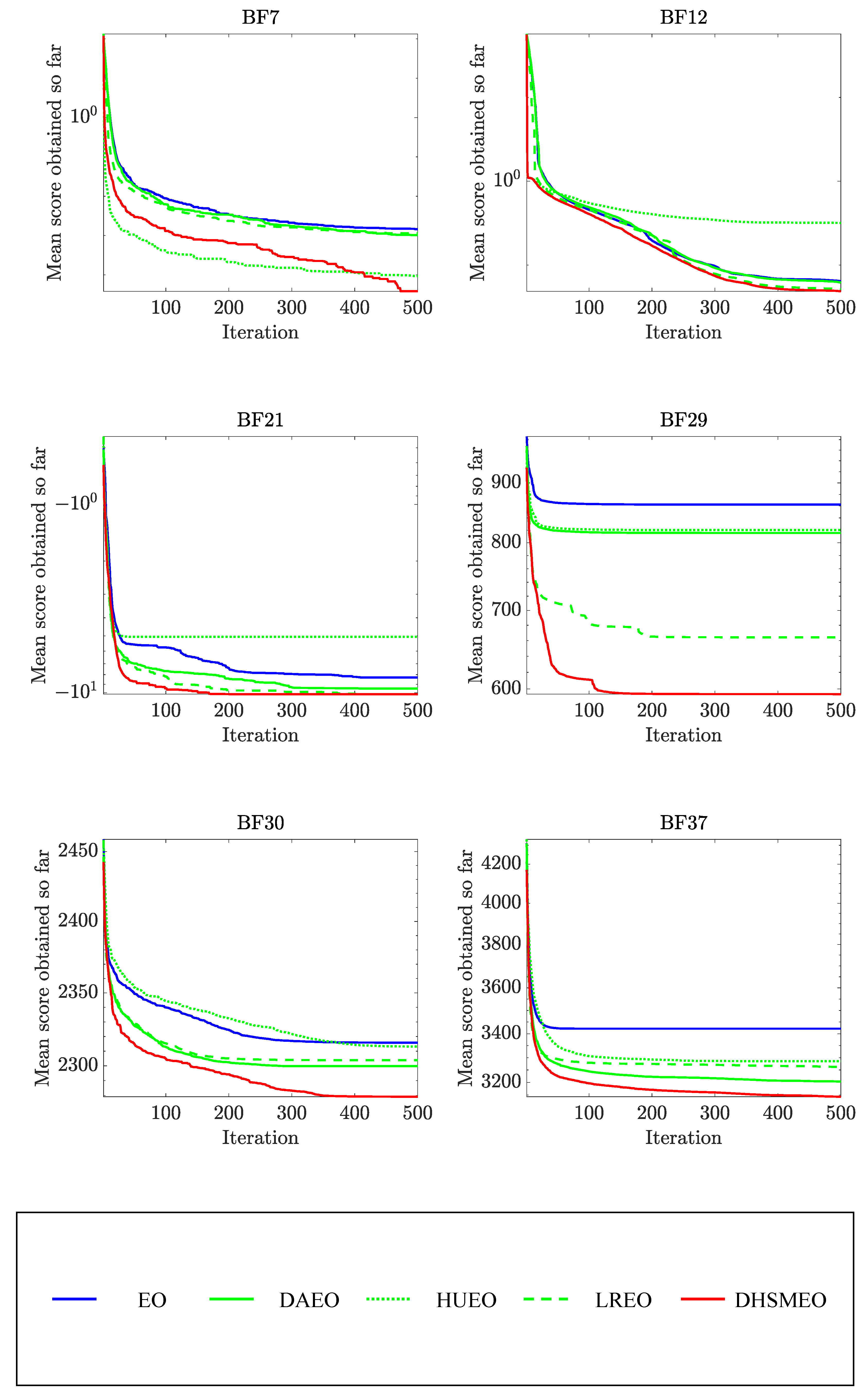
4.4. Impacts of Improvement Strategies on EO

DHSMEO aims to boost optimization capability by integrating the dynamic heterogeneous search-mutation structure, which consists of the dynamic dual-subpopulation adaptive grouping strategy, the heterogeneous hybrid search-based concentration-updating strategy, and the dynamic Levy mutation-based optimal equilibrium candidate-refining strategy. To evaluate the impacts of the above enhancement strategies within the constructed dynamic heterogeneous search-mutation structure over the EO, this subsection conducts the performance analysis over the standard EO, as well as four variants of EO (DAEO, HUEO, LREO, and DHSMEO) across the 39 typical benchmark functions. In this subsection, the DAEO represents an EO variant that incorporates the dynamic dual-subpopulation adaptive grouping strategy. HUEO denotes an EO variant that introduces the heterogeneous hybrid search-based concentration-updating strategy. LREO refers to an EO variant that combines the dynamic Levy mutation-based optimal equilibrium candidate-refining strategy. DHSMEO represents the EO variant proposed in this paper, which is obtained by simultaneously integrating all three improvement strategies to form a dynamic heterogeneous search-mutation structure.

A total of 30 independent tests are conducted for the standard EO and its four variants over each benchmark function.

Table 5. Test results of different improvement strategies in unimodal benchmark functions.

	Problem		EO	DAEO	HUEO	LREO	DHSMEO
Unimodal	BF1	Avg	$4.572\times {10}^{-41}$	$4.291\times {10}^{-53}$	$0.000\times {10}^0$	$1.364\times {10}^{-167}$	$\mathbf{0.000}\times {\mathbf{10}}^{\mathbf{0}}$
		Std	$4.015\times {10}^{-41}$	$5.057\times {10}^{-53}$	$0.000\times {10}^0$	$0.000\times {10}^0$	$0.000\times {10}^0$
	BF2	Avg	$9.844\times {10}^{-24}$	$2.858\times {10}^{-31}$	$0.000\times {10}^0$	$3.752\times {10}^{-87}$	$\mathbf{0.000}\times {\mathbf{10}}^{\mathbf{0}}$
		Std	$9.957\times {10}^{-24}$	$2.189\times {10}^{-31}$	$0.000\times {10}^0$	$1.559\times {10}^{-86}$	$0.000\times {10}^0$
	BF3	Avg	$9.900\times {10}^{-9}$	$1.390\times {10}^{-14}$	$0.000\times {10}^0$	$1.774\times {10}^{-145}$	$\mathbf{0.000}\times {\mathbf{10}}^{\mathbf{0}}$
		Std	$3.708\times {10}^{-8}$	$1.969\times {10}^{-14}$	$0.000\times {10}^0$	$9.196\times {10}^{-145}$	$0.000\times {10}^0$
	BF4	Avg	$2.767\times {10}^{-10}$	$3.528\times {10}^{-12}$	$0.000\times {10}^0$	$1.781\times {10}^{-76}$	$\mathbf{0.000}\times {\mathbf{10}}^{\mathbf{0}}$
		Std	$2.546\times {10}^{-10}$	$3.351\times {10}^{-12}$	$0.000\times {10}^0$	$9.686\times {10}^{-76}$	$0.000\times {10}^0$
	BF5	Avg	$2.544\times {10}^1$	$2.511\times {10}^1$	$2.600\times {10}^1$	$2.512\times {10}^1$	$\mathbf{2.507}\times {\mathbf{10}}^{\mathbf{1}}$
		Std	$1.159\times {10}^{-1}$	$6.215\times {10}^{-2}$	$1.154\times {10}^{-1}$	$6.928\times {10}^{-2}$	$7.996\times {10}^{-2}$
	BF6	Avg	$1.008\times {10}^{-5}$	$7.051\times {10}^{-6}$	$1.400\times {10}^{-1}$	$5.142\times {10}^{-6}$	$\mathbf{4.816}\times {\mathbf{10}}^{-\mathbf{6}}$
		Std	$3.830\times {10}^{-6}$	$2.498\times {10}^{-6}$	$1.482\times {10}^{-1}$	$1.753\times {10}^{-6}$	$1.465\times {10}^{-6}$
	BF7	Avg	$1.452\times {10}^{-3}$	$1.020\times {10}^{-3}$	$9.312\times {10}^{-5}$	$1.142\times {10}^{-3}$	$\mathbf{3.824}\times {\mathbf{10}}^{-\mathbf{5}}$
		Std	$4.282\times {10}^{-4}$	$4.532\times {10}^{-4}$	$4.308\times {10}^{-5}$	$5.688\times {10}^{-4}$	$2.492\times {10}^{-5}$

,

Table 6. Test results of different improvement strategies in multimodal benchmark functions with high dimension.

	Problem		EO	DAEO	HUEO	LREO	DHSMEO
Multimodal	BF8	Avg	−$8.650\times {10}^3$	−$9.052\times {10}^3$	−$8.764\times {10}^3$	−$8.962\times {10}^3$	−$\mathbf{9.801}\times {\mathbf{10}}^{\mathbf{3}}$
(High		Std	$4.107\times {10}^2$	$2.807\times {10}^2$	$3.918\times {10}^2$	$3.111\times {10}^2$	$3.772\times {10}^2$
dimension)	BF9	Avg	$0.000\times {10}^0$	$0.000\times {10}^0$	$0.000\times {10}^0$	$0.000\times {10}^0$	$\mathbf{0.000}\times {\mathbf{10}}^{\mathbf{0}}$
		Std	$0.000\times {10}^0$	$0.000\times {10}^0$	$0.000\times {10}^0$	$0.000\times {10}^0$	$0.000\times {10}^0$
	BF10	Avg	$9.652\times {10}^{-15}$	$6.099\times {10}^{-15}$	$8.882\times {10}^{-16}$	$8.882\times {10}^{-16}$	$\mathbf{8.882}\times {\mathbf{10}}^{-\mathbf{16}}$
		Std	$3.057\times {10}^{-15}$	$1.803\times {10}^{-15}$	$0.000\times {10}^0$	$0.000\times {10}^0$	$0.000\times {10}^0$
	BF11	Avg	$0.000\times {10}^0$	$0.000\times {10}^0$	$0.000\times {10}^0$	$0.000\times {10}^0$	$\mathbf{0.000}\times {\mathbf{10}}^{\mathbf{0}}$
		Std	$0.000\times {10}^0$	$0.000\times {10}^0$	$0.000\times {10}^0$	$0.000\times {10}^0$	$0.000\times {10}^0$
	BF12	Avg	$1.072\times {10}^{-6}$	$8.841\times {10}^{-7}$	$3.264\times {10}^{-3}$	$3.465\times {10}^{-7}$	$\mathbf{2.716}\times {\mathbf{10}}^{-\mathbf{7}}$
		Std	$8.011\times {10}^{-7}$	$3.294\times {10}^{-7}$	$3.504\times {10}^{-3}$	$1.453\times {10}^{-7}$	$6.933\times {10}^{-8}$
	BF13	Avg	$4.834\times {10}^{-2}$	$\mathbf{3.839}\times {\mathbf{10}}^{-\mathbf{2}}$	$2.139\times {10}^0$	$1.227\times {10}^{-1}$	$5.501\times {10}^{-1}$
		Std	$4.640\times {10}^{-2}$	$4.672\times {10}^{-2}$	$1.458\times {10}^{-1}$	$1.765\times {10}^{-1}$	$2.201\times {10}^{-1}$

,

Table 7. Test results of different improvement strategies in multimodal benchmark functions with fixed dimension.

	Problem		EO	DAEO	HUEO	LREO	DHSMEO
Multimodal	BF14	Avg	$9.980\times {10}^{-1}$	$9.980\times {10}^{-1}$	$9.980\times {10}^{-1}$	$9.980\times {10}^{-1}$	$\mathbf{9.980}\times {\mathbf{10}}^{-\mathbf{1}}$
(Fixed-		Std	$2.102\times {10}^{-16}$	$2.369\times {10}^{-16}$	$1.649\times {10}^{-16}$	$1.749\times {10}^{-16}$	$0.000\times {10}^0$
dimension)	BF15	Avg	$8.438\times {10}^{-3}$	$1.811\times {10}^{-3}$	$3.436\times {10}^{-4}$	$3.920\times {10}^{-3}$	$\mathbf{3.080}\times {\mathbf{10}}^{-\mathbf{4}}$
		Std	$9.907\times {10}^{-3}$	$5.057\times {10}^{-3}$	$5.582\times {10}^{-5}$	$7.492\times {10}^{-3}$	$5.783\times {10}^{-7}$
	BF16	Avg	−$1.032\times {10}^0$	−$1.032\times {10}^0$	−$1.032\times {10}^0$	−$1.032\times {10}^0$	−$\mathbf{1.032}\times {\mathbf{10}}^{\mathbf{0}}$
		Std	$5.758\times {10}^{-16}$	$5.296\times {10}^{-16}$	$5.216\times {10}^{-16}$	$5.133\times {10}^{-16}$	$6.775\times {10}^{-16}$
	BF17	Avg	$3.979\times {10}^{-1}$	$3.979\times {10}^{-1}$	$3.979\times {10}^{-1}$	$3.979\times {10}^{-1}$	$\mathbf{3.979}\times {\mathbf{10}}^{-\mathbf{1}}$
		Std	$0.000\times {10}^0$	$0.000\times {10}^0$	$0.000\times {10}^0$	$0.000\times {10}^0$	$0.000\times {10}^0$
	BF18	Avg	$3.000\times {10}^0$	$3.000\times {10}^0$	$3.000\times {10}^0$	$3.000\times {10}^0$	$\mathbf{3.000}\times {\mathbf{10}}^{\mathbf{0}}$
		Std	$1.259\times {10}^{-15}$	$1.291\times {10}^{-15}$	$1.286\times {10}^{-15}$	$1.738\times {10}^{-15}$	$2.171\times {10}^{-15}$
	BF19	Avg	−$3.863\times {10}^0$	−$3.863\times {10}^0$	−$3.863\times {10}^0$	−$3.863\times {10}^0$	−$\mathbf{3.863}\times {\mathbf{10}}^{\mathbf{0}}$
		Std	$2.464\times {10}^{-15}$	$2.479\times {10}^{-15}$	$2.258\times {10}^{-15}$	$2.324\times {10}^{-15}$	$2.710\times {10}^{-15}$
	BF20	Avg	−$3.231\times {10}^0$	−$3.306\times {10}^0$	−$3.255\times {10}^0$	−$3.286\times {10}^0$	−$\mathbf{3.322}\times {\mathbf{10}}^{\mathbf{0}}$
		Std	$5.126\times {10}^{-2}$	$4.111\times {10}^{-2}$	$5.992\times {10}^{-2}$	$5.542\times {10}^{-2}$	$1.355\times {10}^{-15}$
	BF21	Avg	−$8.287\times {10}^0$	−$9.478\times {10}^0$	−$5.055\times {10}^0$	−$1.015\times {10}^1$	−$\mathbf{1.015}\times {\mathbf{10}}^{\mathbf{1}}$
		Std	$2.495\times {10}^0$	$1.751\times {10}^0$	$1.565\times {10}^{-15}$	$6.218\times {10}^{-6}$	$5.637\times {10}^{-15}$
	BF22	Avg	−$9.694\times {10}^0$	−$9.874\times {10}^0$	−$5.619\times {10}^0$	−$1.040\times {10}^1$	−$\mathbf{1.040}\times {\mathbf{10}}^{\mathbf{1}}$
		Std	$1.838\times {10}^0$	$1.613\times {10}^0$	$1.622\times {10}^0$	$4.850\times {10}^{-5}$	$5.713\times {10}^{-16}$
	BF23	Avg	−$9.455\times {10}^0$	−$1.027\times {10}^1$	−$6.304\times {10}^0$	−$1.054\times {10}^1$	−$\mathbf{1.054}\times {\mathbf{10}}^{\mathbf{1}}$
		Std	$2.200\times {10}^0$	$1.482\times {10}^0$	$2.397\times {10}^0$	$4.205\times {10}^{-5}$	$2.618\times {10}^{-15}$

,

Table 8. Test results of different improvement strategies in composition benchmark functions.

	Problem		EO	DAEO	HUEO	LREO	DHSMEO
Composition	BF24	Avg	$6.000\times {10}^1$	$3.000\times {10}^1$	$3.333\times {10}^1$	$1.667\times {10}^1$	$\mathbf{6.247}\times {\mathbf{10}}^{-\mathbf{17}}$
		Std	$6.215\times {10}^1$	$4.661\times {10}^1$	$4.795\times {10}^1$	$3.790\times {10}^1$	$7.290\times {10}^{-17}$
	BF25	Avg	$1.303\times {10}^2$	$2.985\times {10}^1$	$4.489\times {10}^1$	$6.704\times {10}^1$	$\mathbf{2.263}\times {\mathbf{10}}^{\mathbf{0}}$
		Std	$5.632\times {10}^1$	$3.969\times {10}^1$	$5.568\times {10}^1$	$6.160\times {10}^1$	$1.889\times {10}^0$
	BF26	Avg	$1.721\times {10}^2$	$1.648\times {10}^2$	$2.662\times {10}^2$	$1.572\times {10}^2$	$\mathbf{1.202}\times {\mathbf{10}}^{\mathbf{2}}$
		Std	$2.824\times {10}^1$	$3.182\times {10}^1$	$2.581\times {10}^2$	$2.039\times {10}^1$	$9.365\times {10}^0$
	BF27	Avg	$4.093\times {10}^2$	$3.156\times {10}^2$	$3.949\times {10}^2$	$3.117\times {10}^2$	$\mathbf{2.879}\times {\mathbf{10}}^{\mathbf{2}}$
		Std	$1.231\times {10}^2$	$1.485\times {10}^1$	$1.100\times {10}^2$	$1.236\times {10}^1$	$9.977\times {10}^0$
	BF28	Avg	$6.517\times {10}^1$	$6.317\times {10}^0$	$3.631\times {10}^1$	$3.376\times {10}^1$	$\mathbf{1.433}\times {\mathbf{10}}^{\mathbf{0}}$
		Std	$4.733\times {10}^1$	$2.507\times {10}^0$	$4.665\times {10}^1$	$4.459\times {10}^1$	$8.503\times {10}^{-1}$
	BF29	Avg	$8.623\times {10}^2$	$8.155\times {10}^2$	$8.201\times {10}^2$	$6.641\times {10}^2$	$\mathbf{5.940}\times {\mathbf{10}}^{\mathbf{2}}$
		Std	$1.227\times {10}^2$	$1.703\times {10}^2$	$1.625\times {10}^2$	$1.918\times {10}^2$	$1.600\times {10}^2$
	BF30	Avg	$2.316\times {10}^3$	$2.300\times {10}^3$	$2.313\times {10}^3$	$2.304\times {10}^3$	$\mathbf{2.279}\times {\mathbf{10}}^{\mathbf{3}}$
		Std	$4.620\times {10}^0$	$3.927\times {10}^1$	$3.003\times {10}^0$	$3.454\times {10}^1$	$4.745\times {10}^1$
	BF31	Avg	$2.301\times {10}^3$	$2.295\times {10}^3$	$2.301\times {10}^3$	$2.299\times {10}^3$	$\mathbf{2.289}\times {\mathbf{10}}^{\mathbf{3}}$
		Std	$4.319\times {10}^{-1}$	$1.982\times {10}^1$	$2.518\times {10}^{-1}$	$8.864\times {10}^0$	$2.931\times {10}^1$
	BF32	Avg	$2.619\times {10}^3$	$2.618\times {10}^3$	$2.615\times {10}^3$	$2.616\times {10}^3$	$\mathbf{2.610}\times {\mathbf{10}}^{\mathbf{3}}$
		Std	$4.387\times {10}^0$	$4.205\times {10}^0$	$3.428\times {10}^0$	$4.031\times {10}^0$	$2.576\times {10}^0$
	BF33	Avg	$2.749\times {10}^3$	$2.729\times {10}^3$	$2.739\times {10}^3$	$2.735\times {10}^3$	$\mathbf{2.721}\times {\mathbf{10}}^{\mathbf{3}}$
		Std	$7.531\times {10}^0$	$6.245\times {10}^1$	$3.744\times {10}^0$	$4.459\times {10}^1$	$6.004\times {10}^1$
	BF34	Avg	$2.946\times {10}^3$	$2.911\times {10}^3$	$2.916\times {10}^3$	$2.913\times {10}^3$	$\mathbf{2.899}\times {\mathbf{10}}^{\mathbf{3}}$
		Std	$1.674\times {10}^0$	$2.044\times {10}^1$	$2.185\times {10}^1$	$2.089\times {10}^1$	$7.620\times {10}^{-1}$
	BF35	Avg	$3.041\times {10}^3$	$2.905\times {10}^3$	$2.886\times {10}^3$	$2.916\times {10}^3$	$\mathbf{2.843}\times {\mathbf{10}}^{\mathbf{3}}$
		Std	$2.723\times {10}^2$	$9.689\times {10}^1$	$5.966\times {10}^1$	$5.016\times {10}^1$	$5.040\times {10}^1$
	BF36	Avg	$3.097\times {10}^3$	$3.092\times {10}^3$	$3.094\times {10}^3$	$3.093\times {10}^3$	$\mathbf{3.090}\times {\mathbf{10}}^{\mathbf{3}}$
		Std	$9.015\times {10}^0$	$1.882\times {10}^0$	$1.756\times {10}^0$	$1.824\times {10}^0$	$5.358\times {10}^{-1}$
	BF37	Avg	$3.422\times {10}^3$	$3.204\times {10}^3$	$3.285\times {10}^3$	$3.262\times {10}^3$	$\mathbf{3.144}\times {\mathbf{10}}^{\mathbf{3}}$
		Std	$5.882\times {10}^1$	$1.288\times {10}^2$	$1.032\times {10}^2$	$1.357\times {10}^2$	$3.248\times {10}^1$
	BF38	Avg	$3.188\times {10}^3$	$3.181\times {10}^3$	$3.182\times {10}^3$	$3.183\times {10}^3$	$\mathbf{3.153}\times {\mathbf{10}}^{\mathbf{3}}$
		Std	$2.246\times {10}^1$	$2.128\times {10}^1$	$1.409\times {10}^1$	$2.095\times {10}^1$	$8.356\times {10}^0$
	BF39	Avg	$3.532\times {10}^5$	$1.381\times {10}^4$	$2.389\times {10}^5$	$7.332\times {10}^4$	$\mathbf{1.174}\times {\mathbf{10}}^{\mathbf{4}}$
		Std	$4.494\times {10}^5$	$7.249\times {10}^3$	$3.418\times {10}^5$	$2.036\times {10}^5$	$4.459\times {10}^3$

and

Table 9. Non-parametric test results of different improvement strategies in 39 typical benchmark functions.

		EO	DAEO	HUEO	LREO	DHSMEO
Friedman mean rank		4.436	2.769	3.462	2.872	1.462
Final rank		5	2	4	3	1
1/0/−1		32/6/1	32/6/1	28/11/0	31/7/1	∼

present the corresponding results for the Avg, the Std, the Wilcoxon signed-rank test, the and Friedman test. In Table 5, Table 6, Table 7, Table 8 and Table 9, the best results achieved across the 39 typical benchmark functions, along with their corresponding optimal algorithms, are emphasized in bold.

The comparative results from Table 5, Table 6, Table 7 and Table 8 show that EO, DAEO, HUEO, and LREO achieve the best results with 6, 7, 11, and 7 out of the 39 typical benchmark functions, respectively. In contrast, DHSMEO achieves the best performance in 38 of 39 benchmark functions and exhibits superior optimization performance compared to EO, DAEO, HUEO, and LREO in most cases. This result indicates that DHSMEO achieves the best performance through effectively integrating three improvement strategies to form a dynamic heterogeneous search-mutation structure. Table 9 further exhibits the corresponding results for Wilcoxon signed-rank test and Friedman test in the 39 typical benchmark functions. The Wilcoxon signed-rank test results, represented as ‘1/0/−1’, denote that DHSMEO excels EO, DAEO, HUEO, and LREO across 32, 32, 28, and 31 benchmark functions. This result demonstrates that DHSMEO exhibits significantly better performance than the standard EO and other EO variants in most circumstances. The Friedman test results, presented in terms of Friedman mean rank and final rank in Table 9, assess the overall optimization performance of different EO variants. According to the Friedman test results, HUEO obtains the fourth place in the final rank with a Friedman mean rank of 3.462. This result shows that the heterogeneous hybrid search-based concentration-updating strategy improves the performance of EO by enhancing search efficiency. LREO achieves a Friedman mean rank of 2.872, placing it in third place in the final rank. This result indicates that the dynamic Levy mutation-based optimal equilibrium candidate-refining strategy is more effective than the heterogeneous hybrid search-based concentration-updating strategy in improving the optimization performance of EO by strengthening the capability of escaping local optima. The Friedman analysis assigns DAEO a Friedman mean rank of 2.769, ranking its placement at the second place of the final rank. This results show that the dynamic dual-subpopulation adaptive grouping strategy plays a key role in improving the performance of EO by boosting population diversity. The EO attains a Friedman mean rank of 4.436, situating it at the lowest position in the final rank. This result further confirms that the three enhancement strategies successfully increase the search capability for the standard EO. Meanwhile, with an outstanding Friedman mean rank of 1.462, DHSMEO secures the top position among the EO variants in the final rank. This result suggests that DHSMEO presents the best overall performance among the EO variants by combining these three improvement strategies simultaneously to form the dynamic heterogeneous search-mutation structure. Additionally, the convergence curves of EO, DAEO, HUEO, LREO, and DHSMEO on six benchmark functions are depicted in Figure 2 to visually assess their convergence capability. In Figure 2, the y-axis represents the mean fitness value obtained over 30 independent tests, while the x-axis denotes the number of iterations. The convergence curves of various EO variants in Figure 2 demonstrate that DHSMEO performs superior convergence accuracy and convergence speed.

In summary, based on numerical experimental results and convergence curves, all three enhancement strategies assist in enhancing the optimization capability for the standard EO. And DHSMEO obtained by introducing these three strategies to form the dynamic heterogeneous search-mutation structure exhibits better capability than the standard EO and other EO variants. Therefore, DHSMEO is regarded as the ultimate effective variant of the standard EO, which will be compared with a collection of recently proposed algorithms in the next subsection to further validate its superiority.

4.5. Comparative Test of DHSMEO and Other Algorithms

The effectiveness of the dynamic dual-subpopulation adaptive grouping strategy, the heterogeneous hybrid search-based concentration-updating strategy, and the dynamic Levy mutation-based optimal equilibrium candidate-refining strategy within the dynamic heterogeneous search-mutation structure is verified in the previous subsection. And DHSMEO is identified as the ultimate effective variant of the standard EO. In this subsection, DHSMEO is compared with a collection of recently proposed algorithms (EO [13], RSA [11], SMA [7], HGS [9], DMMAEO [21], DEEO [32], HRSA [33], ESMA [34], and AOAHGS [35]) on the 39 typical benchmark functions to further analyze the superiority of DHSMEO. The above comparative algorithms involve three diverse types: recently well-established algorithms (EO, RSA, SMA, and HGS), EO-based variants (DMMAEO and DEEO), and other enhanced algorithms (HRSA, ESMA, and AOAHGS). The parameter values of other algorithms within the comparative analysis are configured in accordance with corresponding source references.

Table 10. Test results for DHSMEO and compared algorithms in unimodal benchmark functions.

	Problem		EO	RSA	SMA	HGS	DMMAEO
Unimodal	BF1	Avg	$4.572\times {10}^{-41}$	$0.000\times {10}^0$	$0.000\times {10}^0$	$2.548\times {10}^{-156}$	$0.000\times {10}^0$
		Std	$4.015\times {10}^{-41}$	$0.000\times {10}^0$	$0.000\times {10}^0$	$1.390\times {10}^{-155}$	$0.000\times {10}^0$
	BF2	Avg	$9.844\times {10}^{-24}$	$0.000\times {10}^0$	$6.661\times {10}^{-168}$	$9.350\times {10}^{-88}$	$3.361\times {10}^{-308}$
		Std	$9.957\times {10}^{-24}$	$0.000\times {10}^0$	$0.000\times {10}^0$	$2.850\times {10}^{-87}$	$0.000\times {10}^0$
	BF3	Avg	$9.900\times {10}^{-9}$	$0.000\times {10}^0$	$0.000\times {10}^0$	$7.709\times {10}^{-69}$	$0.000\times {10}^0$
		Std	$3.708\times {10}^{-8}$	$0.000\times {10}^0$	$0.000\times {10}^0$	$3.435\times {10}^{-68}$	$0.000\times {10}^0$
	BF4	Avg	$2.767\times {10}^{-10}$	$0.000\times {10}^0$	$3.823\times {10}^{-166}$	$4.178\times {10}^{-67}$	$6.520\times {10}^{-306}$
		Std	$2.546\times {10}^{-10}$	$0.000\times {10}^0$	$0.000\times {10}^0$	$1.928\times {10}^{-66}$	$0.000\times {10}^0$
	BF5	Avg	$2.544\times {10}^1$	$1.789\times {10}^1$	$5.019\times {10}^0$	$2.268\times {10}^1$	$2.472\times {10}^1$
		Std	$1.159\times {10}^{-1}$	$1.402\times {10}^1$	$8.022\times {10}^0$	$7.682\times {10}^0$	$1.368\times {10}^{-1}$
	BF6	Avg	$1.008\times {10}^{-5}$	$7.126\times {10}^0$	$6.146\times {10}^{-3}$	$5.622\times {10}^{-6}$	$\mathbf{1.541}\times {\mathbf{10}}^{-\mathbf{6}}$
		Std	$3.830\times {10}^{-6}$	$1.288\times {10}^{-1}$	$1.718\times {10}^{-3}$	$4.135\times {10}^{-6}$	$7.254\times {10}^{-7}$
	BF7	Avg	$1.452\times {10}^{-3}$	$1.289\times {10}^{-4}$	$2.243\times {10}^{-4}$	$8.059\times {10}^{-4}$	$4.766\times {10}^{-5}$
		Std	$4.282\times {10}^{-4}$	$7.633\times {10}^{-5}$	$1.223\times {10}^{-4}$	$7.635\times {10}^{-4}$	$2.450\times {10}^{-5}$
	Problem		DEEO	HRSA	ESMA	AOAHGS	DHSMEO
	BF1	Avg	$9.675\times {10}^{-22}$	$0.000\times {10}^0$	$0.000\times {10}^0$	$0.000\times {10}^0$	$\mathbf{0.000}\times {\mathbf{10}}^{\mathbf{0}}$
		Std	$6.645\times {10}^{-22}$	$0.000\times {10}^0$	$0.000\times {10}^0$	$0.000\times {10}^0$	$0.000\times {10}^0$
	BF2	Avg	$2.458\times {10}^{-13}$	$0.000\times {10}^0$	$4.209\times {10}^{-236}$	$0.000\times {10}^0$	$\mathbf{0.000}\times {\mathbf{10}}^{\mathbf{0}}$
		Std	$8.407\times {10}^{-14}$	$0.000\times {10}^0$	$0.000\times {10}^0$	$0.000\times {10}^0$	$0.000\times {10}^0$
	BF3	Avg	$4.145\times {10}^{-3}$	$0.000\times {10}^0$	$0.000\times {10}^0$	$4.010\times {10}^{-135}$	$\mathbf{0.000}\times {\mathbf{10}}^{\mathbf{0}}$
		Std	$4.934\times {10}^{-3}$	$0.000\times {10}^0$	$0.000\times {10}^0$	$1.512\times {10}^{-134}$	$0.000\times {10}^0$
	BF4	Avg	$2.920\times {10}^{-5}$	$0.000\times {10}^0$	$6.917\times {10}^{-323}$	$1.241\times {10}^{-66}$	$\mathbf{0.000}\times {\mathbf{10}}^{\mathbf{0}}$
		Std	$1.486\times {10}^{-5}$	$0.000\times {10}^0$	$0.000\times {10}^0$	$2.928\times {10}^{-66}$	$0.000\times {10}^0$
	BF5	Avg	$2.555\times {10}^1$	$2.896\times {10}^1$	$\mathbf{4.277}\times {\mathbf{10}}^{-\mathbf{1}}$	$2.282\times {10}^1$	$2.507\times {10}^1$
		Std	$1.631\times {10}^{-1}$	$6.764\times {10}^{-2}$	$3.179\times {10}^{-1}$	$1.035\times {10}^1$	$7.996\times {10}^{-2}$
	BF6	Avg	$1.592\times {10}^{-5}$	$4.328\times {10}^0$	$1.526\times {10}^{-3}$	$1.372\times {10}^{-4}$	$4.816\times {10}^{-6}$
		Std	$7.366\times {10}^{-6}$	$1.385\times {10}^0$	$5.754\times {10}^{-4}$	$1.453\times {10}^{-4}$	$1.465\times {10}^{-6}$
	BF7	Avg	$2.507\times {10}^{-3}$	$1.165\times {10}^{-4}$	$7.383\times {10}^{-5}$	$5.294\times {10}^{-5}$	$\mathbf{3.824}\times {\mathbf{10}}^{-\mathbf{5}}$
		Std	$6.013\times {10}^{-4}$	$8.014\times {10}^{-5}$	$4.497\times {10}^{-5}$	$2.400\times {10}^{-5}$	$2.492\times {10}^{-5}$

,

Table 11. Test results for DHSMEO and compared algorithms in multimodal benchmark functions with high dimension.

	Problem		EO	RSA	SMA	HGS	DMMAEO
Multimodal	BF8	Avg	−$8.650\times {10}^3$	−$5.420\times {10}^3$	−$1.257\times {10}^4$	−$1.257\times {10}^4$	−$9.263\times {10}^3$
(High		Std	$4.107\times {10}^2$	$1.115\times {10}^2$	$2.367\times {10}^{-1}$	$9.574\times {10}^0$	$7.004\times {10}^2$
dimension)	BF9	Avg	$0.000\times {10}^0$	$0.000\times {10}^0$	$0.000\times {10}^0$	$0.000\times {10}^0$	$0.000\times {10}^0$
		Std	$0.000\times {10}^0$	$0.000\times {10}^0$	$0.000\times {10}^0$	$0.000\times {10}^0$	$0.000\times {10}^0$
	BF10	Avg	$9.652\times {10}^{-15}$	$8.882\times {10}^{-16}$	$8.882\times {10}^{-16}$	$8.882\times {10}^{-16}$	$8.882\times {10}^{-16}$
		Std	$3.057\times {10}^{-15}$	$0.000\times {10}^0$	$0.000\times {10}^0$	$0.000\times {10}^0$	$0.000\times {10}^0$
	BF11	Avg	$0.000\times {10}^0$	$0.000\times {10}^0$	$0.000\times {10}^0$	$0.000\times {10}^0$	$0.000\times {10}^0$
		Std	$0.000\times {10}^0$	$0.000\times {10}^0$	$0.000\times {10}^0$	$0.000\times {10}^0$	$0.000\times {10}^0$
	BF12	Avg	$1.072\times {10}^{-6}$	$1.451\times {10}^0$	$4.355\times {10}^{-3}$	$2.183\times {10}^{-4}$	$3.620\times {10}^{-7}$
		Std	$8.011\times {10}^{-7}$	$1.969\times {10}^{-1}$	$3.480\times {10}^{-3}$	$1.195\times {10}^{-3}$	$2.479\times {10}^{-7}$
	BF13	Avg	$4.834\times {10}^{-2}$	$1.626\times {10}^{-1}$	$6.749\times {10}^{-3}$	$\mathbf{1.652}\times {\mathbf{10}}^{-\mathbf{6}}$	$1.123\times {10}^0$
		Std	$4.640\times {10}^{-2}$	$4.819\times {10}^{-1}$	$3.943\times {10}^{-3}$	$7.887\times {10}^{-7}$	$4.793\times {10}^{-1}$
	Problem		DEEO	HRSA	ESMA	AOAHGS	DHSMEO
	BF8	Avg	−$7.186\times {10}^3$	−$9.323\times {10}^3$	−$\mathbf{1.257}\times {\mathbf{10}}^{\mathbf{4}}$	−$1.256\times {10}^4$	−$9.801\times {10}^3$
		Std	$9.129\times {10}^2$	$8.374\times {10}^2$	$7.374\times {10}^{-2}$	$8.745\times {10}^0$	$3.772\times {10}^2$
	BF9	Avg	$0.000\times {10}^0$	$0.000\times {10}^0$	$0.000\times {10}^0$	$0.000\times {10}^0$	$\mathbf{0.000}\times {\mathbf{10}}^{\mathbf{0}}$
		Std	$0.000\times {10}^0$	$0.000\times {10}^0$	$0.000\times {10}^0$	$0.000\times {10}^0$	$0.000\times {10}^0$
	BF10	Avg	$5.123\times {10}^{-12}$	$8.882\times {10}^{-16}$	$8.882\times {10}^{-16}$	$8.882\times {10}^{-16}$	$\mathbf{8.882}\times {\mathbf{10}}^{-\mathbf{16}}$
		Std	$1.464\times {10}^{-12}$	$0.000\times {10}^0$	$0.000\times {10}^0$	$0.000\times {10}^0$	$0.000\times {10}^0$
	BF11	Avg	$0.000\times {10}^0$	$0.000\times {10}^0$	$0.000\times {10}^0$	$0.000\times {10}^0$	$\mathbf{0.000}\times {\mathbf{10}}^{\mathbf{0}}$
		Std	$0.000\times {10}^0$	$0.000\times {10}^0$	$0.000\times {10}^0$	$0.000\times {10}^0$	$0.000\times {10}^0$
	BF12	Avg	$1.012\times {10}^{-6}$	$3.847\times {10}^{-1}$	$9.178\times {10}^{-4}$	$1.300\times {10}^{-5}$	$\mathbf{2.716}\times {\mathbf{10}}^{-\mathbf{7}}$
		Std	$4.465\times {10}^{-7}$	$2.894\times {10}^{-1}$	$7.251\times {10}^{-4}$	$1.587\times {10}^{-5}$	$6.933\times {10}^{-8}$
	BF13	Avg	$3.715\times {10}^{-3}$	$2.274\times {10}^0$	$1.273\times {10}^{-3}$	$2.193\times {10}^{-4}$	$5.501\times {10}^{-1}$
		Std	$5.248\times {10}^{-3}$	$9.344\times {10}^{-1}$	$6.014\times {10}^{-4}$	$2.839\times {10}^{-4}$	$2.201\times {10}^{-1}$

,

Table 12. Test results for DHSMEO and compared algorithms in multimodal benchmark functions with fixed dimension.

	Problem		EO	RSA	SMA	HGS	DMMAEO
Multimodal	BF14	Avg	$9.980\times {10}^{-1}$	$4.388\times {10}^0$	$9.980\times {10}^{-1}$	$1.649\times {10}^0$	$9.980\times {10}^{-1}$
(Fixed-		Std	$2.102\times {10}^{-16}$	$2.478\times {10}^0$	$2.778\times {10}^{-13}$	$2.478\times {10}^0$	$0.000\times {10}^0$
dimension)	BF15	Avg	$8.438\times {10}^{-3}$	$1.437\times {10}^{-3}$	$6.404\times {10}^{-4}$	$7.562\times {10}^{-4}$	$3.082\times {10}^{-4}$
		Std	$9.907\times {10}^{-3}$	$3.653\times {10}^{-4}$	$1.557\times {10}^{-4}$	$1.171\times {10}^{-4}$	$1.392\times {10}^{-6}$
	BF16	Avg	−$1.032\times {10}^0$	−$1.031\times {10}^0$	−$1.032\times {10}^0$	−$1.032\times {10}^0$	−$1.032\times {10}^0$
		Std	$5.758\times {10}^{-16}$	$5.912\times {10}^{-4}$	$4.390\times {10}^{-10}$	$6.649\times {10}^{-16}$	$6.775\times {10}^{-16}$
	BF17	Avg	$3.979\times {10}^{-1}$	$4.181\times {10}^{-1}$	$3.979\times {10}^{-1}$	$3.979\times {10}^{-1}$	$3.979\times {10}^{-1}$
		Std	$0.000\times {10}^0$	$1.487\times {10}^{-2}$	$1.260\times {10}^{-8}$	$0.000\times {10}^0$	$0.000\times {10}^0$
	BF18	Avg	$3.000\times {10}^0$	$3.000\times {10}^0$	$3.000\times {10}^0$	$3.000\times {10}^0$	$3.000\times {10}^0$
		Std	$1.259\times {10}^{-15}$	$4.144\times {10}^{-4}$	$2.345\times {10}^{-10}$	$1.932\times {10}^{-15}$	$1.688\times {10}^{-15}$
	BF19	Avg	−$3.863\times {10}^0$	−$3.799\times {10}^0$	−$3.863\times {10}^0$	−$3.863\times {10}^0$	−$3.863\times {10}^0$
		Std	$2.464\times {10}^{-15}$	$3.499\times {10}^{-2}$	$1.519\times {10}^{-7}$	$2.710\times {10}^{-15}$	$2.710\times {10}^{-15}$
	BF20	Avg	−$3.231\times {10}^0$	−$2.611\times {10}^0$	−$3.207\times {10}^0$	−$3.246\times {10}^0$	−$3.322\times {10}^0$
		Std	$5.126\times {10}^{-2}$	$2.646\times {10}^{-1}$	$2.176\times {10}^{-2}$	$6.493\times {10}^{-2}$	$1.424\times {10}^{-15}$
	BF21	Avg	−$8.287\times {10}^0$	−$5.055\times {10}^0$	−$1.015\times {10}^1$	−$9.643\times {10}^0$	−$1.015\times {10}^1$
		Std	$2.495\times {10}^0$	$1.322\times {10}^{-7}$	$1.542\times {10}^{-4}$	$1.556\times {10}^0$	$6.643\times {10}^{-6}$
	BF22	Avg	−$9.694\times {10}^0$	−$5.088\times {10}^0$	−$1.040\times {10}^1$	−$1.023\times {10}^1$	−$1.040\times {10}^1$
		Std	$1.838\times {10}^0$	$4.401\times {10}^{-7}$	$1.331\times {10}^{-4}$	$9.704\times {10}^{-1}$	$4.211\times {10}^{-6}$
	BF23	Avg	−$9.455\times {10}^0$	−$5.128\times {10}^0$	−$1.054\times {10}^1$	−$9.996\times {10}^0$	−$1.054\times {10}^1$
		Std	$2.200\times {10}^0$	$9.763\times {10}^{-7}$	$9.975\times {10}^{-5}$	$1.650\times {10}^0$	$6.669\times {10}^{-8}$
	Problem		DEEO	HRSA	ESMA	AOAHGS	DHSMEO
	BF14	Avg	$9.980\times {10}^{-1}$	$2.177\times {10}^0$	$9.980\times {10}^{-1}$	$2.366\times {10}^0$	$\mathbf{9.980}\times {\mathbf{10}}^{-\mathbf{1}}$
		Std	$0.000\times {10}^0$	$8.259\times {10}^{-1}$	$6.438\times {10}^{-14}$	$3.369\times {10}^0$	$0.000\times {10}^0$
	BF15	Avg	$\mathbf{3.075}\times {\mathbf{10}}^{-\mathbf{4}}$	$5.639\times {10}^{-4}$	$4.262\times {10}^{-4}$	$3.415\times {10}^{-4}$	$3.080\times {10}^{-4}$
		Std	$6.066\times {10}^{-12}$	$1.199\times {10}^{-4}$	$7.580\times {10}^{-5}$	$6.548\times {10}^{-5}$	$5.783\times {10}^{-7}$
	BF16	Avg	−$1.032\times {10}^0$	−$1.032\times {10}^0$	−$1.032\times {10}^0$	−$1.032\times {10}^0$	−$\mathbf{1.032}\times {\mathbf{10}}^{\mathbf{0}}$
		Std	$6.775\times {10}^{-16}$	$1.851\times {10}^{-5}$	$3.025\times {10}^{-10}$	$2.831\times {10}^{-12}$	$6.775\times {10}^{-16}$
	BF17	Avg	$3.979\times {10}^{-1}$	$3.979\times {10}^{-1}$	$3.979\times {10}^{-1}$	$3.979\times {10}^{-1}$	$\mathbf{3.979}\times {\mathbf{10}}^{-\mathbf{1}}$
		Std	$0.000\times {10}^0$	$2.236\times {10}^{-5}$	$9.901\times {10}^{-9}$	$7.139\times {10}^{-12}$	$0.000\times {10}^0$
	BF18	Avg	$3.000\times {10}^0$	$3.000\times {10}^0$	$3.000\times {10}^0$	$3.000\times {10}^0$	$\mathbf{3.000}\times {\mathbf{10}}^{\mathbf{0}}$
		Std	$1.355\times {10}^{-15}$	$2.194\times {10}^{-5}$	$5.649\times {10}^{-12}$	$3.687\times {10}^{-11}$	$2.171\times {10}^{-15}$
	BF19	Avg	−$3.863\times {10}^0$	−$3.858\times {10}^0$	−$3.863\times {10}^0$	−$3.863\times {10}^0$	−$\mathbf{3.863}\times {\mathbf{10}}^{\mathbf{0}}$
		Std	$2.710\times {10}^{-15}$	$3.617\times {10}^{-3}$	$9.552\times {10}^{-7}$	$6.199\times {10}^{-6}$	$2.710\times {10}^{-15}$
	BF20	Avg	−$3.231\times {10}^0$	−$3.126\times {10}^0$	−$3.282\times {10}^0$	−$3.290\times {10}^0$	−$\mathbf{3.322}\times {\mathbf{10}}^{\mathbf{0}}$
		Std	$5.115\times {10}^{-2}$	$7.798\times {10}^{-2}$	$5.702\times {10}^{-2}$	$4.717\times {10}^{-2}$	$1.355\times {10}^{-15}$
	BF21	Avg	−$1.015\times {10}^1$	−$1.002\times {10}^1$	−$1.015\times {10}^1$	−$1.015\times {10}^1$	−$\mathbf{1.015}\times {\mathbf{10}}^{\mathbf{1}}$
		Std	$6.328\times {10}^{-15}$	$7.315\times {10}^{-2}$	$1.063\times {10}^{-4}$	$9.680\times {10}^{-4}$	$5.637\times {10}^{-15}$
	BF22	Avg	−$1.040\times {10}^1$	−$1.022\times {10}^1$	−$1.040\times {10}^1$	−$1.040\times {10}^1$	−$\mathbf{1.040}\times {\mathbf{10}}^{\mathbf{1}}$
		Std	$0.000\times {10}^0$	$1.151\times {10}^{-1}$	$7.689\times {10}^{-5}$	$5.067\times {10}^{-3}$	$5.713\times {10}^{-16}$
	BF23	Avg	−$1.054\times {10}^1$	−$1.042\times {10}^1$	−$1.054\times {10}^1$	−$1.053\times {10}^1$	−$\mathbf{1.054}\times {\mathbf{10}}^{\mathbf{1}}$
		Std	$2.138\times {10}^{-15}$	$8.547\times {10}^{-2}$	$9.231\times {10}^{-5}$	$4.831\times {10}^{-3}$	$2.618\times {10}^{-15}$

,

Table 13. Test results for DHSMEO and compared algorithms in composition benchmark functions.

	Problem		EO	RSA	SMA	HGS	DMMAEO
Composition	BF24	Avg	$6.000\times {10}^1$	$3.700\times {10}^2$	$7.334\times {10}^1$	$1.433\times {10}^2$	$2.825\times {10}^{-7}$
		Std	$6.215\times {10}^1$	$6.903\times {10}^1$	$7.397\times {10}^1$	$5.683\times {10}^1$	$1.547\times {10}^{-6}$
	BF25	Avg	$1.303\times {10}^2$	$4.059\times {10}^2$	$2.890\times {10}^1$	$1.598\times {10}^2$	$3.490\times {10}^1$
		Std	$5.632\times {10}^1$	$5.751\times {10}^1$	$9.120\times {10}^0$	$7.163\times {10}^1$	$4.469\times {10}^1$
	BF26	Avg	$1.721\times {10}^2$	$8.876\times {10}^2$	$1.914\times {10}^2$	$4.054\times {10}^2$	$1.671\times {10}^2$
		Std	$2.824\times {10}^1$	$2.211\times {10}^1$	$2.801\times {10}^1$	$1.896\times {10}^2$	$3.584\times {10}^1$
	BF27	Avg	$4.093\times {10}^2$	$8.915\times {10}^2$	$3.712\times {10}^2$	$5.495\times {10}^2$	$3.562\times {10}^2$
		Std	$1.231\times {10}^2$	$1.763\times {10}^1$	$6.451\times {10}^1$	$1.134\times {10}^2$	$6.502\times {10}^1$
	BF28	Avg	$6.517\times {10}^1$	$4.463\times {10}^2$	$6.702\times {10}^1$	$1.323\times {10}^2$	$5.808\times {10}^0$
		Std	$4.733\times {10}^1$	$1.361\times {10}^2$	$5.519\times {10}^1$	$8.539\times {10}^1$	$2.167\times {10}^0$
	BF29	Avg	$8.623\times {10}^2$	$9.000\times {10}^2$	$6.647\times {10}^2$	$8.587\times {10}^2$	$8.335\times {10}^2$
		Std	$1.227\times {10}^2$	$0.000\times {10}^0$	$1.914\times {10}^2$	$1.163\times {10}^2$	$1.513\times {10}^2$
	BF30	Avg	$2.316\times {10}^3$	$2.349\times {10}^3$	$2.331\times {10}^3$	$2.298\times {10}^3$	$2.285\times {10}^3$
		Std	$4.620\times {10}^0$	$3.945\times {10}^1$	$7.019\times {10}^0$	$5.274\times {10}^1$	$5.433\times {10}^1$
	BF31	Avg	$2.301\times {10}^3$	$3.037\times {10}^3$	$2.328\times {10}^3$	$2.304\times {10}^3$	$2.297\times {10}^3$
		Std	$4.319\times {10}^{-1}$	$1.029\times {10}^2$	$1.330\times {10}^2$	$1.830\times {10}^0$	$1.404\times {10}^1$
	BF32	Avg	$2.619\times {10}^3$	$2.709\times {10}^3$	$2.626\times {10}^3$	$2.633\times {10}^3$	$2.617\times {10}^3$
		Std	$4.387\times {10}^0$	$1.119\times {10}^1$	$4.554\times {10}^0$	$6.484\times {10}^0$	$4.036\times {10}^0$
	BF33	Avg	$2.749\times {10}^3$	$2.908\times {10}^3$	$2.765\times {10}^3$	$2.773\times {10}^3$	$2.732\times {10}^3$
		Std	$7.531\times {10}^0$	$3.205\times {10}^1$	$5.622\times {10}^0$	$9.164\times {10}^0$	$5.132\times {10}^1$
	BF34	Avg	$2.946\times {10}^3$	$3.335\times {10}^3$	$2.948\times {10}^3$	$2.947\times {10}^3$	$2.907\times {10}^3$
		Std	$1.674\times {10}^0$	$3.125\times {10}^1$	$1.530\times {10}^1$	$8.235\times {10}^0$	$1.704\times {10}^1$
	BF35	Avg	$3.041\times {10}^3$	$4.317\times {10}^3$	$3.329\times {10}^3$	$3.067\times {10}^3$	$2.860\times {10}^3$
		Std	$2.723\times {10}^2$	$1.450\times {10}^2$	$4.946\times {10}^2$	$1.333\times {10}^2$	$6.306\times {10}^1$
	BF36	Avg	$3.097\times {10}^3$	$3.220\times {10}^3$	$3.092\times {10}^3$	$3.100\times {10}^3$	$3.092\times {10}^3$
		Std	$9.015\times {10}^0$	$4.835\times {10}^1$	$1.447\times {10}^0$	$9.205\times {10}^0$	$1.308\times {10}^0$
	BF37	Avg	$3.422\times {10}^3$	$3.881\times {10}^3$	$3.414\times {10}^3$	$3.390\times {10}^3$	$3.159\times {10}^3$
		Std	$5.882\times {10}^1$	$4.524\times {10}^1$	$6.707\times {10}^1$	$5.771\times {10}^1$	$5.311\times {10}^1$
	BF38	Avg	$3.188\times {10}^3$	$3.488\times {10}^3$	$3.264\times {10}^3$	$3.270\times {10}^3$	$3.171\times {10}^3$
		Std	$2.246\times {10}^1$	$8.767\times {10}^1$	$4.486\times {10}^1$	$4.459\times {10}^1$	$1.574\times {10}^1$
	BF39	Avg	$3.532\times {10}^5$	$8.866\times {10}^6$	$3.799\times {10}^5$	$6.095\times {10}^5$	$2.490\times {10}^4$
		Std	$4.494\times {10}^5$	$5.457\times {10}^6$	$5.125\times {10}^5$	$4.304\times {10}^5$	$1.589\times {10}^4$
	Problem		DEEO	HRSA	ESMA	AOAHGS	DHSMEO
	BF24	Avg	$5.667\times {10}^1$	$1.098\times {10}^2$	$1.667\times {10}^1$	$3.838\times {10}^1$	$\mathbf{6.247}\times {\mathbf{10}}^{-\mathbf{17}}$
		Std	$5.040\times {10}^1$	$4.054\times {10}^1$	$3.790\times {10}^1$	$4.872\times {10}^1$	$7.290\times {10}^{-17}$
	BF25	Avg	$5.280\times {10}^1$	$1.484\times {10}^2$	$1.387\times {10}^1$	$1.275\times {10}^2$	$\mathbf{2.263}\times {\mathbf{10}}^{\mathbf{0}}$
		Std	$4.935\times {10}^1$	$5.632\times {10}^1$	$5.555\times {10}^0$	$6.926\times {10}^1$	$1.889\times {10}^0$
	BF26	Avg	$1.639\times {10}^2$	$3.566\times {10}^2$	$1.416\times {10}^2$	$3.655\times {10}^2$	$\mathbf{1.202}\times {\mathbf{10}}^{\mathbf{2}}$
		Std	$2.445\times {10}^1$	$6.087\times {10}^1$	$2.222\times {10}^1$	$7.647\times {10}^1$	$9.365\times {10}^0$
	BF27	Avg	$3.063\times {10}^2$	$4.428\times {10}^2$	$3.192\times {10}^2$	$4.569\times {10}^2$	$\mathbf{2.879}\times {\mathbf{10}}^{\mathbf{2}}$
		Std	$2.099\times {10}^1$	$3.004\times {10}^1$	$1.749\times {10}^1$	$7.729\times {10}^1$	$9.977\times {10}^0$
	BF28	Avg	$1.127\times {10}^1$	$1.053\times {10}^2$	$2.193\times {10}^1$	$1.113\times {10}^2$	$\mathbf{1.433}\times {\mathbf{10}}^{\mathbf{0}}$
		Std	$3.010\times {10}^1$	$2.397\times {10}^1$	$3.580\times {10}^1$	$7.199\times {10}^1$	$8.503\times {10}^{-1}$
	BF29	Avg	$8.421\times {10}^2$	$7.315\times {10}^2$	$6.378\times {10}^2$	$8.185\times {10}^2$	$\mathbf{5.940}\times {\mathbf{10}}^{\mathbf{2}}$
		Std	$1.387\times {10}^2$	$1.686\times {10}^2$	$1.916\times {10}^2$	$1.601\times {10}^2$	$1.600\times {10}^2$
	BF30	Avg	$2.312\times {10}^3$	$2.285\times {10}^3$	$2.304\times {10}^3$	$2.287\times {10}^3$	$\mathbf{2.279}\times {\mathbf{10}}^{\mathbf{3}}$
		Std	$2.998\times {10}^0$	$5.736\times {10}^1$	$4.061\times {10}^1$	$4.293\times {10}^1$	$4.745\times {10}^1$
	BF31	Avg	$2.300\times {10}^3$	$2.363\times {10}^3$	$2.299\times {10}^3$	$2.307\times {10}^3$	$\mathbf{2.289}\times {\mathbf{10}}^{\mathbf{3}}$
		Std	$1.419\times {10}^{-1}$	$4.817\times {10}^1$	$1.181\times {10}^1$	$1.021\times {10}^1$	$2.931\times {10}^1$
	BF32	Avg	$2.613\times {10}^3$	$2.661\times {10}^3$	$2.617\times {10}^3$	$2.633\times {10}^3$	$\mathbf{2.610}\times {\mathbf{10}}^{\mathbf{3}}$
		Std	$2.531\times {10}^0$	$8.991\times {10}^0$	$3.230\times {10}^0$	$8.720\times {10}^0$	$2.576\times {10}^0$
	BF33	Avg	$2.738\times {10}^3$	$2.774\times {10}^3$	$2.754\times {10}^3$	$2.755\times {10}^3$	$\mathbf{2.721}\times {\mathbf{10}}^{\mathbf{3}}$
		Std	$2.148\times {10}^0$	$7.075\times {10}^1$	$5.260\times {10}^0$	$6.918\times {10}^1$	$6.004\times {10}^1$
	BF34	Avg	$2.941\times {10}^3$	$2.999\times {10}^3$	$2.921\times {10}^3$	$2.925\times {10}^3$	$\mathbf{2.899}\times {\mathbf{10}}^{\mathbf{3}}$
		Std	$1.134\times {10}^1$	$4.262\times {10}^1$	$2.393\times {10}^1$	$2.248\times {10}^1$	$7.620\times {10}^{-1}$
	BF35	Avg	$2.905\times {10}^3$	$3.276\times {10}^3$	$2.940\times {10}^3$	$2.967\times {10}^3$	$\mathbf{2.843}\times {\mathbf{10}}^{\mathbf{3}}$
		Std	$1.439\times {10}^1$	$1.668\times {10}^2$	$4.002\times {10}^1$	$1.137\times {10}^2$	$5.040\times {10}^1$
	BF36	Avg	$3.091\times {10}^3$	$3.105\times {10}^3$	$3.091\times {10}^3$	$3.096\times {10}^3$	$\mathbf{3.090}\times {\mathbf{10}}^{\mathbf{3}}$
		Std	$1.744\times {10}^0$	$4.169\times {10}^0$	$1.222\times {10}^0$	$2.291\times {10}^0$	$5.358\times {10}^{-1}$
	BF37	Avg	$3.412\times {10}^3$	$3.465\times {10}^3$	$3.287\times {10}^3$	$3.254\times {10}^3$	$\mathbf{3.144}\times {\mathbf{10}}^{\mathbf{3}}$
		Std	$1.143\times {10}^{-11}$	$1.133\times {10}^2$	$1.188\times {10}^2$	$8.240\times {10}^1$	$3.248\times {10}^1$
	BF38	Avg	$3.160\times {10}^3$	$3.271\times {10}^3$	$3.176\times {10}^3$	$3.204\times {10}^3$	$\mathbf{3.153}\times {\mathbf{10}}^{\mathbf{3}}$
		Std	$8.418\times {10}^0$	$4.346\times {10}^1$	$1.962\times {10}^1$	$2.226\times {10}^1$	$8.356\times {10}^0$
	BF39	Avg	$3.559\times {10}^4$	$6.304\times {10}^5$	$1.002\times {10}^5$	$3.140\times {10}^5$	$\mathbf{1.174}\times {\mathbf{10}}^{\mathbf{4}}$
		Std	$1.484\times {10}^5$	$2.988\times {10}^5$	$1.611\times {10}^5$	$2.487\times {10}^5$	$4.459\times {10}^3$

and

Table 14. Non-parametric test results for DHSMEO and compared algorithms in 39 benchmark functions.

		EO	RSA	SMA	HGS	DMMAEO
Friedman mean rank		6.487	8.526	6.077	6.410	3.462
Final rank		8	10	6	7	2
1/0/−1		32/6/1	30/7/2	31/5/3	30/6/3	27/10/2
		DEEO	HRSA	ESMA	AOAHGS	DHSMEO
Friedman mean rank		4.821	7.192	4.231	5.538	2.256
Final rank		4	9	3	5	1
1/0/−1		28/9/2	32/7/0	31/5/3	31/5/3	∼

list the test results of these comparative algorithms obtained via the 30 independent experiments across the 39 typical benchmark functions. In Table 10, Table 11, Table 12, Table 13 and Table 14, the top-performing results from the comparative algorithms, along with the corresponding best algorithm, are shown in bold.

Table 10, Table 11, Table 12 and Table 13 present the Avg and Std results from the aforementioned compared algorithms across 39 typical test functions. The obtained results exhibit that DHSMEO achieves the best results on 34 out of the 39 typical test functions. Among the results, DHSMEO finds the optimal solutions with BF1–BF4, BF9, BF11, BF14, and BF16–BF20 and obtains superior optimization results compared to other algorithms with BF7, BF12, and BF24–BF39. For the remaining benchmark functions, DHSMEO attains competitive results. Therefore, DHSMEO exhibits superior optimization performance compared with other algorithms under most circumstances. These results indicate that DHSMEO excels in exploitation capability, exploration capability, and balancing exploration and exploitation ability. Furthermore, the convergence curves for the aforementioned comparative algorithms across six test functions are illustrated in Figure 3 to visually analyze their convergence performance. The convergence curve results in Figure 3 indicate that DHSMEO exhibits better convergence accuracy and speed.

Meanwhile, Table 14 presents the results of the Friedman test and the Wilcoxon signed-rank test for DHSMEO and other algorithms across 39 typical benchmark functions to analyze whether the superiority of DHSMEO is statistically significant. The Wilcoxon signed-rank test results from Table 14, represented through ’1/0/−1’, denote that DHSMEO performs better than EO, RSA, SMA, HGS, DMMAEO, DEEO, HRSA, ESMA, and AOAHGS on 32, 30, 31, 30, 27, 28, 32, 31, and 31 benchmark functions, respectively. Therefore, DHSMEO performs statistically significant superiority over other algorithms under most circumstances. The overall capability for the comparative algorithms is further analyzed in Table 14 using the Friedman test results, which include the Friedman mean rank and final rank. According to the Friedman test results, DHSMEO obtains a Friedman mean rank of 2.256, and holds the leading position in the final rank. This result indicates that DHSMEO exhibits the best overall optimization capability among the comparative algorithms.

To sum up, in accordance with the numerical experimental results and convergence curves from DHSMEO as well as other algorithms, DHSMEO performs competitive optimization capabilities with respect to exploitation performance, exploration performance, balancing exploration and exploitation performance, and convergence performance.

5. DHSMEO for UAV Mountain Path-Planning Problem

The effectiveness and superiority of DHSMEO are verified based on 39 typical benchmark functions in the previous section. The practicality of DHSMEO is further analyzed through the application in UAV mountain path planning. A systematic presentation in UAV mountain path-planning issue, along with its experimental results and analysis, is provided in the subsequent subsections.

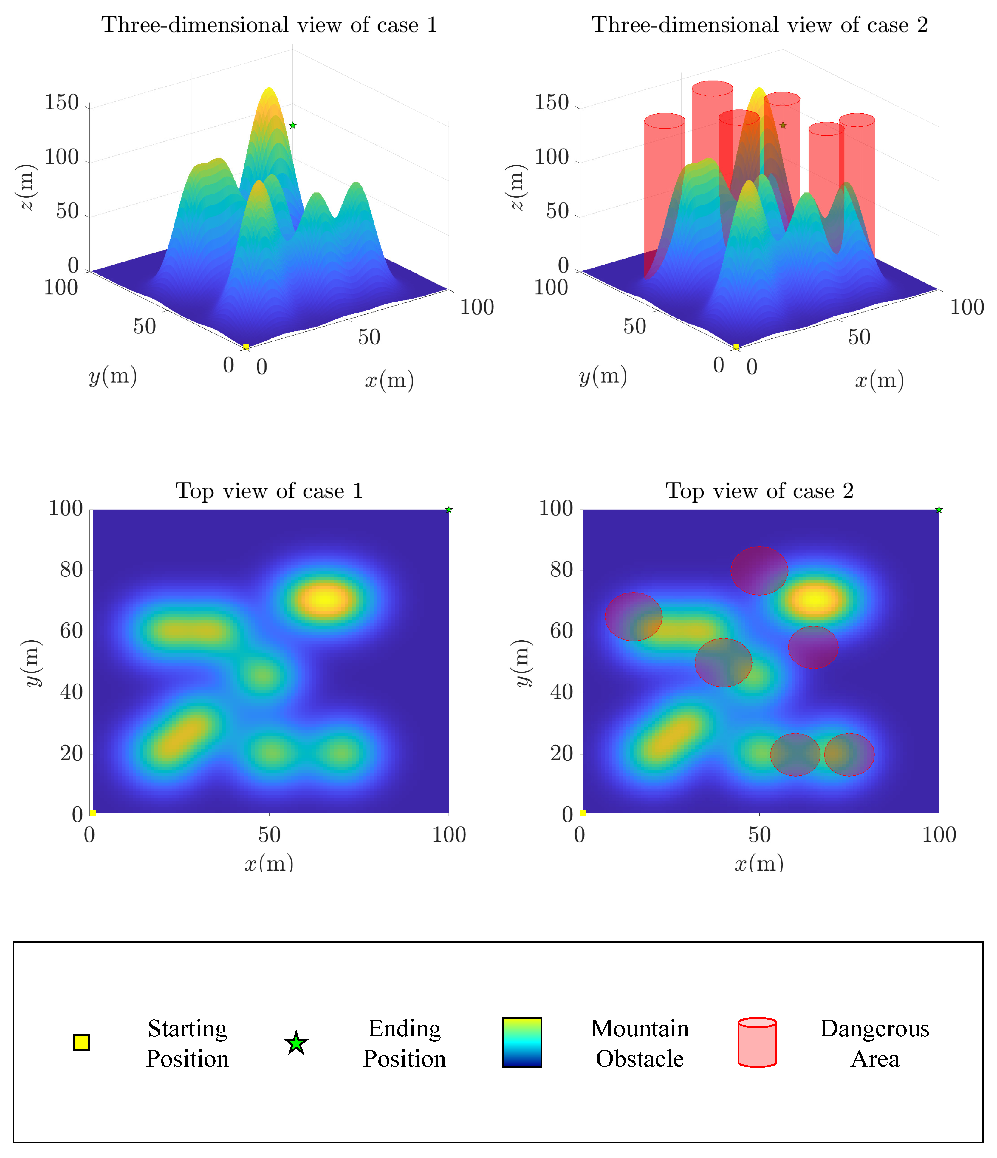
5.1. Problem Description

It is necessary to clarify the UAV mountain path-planning issue for achieving the mission goal in UAV mountain path planning. Missions like disaster rescue and military reconnaissance often involve the UAV mountain path-planning problem. The UAV mountain path-planning problem requires generating the minimum-distance path connecting the starting position and the ending position while avoiding the infeasible obstacle area and the threatening dangerous area. This ensures that the UAV can safely complete the assigned mission along the planned path with the lowest energy consumption.

To achieve the above goal and validate the practicality of DHSMEO in UAV mountain path-planning issue, the three-dimensional mountain map associated with this problem needs to be constructed at first. According to the stated goal, the three-dimensional mountain map needs to account for the infeasible mountain terrain and the threatening dangerous area. The model used to generate the mountain terrain in the three-dimensional mountain map is given via the following equation:

$$\begin{array}{c}\hfill z=\sum _{u=1}^U{h}_{u}exp[-{\left({\displaystyle \frac{x-x_u}{x_{\mathrm{p}\left(u\right)}}}\right)}^2-{\left({\displaystyle \frac{y-y_u}{y_{\mathrm{p}\left(u\right)}}}\right)}^2],\end{array}$$

(23)

where the following applies: z represents the height in a three-dimensional landscape; x and y represent the coordinates for horizontal points in a three-dimensional landscape; U is the number of peaks in the three-dimensional terrain; $x_u$ and $y_u$ are the coordinates of the u-th mountain peak; $h_u$ denotes the mountain contour of the u-th mountain peak; and $x_{\mathrm{p}\left(u\right)}$ and $y_{\mathrm{p}\left(u\right)}$ are the mountain contour parameters of the u-th mountain peak.

The threatening, dangerous area in the three-dimensional mountain map is modeled as a cylindrical region, which is used to represent the dangerous area commonly encountered in UAV mountain path-planning missions, such as the high-temperature fire zone in disaster rescue and the radar detection zone in military reconnaissance. The model used to generate the threatening, dangerous area is shown in the following equation:

$$\begin{array}{c}\hfill Threa{t}_v=(x_v,y_v,z_v,R_v),\end{array}$$

(24)

where $Threa{t}_v$ represents the v-th dangerous cylindrical region; $x_v$ and $y_v$ denote the horizontal and vertical coordinates for the center within the v-th dangerous cylindrical area, respectively; $z_v$ represents the height of the v-th dangerous cylindrical area; and $R_v$ represents the radius of the v-th dangerous cylindrical area. Compared to the infeasible mountain terrain, the interior of the dangerous cylindrical area is designated as infeasible, while its neighborhood area remains feasible but threatening.

Based on the aforementioned description of the UAV mountain path-planning problem, it is expressed with the below minimization problem to meet the mission requirements:

$$\begin{array}{cc}\hfill min\hfill & \hfill J_{\mathrm{UM}}=\parallel \mathit{Q}\parallel +{\eta }_{\mathrm{T}}{J}_{\mathrm{T}},\hfill \\ \hfill \mathrm{s}.\mathrm{t}.\hfill & \hfill \mathit{Q}\notin O_{\mathrm{b}},\hfill \end{array}$$

(25)

$$\begin{array}{c}\hfill J_{\mathrm{T}}=\sum _{k=1}^{K-1}\sum _{v=1}^V{J}_{\mathrm{T}(\mathrm{v},\mathrm{k})},\end{array}$$

(26)

$$\begin{array}{c}\hfill J_{\mathrm{T}(\mathrm{v},\mathrm{k})}=\left\{\begin{array}{cc}0,\hfill & d_{(v,k)}>D_v+R_v,\hfill \\ D_v+R_v-d_{(v,k)},\hfill & R_v<d_{(v,k)}\le D_v+R_v,\hfill \\ \infty ,\hfill & d_{(v,k)}\le R_v.\hfill \end{array}\right.\end{array}$$

(27)

where the following applies: $\mathit{Q}$ represents the three-dimensional path of a UAV connecting the initial position and the destination position; $J_{\mathrm{T}}$ represents the threat cost induced via the dangerous area; ${\eta }_{\mathrm{T}}$ denotes the weight associated with the threat cost; K represents the number of waypoints on a three-dimensional path; V denotes the number of cylindrical dangerous areas; $d_{(v,k)}$ represents the distance between the center of the v-th dangerous cylindrical area and the k-th segment of the three-dimensional path of UAV; $D_v$ represents the range of the threatening neighborhood area corresponding to the v-th dangerous cylindrical area; and $O_{\mathrm{b}}$ represents the infeasible areas formed by mountain obstacles.

5.2. DHSMEO-Based UAV Mountain Path-Planning Method

To handle the UAV mountain path-planning issue described by Section 5.1, as well as, ulteriorly, evaluating the practicality for DHSMEO, this subsection proposes a UAV mountain path-planning method that integrates a quasi-uniform cubic B-spline curve with DHSMEO.

A smooth path facilitates stable UAV flight. To meet this requirement, the B-spline curve method is adopted in constructing the smooth path of UAV [38]. The coordinates $(\mathit{Q}x\left(t\right),\mathit{Q}y\left(t\right),{\mathit{Q}}_z\left(t\right))$ of a UAV path in three-dimensional space generated via the B-spline curve method are calculated as follows:

$$\left\{\begin{array}{cc}\hfill {\mathit{Q}}_x\left(t\right)& \hfill =\sum _{h=0}^H{\mathit{x}}_h{B}_{h,M}\left(t\right),\hfill \\ \hfill {\mathit{Q}}_y\left(t\right)& \hfill =\sum _{h=0}^H{\mathit{y}}_h{B}_{h,M}\left(t\right),\hfill \\ \hfill {\mathit{Q}}_z\left(t\right)& \hfill =\sum _{h=0}^H{\mathit{z}}_h{B}_{h,M}\left(t\right),\hfill \end{array}\right.$$

(28)

where the following applies: $({\mathit{x}}_h,{\mathit{y}}_h,{\mathit{z}}_h)$ represents the coordinates of the $(h+1)$th control point of the B-spline curve; M is the order of the B-spline curve; and $B_{h,M}\left(t\right)$ is the B-spline basis function, which is defined by the following recursive formulas:

$$\begin{array}{c}\hfill \left\{\begin{array}{c}{B}_{h,M}\left(t\right)=\left\{\begin{array}{c}\hfill 1,t_h\le t<t_{h+1},\hfill \\ \hfill 0,\mathrm{otherwise},\hfill \end{array}\right. M=1,\hfill \\ B_{h,M}\left(t\right)={\displaystyle \frac{t-t_h}{t_{h+M-1}-t_h}}{B}_{h,M-1}\left(t\right)+{\displaystyle \frac{t_{h+M}-t}{t_{h+M}-t_{h+1}}}{B}_{h+1,M-1}\left(t\right),M\ge 2,\hfill \\ \mathrm{definition}{\displaystyle \frac{0}{0}}=0,\hfill \end{array}\right.\end{array}$$

(29)

where $t_h$ varies within the range $[t_0,t_1,\cdots ,t_{H+M}]$, whose values needs to satisfy $t_0\le t_1\le \cdots \le t_{H+M}$. Among different configurations of B-spline curves, the quasi-uniform cubic B-spline curve efficiently forms the smooth path by determining a small number of control points. It ensures that the obtained path crosses the starting and ending control points, and it allows for local modifications by adjusting the control points.

In sum, the specific steps involved in handling the UAV mountain path-planning issue using DHSMEO combined with the quasi-uniform cubic B-spline method are shown below:

Step 1. Initialize the three-dimensional mountain map $Map$ according to Equation (23).

Step 2. Initialize the path order, M, the number of control points, $H+1$, the starting position $({\mathit{x}}_0,{\mathit{y}}_0,{\mathit{z}}_0)$, and the ending position $({\mathit{x}}_H,{\mathit{y}}_H,{\mathit{z}}_H)$, along with other elements related to the UAV mountain path-planning problem.

Step 3. Initialize the current iteration number, l, the maximum iteration number, $l_{\max }$, the particle size, N, the particle dimension, $H+1$ (determined by the number of control points), and other related parameters required for DHSMEO.

Step 4. Construct the fitness function for DHSMEO in accordance with Equation (25).

Step 5. Determine control points of three-dimensional quasi-uniform cubic B-spline curve except the starting position and ending position using the concentration initialization strategy in DHSMEO, and form initial path via fitting the control points of three-dimensional quasi-uniform cubic B-spline curve.

Step 6. Optimize the control points from three-dimensional quasi-uniform cubic B-spline curve except the starting position and ending position in the generated path using DHSMEO to search the minimum-distance path connecting the starting position and ending position in a three-dimensional mountain map $Map$.

Step 7. Repeat Step 6 until the preset termination condition of DHSMEO is satisfied.

Step 8. Return the best path connecting the starting position and ending position.

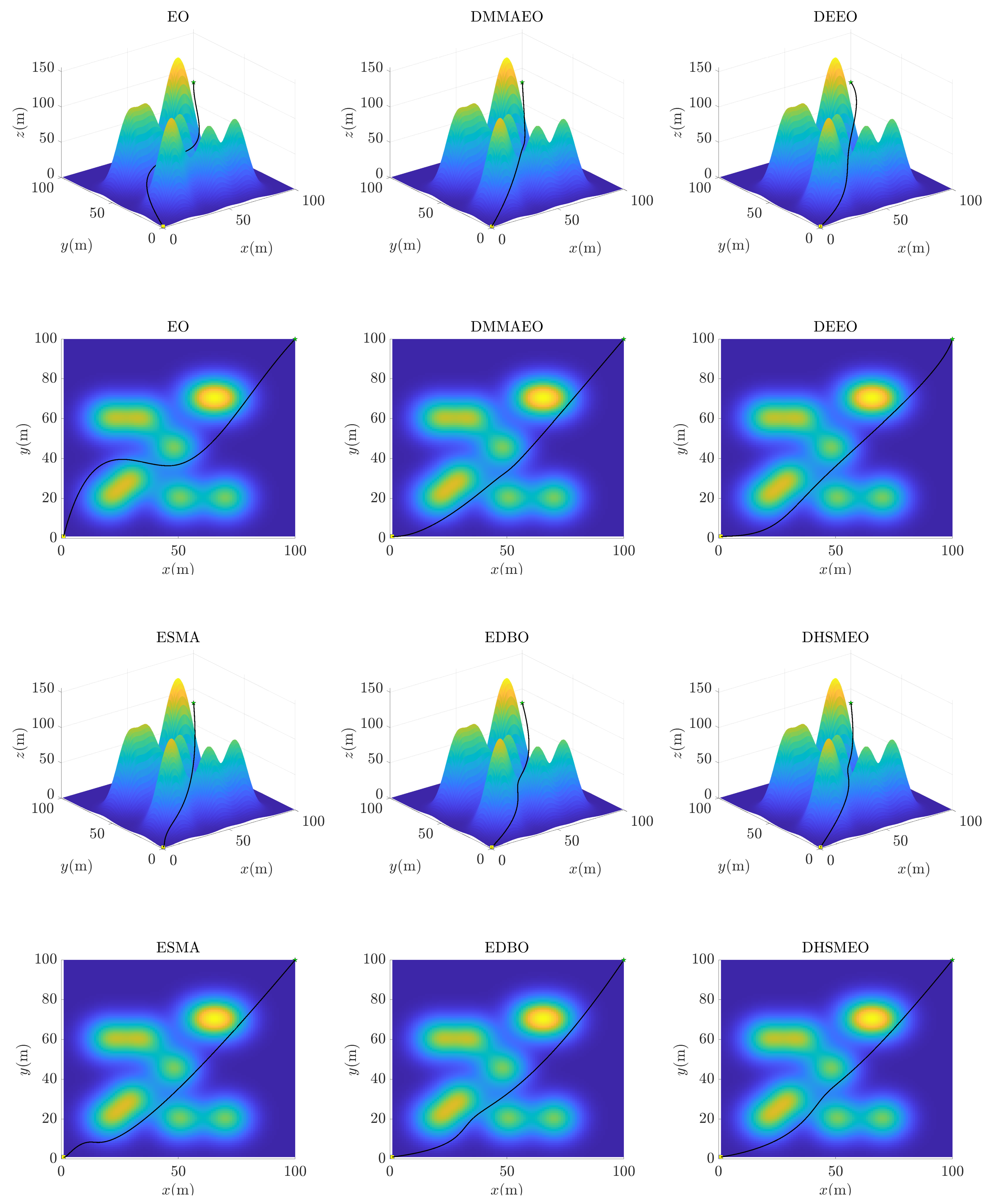
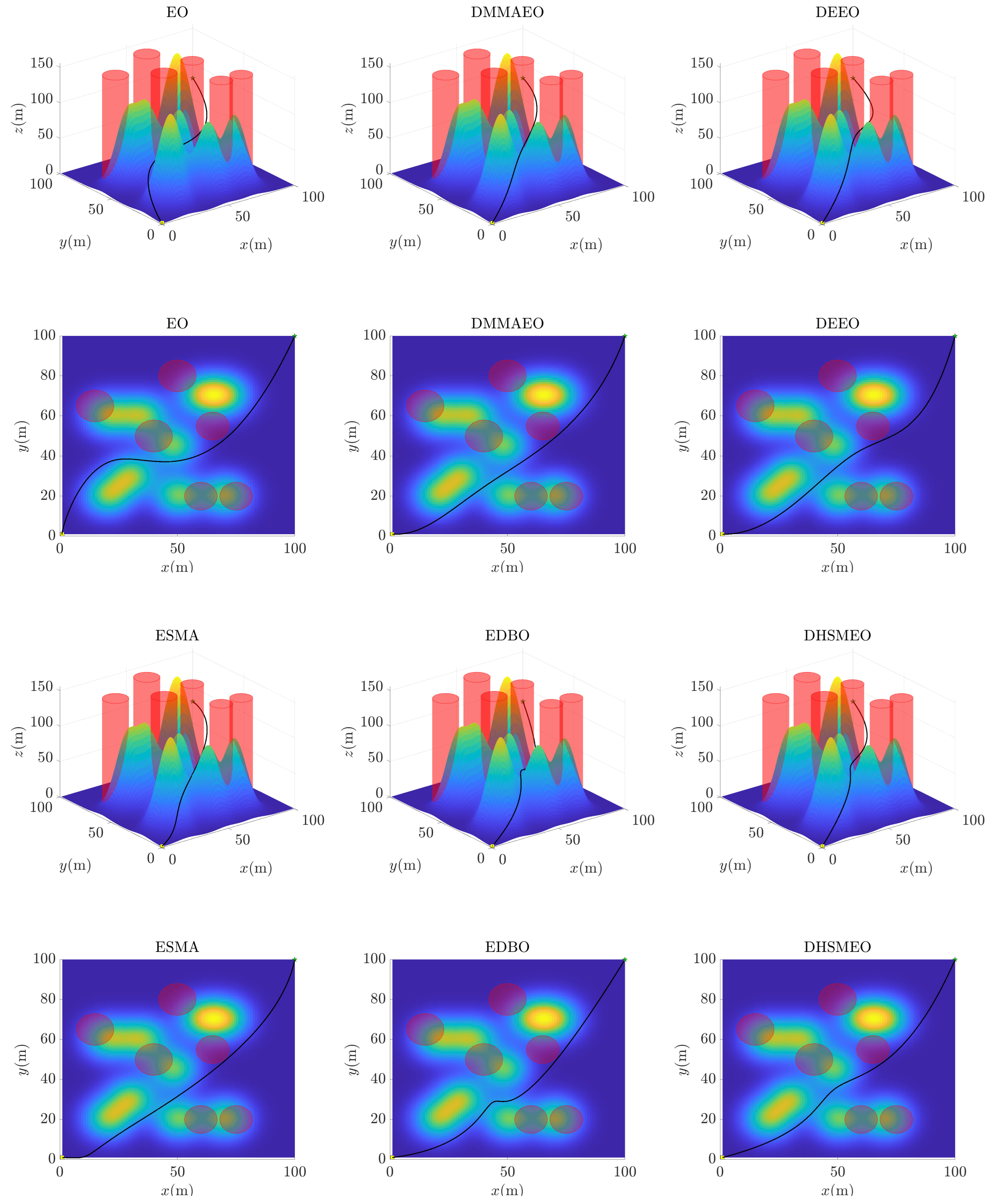
5.3. Results and Analysis of UAV Mountain Path Planning

To evaluate the practicality of DHSMEO, this section applies DHSMEO in addressing the UAV mountain path-planning problem. Additionally, the UAV mountain path-planning problem is also addressed by integrating other algorithms (EO [13], DMMAEO [21], DEEO [32], ESMA [34], and EDBO [39]) with the quasi-uniform cubic B-spline method in comparative performance analysis. The optimization performance of these algorithms is assessed through the best value (Best), average value (Avg), worst value (Worst), and standard deviation (Std). Among the comparative algorithms, EO serves as the original algorithm. DMMAEO, DEEO, and ESMA are the top three algorithms derived from the comparative experimental results of the previous section. And EDBO is a recently proposed algorithm for solving the UAV path-planning problem. The parameter configurations in the algorithms for the comparative analysis are derived from their original works.

According to different influencing factors in the UAV mountain path-planning environment, this subsection constructs two cases of three-dimensional mountain maps, which are shown in Figure 4. In the first case, a simple obstacle environment formed solely by the mountain terrain obstacle is considered. In the second case, a complex obstacle environment formed by a combination of the mountain terrain obstacle and the dangerous area is further considered. In these two cases of maps, the blue gradient area represents the infeasible mountain obstacle, the red cylindrical area indicates the threatening dangerous area, and the yellow square and green pentagram denote the starting position and the ending position of the UAV path-planning mission.

To ensure a fair evaluation of the performance of comparative algorithms in UAV mountain path planning, the comparative algorithms involved in this UAV mountain path-planning experiment adopt the same experimental configuration. Each algorithm is independently tested 30 times on the UAV mountain path-planning problem, and the results of the comparative algorithms are presented in

Table 15. Comparison results of UAV mountain path planning in case 1.

Algorithm	Best	Avg	Worst	Std
EO	179.1639	181.5920	188.3981	2.504409
DMMAEO	176.0768	179.1847	183.0997	1.957168
DEEO	176.2221	180.8633	185.6625	2.120665
ESMA	176.6373	180.6428	185.6273	2.013366
EDBO	175.7928	180.0901	185.5089	1.897720
DHSMEO	174.7972	177.2150	179.5667	1.750398

and

Table 16. Comparison results of UAV mountain path planning in case 2.

Algorithm	Best	Avg	Worst	Std
EO	180.4039	187.0131	188.6926	1.807976
DMMAEO	178.7315	186.2725	187.9656	1.721200
DEEO	180.3755	186.6118	187.6417	2.118246
ESMA	180.3311	186.3473	188.0306	1.834329
EDBO	178.5452	184.9253	186.3825	2.306150
DHSMEO	176.4555	178.8353	182.1692	1.692046

. In the comparative experimental results shown in Table 15 and Table 16, the top-performing results of the compared algorithms within the UAV mountain path-planning experiments are marked in bold. Figure 5 and Figure 6 further visualize the path-planning results of the comparative algorithms in the three-dimensional mountain map through black curves, which more intuitively reflect the capability of comparative algorithms to handle the UAV mountain path-planning issue.

In the first case with a simple obstacle environment, the UAV mountain path-planning issue needs to generate the shortest path connecting the starting position and the ending position in the fluctuating infeasible mountain terrain. Table 15 and Figure 5 illustrate the UAV mountain path-planning results of DHSMEO and other comparative algorithms under this case. The performance statistics of the comparative algorithms in handling the UAV mountain path-planning issue under the first case are summarized in Table 15. In accordance with the results from Table 15, the best value, average value, worst value, and standard deviation of DHSMEO are 175.3896, 178.1529, 179.9603, and 1.883847, respectively. These results of DHSMEO exhibit superior performance across all four evaluation indicators compared to other algorithms, and its optimization performance ranks first. The above analysis reveals that DHSMEO provides the most efficient optimization capability among the compared algorithms in the first UAV mountain path-planning case and shows the most competitive overall capability in terms of several indicators. Figure 5 further presents the three-dimensional view and the top view of the UAV mountain path-planning results obtained using the comparative algorithms in the first case. The comparison results in Figure 5 reveal that all the algorithms generate feasible paths in the fluctuating infeasible mountain terrain. However, the UAV path-planning results differ across the algorithms. Among the results obtained using the comparative algorithms, the standard EO is trapped in a local optimum, DHSMEO generates the shortest planning path, and other comparative algorithms generate different feasible paths within the same feasible corridor. The path-planning results shown in Figure 5 more intuitively highlight the performance differences among the comparative algorithms under the first UAV mountain path-planning case, and DHSMEO exhibits a better ability to address the UAV mountain path-planning problem than other comparison algorithms.

Unlike the first case with a simple obstacle environment, the second case with a complex obstacle environment requires considering the influence of the mountain terrain obstacle and the dangerous area on the generated path at the same time, which further enhances the difficulty of handling the UAV mountain path-planning issue. Table 16 and Figure 6 showcase the performance comparison of DHSMEO and other algorithms to handle the UAV mountain path-planning issue under this case. The statistical analysis for the comparative algorithms to handle the UAV mountain path-planning issue under this second case is provided in Table 16. Table 16 presents the performance of DHSMEO, with a best value of 176.4555, an average value of 178.8353, a worst value of 182.1692, and a standard deviation of 1.692046. These results remain better than those of the other comparative algorithms across all four performance indicators, and they make DHSMEO still rank first in optimization performance. Additionally, compared with the path-planning results for the compared algorithms in the first case from Table 15, the path-planning results from DHSMEO exhibit the least variation among the path-planning results for comparative algorithms in the second case from Table 16. The above results indicate that DHSMEO maintains its leading optimization performance among the compared algorithms to handle the UAV mountain path-planning issue under the second case with a complex obstacle environment, and it also shows the most stable and competitive overall performance among the comparison algorithms in terms of multiple indicators. Figure 6 further presents the three-dimensional view and the top view for the UAV mountain path-planning results derived from the comparative algorithms under the second scenario. As shown in Figure 6, compared to the paths generated in the first case, all comparative algorithms further adjust the path-planning results for the dangerous area and generate feasible paths to meet the needs of UAV mountain path planning in this case. Although the comparative algorithms adjust their path-planning results for the dangerous area, the standard EO still falls into a local optimum, and DHSMEO still generates the shortest planning path. The path-planning results shown in Figure 5 more intuitively show that DHSMEO still exhibits a better UAV mountain path-planning problem-solving capability among the comparative algorithms under the second case with a complex obstacle environment.

In sum, according to the experimental results of UAV mountain path planning presented in Table 15 and Table 16 and Figure 5 and Figure 6, the proposed DHSMEO provides practical and competitive optimization results for the UAV mountain path-planning problem across obstacle environments with different levels of complexity.

6. Conclusions

By analyzing the deficiencies of optimization strategy in the standard equilibrium optimizer (EO), a dynamic heterogeneous search-mutation structure-based equilibrium optimizer (DHSMEO) has been developed to address the issues of population diversity attenuation, insufficient search efficiency, and susceptibility to a local optimum in the EO. Firstly, a dynamic dual-subpopulation adaptive grouping strategy was constructed to form the construction mode of a dual-subpopulation structure, which can improve population diversity and provide an effective information-exchange structure for the heterogeneous hybrid search strategy. Then, a heterogeneous hybrid search-based concentration-updating strategy was introduced into the formed dual-subpopulation structure to form a differentiated population search strategy, which can enhance search efficiency. Finally, a dynamic Levy mutation was applied in the optimal equilibrium candidate, serving as the central hub of the algorithm guidance strategy to leverage the unique randomness of dynamic Levy mutation in refining the optimal equilibrium candidate, which can strengthen the ability of escaping local optima.

Three sets of comparative experiments were conducted on 39 typical benchmark functions and a UAV mountain path-planning problem to evaluate the overall optimization capability of DHSMEO. The effectiveness analysis results for improvement strategies suggest that the dynamic dual-subpopulation adaptive grouping strategy, the heterogeneous hybrid search-based concentration-updating strategy, and the dynamic Levy mutation-based optimal equilibrium candidate-refining strategy constructed in DHSMEO all contribute to enhancing the optimization capability. And DHSMEO obtained by combining these three improvement strategies simultaneously to form the dynamic heterogeneous search-mutation structure achieves the best optimization performance. In further comparative experiments with other algorithms, DHSMEO achieved a better optimization capability across most benchmark functions than other algorithms, and it showed superiority in overall optimization performance. Additionally, in the comparison experiments for the UAV mountain path-planning problem, DHSMEO effectively solved the UAV mountain path-planning problem, and it exhibited superiority compared to other algorithms, which shows both practicality and competitiveness in addressing the UAV mountain path-planning problem.

With the achievements of DHSMEO, future research on DHSMEO will focus on further enhancing its optimization performance and expanding its applicability. Firstly, improving its adaptability to large-scale optimization problems will be a key direction, which will ensure its efficiency in searching high-dimensional complex optimization space. Moreover, extending DHSMEO to address discrete and multi-objective optimization problems will be studied, which will make it applicable to broader application challenges. Additionally, the application of DHSMEO in more kinds of practical optimization problems will be further investigated, including smart grid scheduling, building structure optimization, and medical image processing, etc. DHSMEO is expected to provide more efficient and reliable solutions in various engineering and scientific domains.

References

1. Huang, W.; Liu, H.; Zhang, Y.; Mi, R.; Tong, C.; Xiao, W.; Shuai, B. Railway dangerous goods transportation system risk identification: Comparisons among SVM, PSO-SVM, GA-SVM and GS-SVM. Appl. Soft Comput. 2021, 109, 107541. [Google Scholar] [CrossRef]
2. Avalos, O.; Haro, E.H.; Camarena, O.; Díaz, P. Improved crow search algorithm for optimal flexible manufacturing process planning. Expert Syst. Appl. 2024, 235, 121243. [Google Scholar] [CrossRef]
3. Alweshah, M.; Alkhalaileh, S.; Al-Betar, M.A.; Bakar, A.A. Coronavirus herd immunity optimizer with greedy crossover for feature selection in medical diagnosis. Knowl.-Based Syst. 2022, 235, 107629. [Google Scholar] [CrossRef] [PubMed]
4. Zhao, X.D.; Fang, Y.M.; Liu, L.; Xu, M.; Zhang, P. Ameliorated moth-flame algorithm and its application for modeling of silicon content in liquid iron of blast furnace based fast learning network. Appl. Soft Comput. 2020, 94, 106418. [Google Scholar] [CrossRef]
5. Xie, X.; Yang, Y.L.; Zhou, H. Multi-Strategy Hybrid Whale Optimization Algorithm Improvement. Appl. Sci. 2025, 15, 2224. [Google Scholar] [CrossRef]
6. Chen, Q.; Qu, H.; Liu, C.; Xu, X.; Wang, Y.; Liu, J. Spontaneous coal combustion temperature prediction based on an improved grey wolf optimizer-gated recurrent unit model. Energy 2025, 314, 133980. [Google Scholar] [CrossRef]
7. Gharehchopogh, F.S.; Ucan, A.; Ibrikci, T.; Arasteh, B.; Isik, G. Slime mould algorithm: A comprehensive survey of its variants and applications. Arch. Comput. Methods Eng. 2023, 30, 2683–2723. [Google Scholar] [CrossRef]
8. Faris, H.; Aljarah, I.; Al-Betar, M.A.; Mirjalili, S. Grey wolf optimizer: A review of recent variants and applications. Neural Comput. Appl. 2018, 30, 413–435. [Google Scholar] [CrossRef]
9. Yang, Y.T.; Chen, H.L.; Heidari, A.A.; Gandomi, A.H. Hunger games search: Visions, conception, implementation, deep analysis, perspectives, and towards performance shifts. Expert Syst. Appl. 2021, 177, 114864. [Google Scholar] [CrossRef]
10. Houssein, E.H.; Gad, A.G.; Hussain, K.; Suganthan, P.N. Major advances in particle swarm optimization: Theory, analysis, and application. Swarm Evol. Comput. 2021, 63, 100868. [Google Scholar] [CrossRef]
11. Abualigah, L.; Abd Elaziz, M.; Sumari, P.; Geem, Z.W.; Gandomi, A.H. Reptile Search Algorithm (RSA): A nature-inspired meta-heuristic optimizer. Expert Syst. Appl. 2022, 191, 116158. [Google Scholar] [CrossRef]
12. Ahmad, M.F.; Isa, N.A.M.; Lim, W.H.; Ang, K.M. Differential evolution: A recent review based on state-of-the-art works. Alex. Eng. J. 2022, 61, 3831–3872. [Google Scholar] [CrossRef]
13. Faramarzi, A.; Heidarinejad, M.; Stephens, B.; Mirjalili, S. Equilibrium optimizer: A novel optimization algorithm. Knowl.-Based Syst. 2020, 191, 105190. [Google Scholar] [CrossRef]
14. Shaik, M.A.; Mareddy, P.L. Enhancement of Voltage Profile in the Distribution system by Reconfiguring with DG placement using Equilibrium Optimizer. Alex. Eng. J. 2022, 61, 4081–4093. [Google Scholar] [CrossRef]
15. Wu, X.D.; Hirota, K.; Jia, Z.Y.; Ji, Y.; Zhao, K.X.; Dai, Y.P. Ameliorated equilibrium optimizer with application in smooth path planning oriented unmanned ground vehicle. Knowl.-Based Syst. 2023, 260, 110148. [Google Scholar] [CrossRef]
16. Rabehi, A.; Nail, B.; Helal, H.; Douara, A.; Ziane, A.; Amrani, M.; Akkal, B.; Benamara, Z. Optimal estimation of Schottky diode parameters using advanced swarm intelligence algorithms. Semiconductors 2020, 54, 1398–1405. [Google Scholar] [CrossRef]
17. Fan, Q.S.; Huang, H.S.; Yang, K.; Zhang, S.S.; Yao, L.G.; Xiong, Q.Q. A modified equilibrium optimizer using opposition-based learning and novel update rules. Expert Syst. Appl. 2021, 170, 114575. [Google Scholar] [CrossRef]
18. Tang, A.D.; Han, T.; Zhou, H.; Xie, L. An improved equilibrium optimizer with application in unmanned aerial vehicle path planning. Sensors 2021, 21, 1814. [Google Scholar] [CrossRef]
19. Dinkar, S.K.; Deep, K.; Mirjalili, S.; Thapliyal, S. Opposition-based Laplacian equilibrium optimizer with application in image segmentation using multilevel thresholding. Expert Syst. Appl. 2021, 174, 114766. [Google Scholar] [CrossRef]
20. Wunnava, A.; Naik, M.K.; Panda, R.; Jena, B.; Abraham, A. A novel interdependence based multilevel thresholding technique using adaptive equilibrium optimizer. Eng. Appl. Artif. Intel. 2020, 94, 103836. [Google Scholar] [CrossRef]
21. Wu, X.D.; Hirota, K.; Dai, Y.P.; Shao, S. Dynamic Multi-Population Mutation Architecture-Based Equilibrium Optimizer and Its Engineering Application. Appl. Sci. 2025, 15, 1795. [Google Scholar] [CrossRef]
22. Abdel-Basset, M.; Mohamed, R.; Mirjalili, S.; Chakrabortty, R.K.; Ryan, M.J. Solar photovoltaic parameter estimation using an improved equilibrium optimizer. Sol. Energy 2020, 209, 694–708. [Google Scholar] [CrossRef]
23. Hemavathi, S.; Latha, B. HFLFO: Hybrid fuzzy levy flight optimization for improving QoS in wireless sensor network. Ad Hoc Networks 2023, 142, 103110. [Google Scholar] [CrossRef]
24. Xu, Y.; Chen, H.; Heidari, A.A.; Luo, J.; Zhang, Q.; Zhao, X.; Li, C. An efficient chaotic mutative moth-flame-inspired optimizer for global optimization tasks. Expert Syst. Appl. 2019, 129, 135–155. [Google Scholar] [CrossRef]
25. Muthusamy, H.; Ravindran, S.; Yaacob, S.; Polat, K. An improved elephant herding optimization using sine–cosine mechanism and opposition based learning for global optimization problems. Expert Syst. Appl. 2021, 172, 114607. [Google Scholar] [CrossRef]
26. Feng, Z.; Duan, J.; Niu, W.; Jiang, Z.; Liu, Y. Enhanced sine cosine algorithm using opposition learning, adaptive evolution and neighborhood search strategies for multivariable parameter optimization problems. Appl. Soft Comput. 2022, 119, 108562. [Google Scholar] [CrossRef]
27. Zhong, C.T.; Li, G.; Meng, Z. Beluga whale optimization: A novel nature-inspired metaheuristic algorithm. Knowl.-Based Syst. 2022, 251, 109215. [Google Scholar] [CrossRef]
28. Shami, T.M.; Mirjalili, S.; Al-Eryani, Y.; Daoudi, K.; Izadi, S.; Abualigah, L. Velocity pausing particle swarm optimization: A novel variant for global optimization. Neural Comput. Appl. 2023, 35, 9193–9223. [Google Scholar] [CrossRef]
29. Liang, J.J.; Suganthan, P.N.; Deb, K. Novel Composition Test Functions for Numerical Global Optimization. In Proceedings of the 2005 IEEE Swarm Intelligence Symposium, Pasadena, CA, USA, 8–10 June 2005; pp. 68–75. [Google Scholar]
30. Maharana, D.; Kommadath, R.; Kotecha, P. Dynamic Yin-Yang Pair Optimization and Its Performance on Single Objective Real Parameter Problems of CEC 2017. In Proceedings of the 2017 IEEE Congress on Evolutionary Computation (CEC 2017), San Sebastián, Spain, 5–8 June 2017; pp. 2390–2396. [Google Scholar]
31. Faramarzi, A.; Heidarinejad, M.; Mirjalili, S.; Gandomi, A.H. Marine Predators Algorithm: A nature-inspired metaheuristic. Expert Syst. Appl. 2020, 152, 113377. [Google Scholar] [CrossRef]
32. Moharam, A.; Haikal, A.Y.; Elhosseini, M. Economically optimized heat exchanger design: A synergistic approach using differential evolution and equilibrium optimizer within an evolutionary algorithm framework. Neural Comput. Appl. 2024, 36, 14999–15026. [Google Scholar] [CrossRef]
33. Almotairi, K.H.; Abualigah, L. Hybrid reptile search algorithm and remora optimization algorithm for optimization tasks and data clustering. Symmetry 2022, 14, 458. [Google Scholar] [CrossRef]
34. Naik, M.K.; Panda, R.; Abraham, A. An entropy minimization based multilevel colour thresholding technique for analysis of breast thermograms using equilibrium slime mould algorithm. Appl. Soft Comput. 2021, 113, 107955. [Google Scholar] [CrossRef]
35. Mahajan, S.; Abualigah, L.; Pandit, A.K. Hybrid arithmetic optimization algorithm with hunger games search for global optimization. Multimed. Tools Appl. 2022, 81, 28755–28778. [Google Scholar] [CrossRef]
36. Wang, H.; Wu, Z.J.; Rahnamayan, S.; Liu, Y.; Ventresca, M. Enhancing particle swarm optimization using generalized opposition-based learning. Inform. Sci. 2011, 181, 4699–4714. [Google Scholar] [CrossRef]
37. Xu, Y.; Chen, H.; Luo, J.; Zhang, Q.; Jiao, S.; Zhang, X. Enhanced Moth-flame optimizer with mutation strategy for global optimization. Inform. Sci. 2019, 492, 181–203. [Google Scholar] [CrossRef]
38. Wang, P.W.; Yang, J.S.; Zhang, Y.L.; Wang, Q.W.; Sun, B.B.; Guo, D. Obstacle-Avoidance Path-Planning Algorithm for Autonomous Vehicles Based on B-Spline Algorithm. World Electr. Veh. J. 2022, 13, 233. [Google Scholar] [CrossRef]
39. Yu, M.Y.; Du, J.; Xu, X.X.; Xu, J.; Jiang, F.; Fu, S.W.; Zhang, J.; Liang, A. A multi-strategy enhanced Dung Beetle Optimization for real-world engineering problems and UAV path planning. Alex. Eng. J. 2025, 118, 406–434. [Google Scholar] [CrossRef]
Figure 1. Flowchart of DHSMEO.
Applsci 15 05252 g001
Figure 2. Convergence curves of different improvement strategies in six benchmark functions.
Applsci 15 05252 g002
Figure 3. Convergence curves of DHSMEO and other algorithms in six benchmark functions.
Applsci 15 05252 g003
Figure 4. Three-dimensional mountain map.
Applsci 15 05252 g004
Figure 5. UAV mountain path-planning results of compared algorithms in case 1.
Applsci 15 05252 g005
Figure 6. UAV mountain path-planning results of compared algorithms in case 2.
Applsci 15 05252 g006