Machine Selection for Inventory Tracking with a Continuous Intuitionistic Fuzzy Approach

Abstract

Today, businesses are adopting digital transformation strategies to make their production processes more agile, efficient, and sustainable. At the same time, lean manufacturing principles aim to create value by reducing waste in production processes. In this context, it is important that the machine to be selected for inventory tracking can meet both the technological features suitable for digital transformation goals and the operational efficiency criteria required by lean manufacturing. In this study, multi-criteria decision-making methods were used to select the most suitable machine for inventory tracking based on digital transformation and lean manufacturing perspectives. This study applies a framework that integrates the Continuous Intuitionistic Fuzzy Analytic Hierarchy Process (CINFU AHP) and the Continuous Intuitionistic Fuzzy Combinative Distance-Based Assessment (CINFU CODAS) methods to select the most suitable machine for inventory tracking. The framework contributes to lean manufacturing by providing actionable insights and robust sensitivity analyses, ensuring decision-making reliability under fluctuating conditions. The CINFU AHP method determines the relative importance of each criterion by incorporating expert opinions. Six criteria, Speed (C1), Setup Time (C2), Ease to Operate and Move (C3), Ability to Handle Multiple Operations (C4), Maintenance and Energy Cost (C5), and Lifetime (C6), were considered in the study. The most important criteria were C1 and C4, with scores of 0.25 and 0.23, respectively. Following the criteria weighting, the CINFU CODAS method ranks the alternative machines based on their performance across the weighted criteria. Four alternative machines (High-Speed Automated Scanner (A1), Multi-Functional Robotic Arm (A2), Mobile Inventory Tracker (A3), and Cost-Efficient Fixed Inventory Counter (A4)) are evaluated based on the criteria selected. The results indicate that Alternative A1 ranked first because of its superior speed and operational efficiency, while Alternative A3 ranked last due to its high initial cost despite being cost-effective. Finally, a sensitivity analysis further examines the impact of varying criteria weights on the alternative rankings. Quantitative findings demonstrate how the applied CINFU AHP&CODAS methodology influenced the rankings of alternatives and their sensitivity to criteria weights. The results revealed that C1 and C4 were the most essential criteria, and Machine A2 outperformed others under varying weights. Sensitivity results indicate that the changes in criterion weights may affect the alternative ranking.

1. Introduction

Today, the e-integration of digital solutions is essential to maintain a competitive advantage. Even if digital solutions developed to manage systems that are parts of the whole fulfill their tasks individually, they can fully ensure organizational integrity when they work together [1]. Although digital systems play a central role in collecting and organizing production data and using them for processes such as planning and analysis, they often lack real-time tracking to count raw materials and semi-finished goods in stock [2]. Despite advances, accurate counting of raw materials and semi-finished products continues to pose challenges. Traditional manual counting methods are prone to errors and inefficiencies, necessitating a comprehensive and integrated approach to address the plate counting problem effectively. These limitations can lead to inaccuracies in inventory counts and cause wasted resources, delayed production, and inefficiencies that directly impact operational costs and productivity [3].

For this reason, companies have adopted lean manufacturing principles to reduce waste, increase efficiency, and build flexibility in their production processes. Lean manufacturing provides a structured procedure to pinpoint and minimize waste but requires a complementary system to integrate and operationalize these principles in real time [4]. Connecting digital solutions with lean techniques presents a promising way to achieve high accuracy and control in inventory and production management.

However, integrating digital solutions and initiatives of lean manufacturing techniques alone is insufficient to achieve optimal results [5]. A holistic approach that includes multifaceted decision-making and strategic planning is essential. A collaborative practice operating the Analytic Hierarchy Process (AHP) and Combinative Distance-Based Assessment (CODAS) methods presents considerable potential to tackle the complicated challenges of machine selection. AHP feeds a systematic framework for hierarchically analyzing and ranking machine alternatives, considering various factors [6]. In parallel, CODAS supports decision making by effectively ranking these alternatives, allowing for uncertainties and ambiguities that often arise in complex scenarios [7].

Combining AHP and CODAS yields a strong synergy, connecting AHP’s structured examination of decision criteria via hierarchical levels and pairwise comparisons with CODAS’s strength in addressing complicated, ambiguous and inconsistent information [8]. AHP enables the framework by representing the decision criteria and their relative importance. At the same time, CODAS enriches it by assessing and ranking alternatives on these criteria, accounting for inherent uncertainties and interdependencies. This collaborative approach allows decision-makers in manufacturing industry to guide the complexities of machine selection effectively, enabling well-informed consideration of alternatives [9].

The fuzzy extensions, in particular, improve the multi-criteria decision-making (MCDM) process, facilitating more effective navigation of the complexities in machine selection. The study utilized the Continuous Intuitionistic Fuzzy Analytic Hierarchy Process (CINFU AHP) for criteria weighting and Continuous Intuitionistic Fuzzy Combinative Distance-Based Assessment (CINFU CODAS) for alternative ranking. AHP was chosen for its effectiveness in accurately assigning weights to criteria through expert evaluations via pairwise comparisons. Although traditionally applied to multi-level hierarchies, AHP is also highly applicable for single-level criteria weighting, which aligns with the purpose of this research [10]. This study’s criteria represent a single-level structure, eliminating the need for sub-criteria. AHP was used solely to derive the weights of these criteria, which were then input into the CODAS method for alternative ranking. CODAS was selected for its capability to rank alternatives based on their performance across weighted criteria, utilizing both Euclidean and Taxicab distances for evaluation. This integration approach balances methodological simplicity with robust decision-making, ensuring the reliability of the results while avoiding unnecessary complexity. Its fuzzy extension enhances decision-making under uncertainty, complementing AHP by effectively managing alternative assessments. The integration of these methods provides a comprehensive framework for addressing the machine selection problem [11,12].

Since 1975, there have been many fuzzy set extensions introduced by researchers, such as Type-2 fuzzy sets [13], Pythagorean fuzzy sets [14,15], and Spherical fuzzy sets [16] to illustrate and protect uncertainty more reasonably. The Continuous Intuitionistic Fuzzy Set (CINFUS) is one of the recent extensions seeking to define continuous and uncertain information in real-world decision-making problems more accurately. It allows issues managed within a specific continuity scope to be more accurately modeled. CINFUSs, which have a more flexible structure than other fuzzy set extensions, permit more complicated systems to be modeled. Moreover, CINFUS, by classifying and considering decision-makers’ behavior against uncertainty as risk-averse, risk-neutral, or risk-taking, also enables examination of the data including the uncertainty introduced by decision-makers [17,18].

This research investigates how to combine lean manufacturing principles with digital transformation objectives in the machine selection process for managing inventory. Lean manufacturing prioritizes the removal of waste, enhancement of efficiency, and provision of value, whereas digital transformation facilitates real-time data integration, automation, and predictive analytics. The suggested decision-making framework integrates these principles through thoughtfully chosen evaluation criteria, ensuring alignment with goals related to operational efficiency and technological progress. This integration addresses the changing requirements of contemporary manufacturing settings, where agility, scalability, and cost-effectiveness are essential. Existing machine selection strategies frequently struggle with handling uncertainties and ambiguities inherent in decision-maker evaluations and criteria weighting. By integrating the Continuous Intuitionistic Fuzzy Analytic Hierarchy Process (CINFU AHP) and Continuous Intuitionistic Fuzzy Combinative Distance-Based Assessment (CINFU CODAS), this study bridges the gap, offering a structured, reliable, and sensitivity-tested framework for managing multi-criteria trade-offs, thereby reassuring the audience of its comprehensive approach.

The following key research questions (RQs) have been formulated to guide the study:

RQ 1: How can integrating CINFU AHP and CODAS methods enhance decision-making under conditions of uncertainty and ambiguity compared to traditional methods? This question explores the value added by combining fuzzy multi-criteria decision-making techniques, with a focus on their ability to accommodate vague or imprecise data in expert evaluations and to ensure consistency in ranking alternatives.

RQ 2: What are the most critical criteria influencing machine selection for inventory tracking within lean manufacturing systems? This question seeks to identify and prioritize the operational and technological factors, such as speed, setup time, ease of operation, energy cost, and maintenance, essential for selecting machines that align with efficiency and sustainability objectives.

RQ 3: How does modifying the significance of criteria through sensitivity analysis affect the ranking of machine alternatives? This question investigates the framework’s robustness under varying weighting scenarios, demonstrating its applicability in dynamic decision-making environments where priorities may shift.

The rest of the paper is organized as follows: Section 2 reviews related work to reveal the gap in the literature. Section 3 introduces the preliminaries and basics of the CINFUS approach, starting from intuitionistic fuzzy sets. Section 4 presents the applied methodology, CINFU AHP and CODAS. Section 5 describes the case study to show the applied results of the methodology. Section 6 presents the sensitivity analysis results to show how the ranking results are sensitive to the criteria weights. Section 7 compares the results with a non-fuzzy AHP and CODAS method. Finally, Section 8 concludes the study by discussing limitations and future work.

2. Literature Review

Inventory management is an essential aspect of manufacturing systems, playing a crucial role in enhancing operational efficiency and satisfying customer demand. Traditional inventory management methods often depend on periodic assessments and manual tracking, which can lead to inefficiencies and delays. In contrast, digital systems harness technological advancements to provide real-time visibility and automation in inventory management processes [19]. Research has shown the substantial impact of IoT (Internet of Things) applications on inventory management within lean manufacturing systems [20,21,22]. By integrating IoT technologies with lean principles, manufacturers can reduce waste, optimize resource utilization, and improve efficiency. For instance, IoT devices can track material movement within a facility, eliminating unnecessary transportation and storage waste—critical concerns in lean manufacturing [23]. Furthermore, IoT systems enable predictive maintenance of inventory management equipment, resulting in reduced downtime and enhanced equipment reliability, aligning with lean and digital transformation goals [24]. For example, Fatima [25] considered the applications of IoT across different industrial sectors, outlining the key technologies, benefits, and challenges associated with its implementation. Fang et al. [26] showed that sensor-based monitoring systems improve inventory accuracy. However, these studies were generally limited to a specific product type and did not propose an integrated system. Powell [27] examined the potential of integrating Enterprise Resource Planning (ERP) systems as a digital solution with lean manufacturing principles to achieve a competitive advantage for manufacturers. The authors argued that modern systems could support lean principles despite traditional viewpoints that see ERP as a hindrance to these. Abobakr et al. [5] investigated the impact of integrating digital systems and lean manufacturing practices on a company’s sustainability performance. The main finding was that integrating both practices significantly improves overall sustainability performance.

The fusion of digital transformation technologies and lean manufacturing principles generates a powerful synergy that significantly improves efficiency, flexibility, and sustainability in modern production systems [28]. Lean manufacturing minimizes waste and maximizes value by optimizing operations and enhancing resource utilization. Digital technologies, such as the Internet of Things (IoT), complement these objectives by addressing traditional challenges and facilitating more intelligent decision-making processes [29].

IoT devices play a vital role in waste reduction by providing real-time insights into inventory levels, material movement, and production status. This immediate visibility helps to minimize overproduction, waiting times, and unnecessary transportation, perfectly aligning with lean principles [30,31]. Flexibility and adaptability, cornerstones of lean manufacturing, are further augmented by digital platforms and tools. This integration enhances responsiveness and enables the seamless coordination of resources, thereby improving overall system efficiency [32].

While digitalization has improved inventory management and lean manufacturing, there are still significant challenges in accurate counting because of the variety in technology [33,34]. These advancements emphasize the need for decision-making frameworks incorporating digital capabilities in evaluating and selecting inventory management systems. Some studies focused on various decision-making models for lean manufacturing or inventory management systems as a part of lean principles. Anand and Kodali [35] aimed to explain how companies make the strategic decision to choose lean manufacturing systems as part of their manufacturing strategy and on what basis managers make such strategic decisions. A comprehensive analysis of the PROMETHEE (Preference Ranking for Organization Method for Enrichment Evaluations) model reveals that lean systems were the best model for the given case conditions. Since a single case study approach was used, the findings cannot be generalized to any other industry without sensitivity analysis. Zhu et al. [36] applied fuzzy AHP-DEMATEL (Decision Making Trial and Evaluation Laboratory) to analyze the relationship between indicators and the structure of the indicator system. The complex network formed by the indicator system is divided into different levels. Some studies applied fuzzy decision-making methods to improve results. For example, Buonamico et al. [37] showed that using a tool based on fuzzy logic-based metrics supported achieving lean warehousing management goals, such as waste elimination and cross-functional teams and empowerment. Es et al. [4] explored how to select the best material-handling equipment for a lean manufacturing system. The authors proposed using the Hesitant Fuzzy Analytic Hierarchy Process in a case study where the goal was to choose between different material-handling equipment.

2.1. Contribution of the Study

This study’s contribution can be considered from three perspectives with regard to the literature: application area, decision-making technique, and approach.

2.1.1. Application Area

The studies in the literature present valuable insights into the principles and practices of lean manufacturing, mainly focusing on the significance of waste reduction and process optimization [38,39]. While the studies mostly concentrate on material handling within a lean system, the principles discussed can be extrapolated to selecting all types of machinery utilized in lean manufacturing environments.

Deciding on the right machinery is critical in launching a successful lean manufacturing approach [35]. This decision should be taken seriously and needs a thorough evaluation procedure considering multiple criteria. Some factors, such as machine capabilities, integration with other systems, cost-effectiveness, and sustainability, must be carefully considered. For example, a machine’s ability to meet required production volumes and quality standards is paramount. Additionally, seamless integration with existing production systems and data infrastructure is crucial for achieving the data-driven decision-making that characterizes modern lean systems.

2.1.2. Decision-Making Technique

This research contributes to the literature by integrating a hybrid fuzzy MDCM technique (CINFU AHP and CINFU CODAS) under lean principles specifically for machine selection in inventory tracking to answer predefined research questions. It presents the optimized decision-making process under uncertainty by conducting a case study demonstrating the practical implementation and benefits of the proposed framework in real-world scenarios. Moreover, it applies sensitivity analysis to decrease subjectivity and test the what-if conditions.

While the individual methods utilized in this study, CINFU AHP and CINFU CODAS, are not entirely novel, their customized integration into a specific industrial challenge, machine selection for inventory tracking, contributes to MCDM. In contrast to prior applications, the criteria and decision model developed in this research reflect the priorities of lean manufacturing and digital transformation. Including comprehensive sensitivity analysis further differentiates this work, providing a valuable tool for decision-makers. By validating the framework through a real-world case study, this research effectively bridges the gap between theoretical models and industrial practice, offering a replicable approach for tackling similar challenges in other manufacturing contexts.

2.1.3. Approach

The study approaches the research based on several critical research questions to deepen the reader’s understanding. RQ 1 explores how integrating CINFU AHP and CODAS methods can enhance decision-making under conditions of uncertainty and ambiguity compared to traditional methods. This question focuses on the value added by combining fuzzy multi-criteria decision-making techniques, specifically their ability to accommodate vague or imprecise data in expert evaluations and to ensure consistency in ranking alternatives. RQ 2 investigates the most critical criteria influencing machine selection for inventory tracking within lean manufacturing systems. This question identifies and prioritizes operational and technological factors, such as speed, setup time, ease of operation, energy cost, and maintenance, which are essential for selecting machines that align with efficiency and sustainability objectives. Finally, RQ 3 examines how modifying the significance of criteria through sensitivity analysis affects the ranking of machine alternatives. This question assesses the framework’s robustness under varying weighting scenarios, demonstrating its applicability in dynamic decision-making environments where priorities may shift. By validating the framework through a real-world case study, this research effectively bridges the gap between theoretical models and industrial practice, offering a replicable approach for tackling similar challenges in other manufacturing contexts.

3. Preliminaries

This section provides definitions for intuitionistic fuzzy sets, including single-valued and interval-valued intuitionistic fuzzy sets and continuous intuitionistic fuzzy sets, along with operational laws and mathematical operations.

3.1. Intuitionistic Fuzzy Sets (IFSs)

Fuzzy set theory, first introduced by Zadeh [13], is a key concept for representing uncertainty in decision-making. Atanassov [14] introduced single-valued intuitionistic fuzzy sets and offered a better representation of uncertainty. These sets include both the membership degree and non-membership degree of an element in a fuzzy set, with the sum of these degrees being less than or equal to one. The difference between one and this sum yields the hesitancy associated with an element’s membership.

Definition 1. 

An IFS I is represented in a universal set X as given by Equation (1):

$$I=\left\{(x,m_I\left(x\right),{\vartheta }_I\left(x\right))\right|x\in X\}$$

(1)

where $m_I\left(x\right)$ and ${\vartheta }_I\left(x\right)$, both in $[0,1]$ interval, represent the membership and non-membership degree of x to the fuzzy set I, respectively, with the rule: $0\le m_I\left(x\right)+{\vartheta }_I\left(x\right)\le 1$, for every $x\in X$. Then, the degree of hesitancy is defined by: ${\pi }_I\left(x\right)=1-m_I\left(x\right)-{\vartheta }_I\left(x\right)$.

Definition 2. 

Suppose that $\tilde{A}=(m_{\tilde{A}},{\vartheta }_{\tilde{A}})$ and $\tilde{B}=(m_{\tilde{B}},{\vartheta }_{\tilde{B}})$ are two single-valued intuitionistic fuzzy numbers (SVIFNs). The mathematical operations in single-valued intuitionistic fuzzy sets (SVIFSs) are defined by Equations (2)–(5):

$$\tilde{A}\oplus \tilde{B}=(m_{\tilde{A}}+m_{\tilde{B}}-m_{\tilde{A}}{m}_{\tilde{B}},{\vartheta }_{\tilde{A}}{\vartheta }_{\tilde{B}})$$

(2)

$$\tilde{A}\otimes \tilde{B}=(m_{\tilde{A}}{m}_{\tilde{B}},{\vartheta }_{\tilde{A}}+{\vartheta }_{\tilde{B}}-{\vartheta }_{\tilde{A}}{\vartheta }_{\tilde{B}})$$

(3)

$$\lambda \tilde{A}=(1-{(1-m_{\tilde{A}})}^{\lambda },{\vartheta }_{\tilde{A}}^{\lambda })$$

(4)

$${\tilde{A}}^{\lambda }=(m_{\tilde{A}}^{\lambda },1-{(1-{\vartheta }_{\tilde{A}})}^{\lambda })$$

(5)

where $m_{\tilde{A}}$ and ${\vartheta }_{\tilde{A}}$ refer to the membership and non-membership degrees of $\tilde{A}$ in the fuzzy set, indicating the degree to which $\tilde{A}$ satisfies and does not satisfy the criterion, respectively.

Definition 3. 

Suppose that $\tilde{A}i=(m_{{\tilde{A}}_i},{\vartheta }_{{\tilde{A}}_i}),(i=1,2,\cdots ,n)$ is a set of SVIFNs and ${\rho }_i={(p_1,p_2,\cdots ,p_n)}^T$ is the weight vector of ${\tilde{A}}_i$. Then, the intuitionistic fuzzy weighted arithmetic (IFWA) operator, which maps ${\tilde{A}}^n\to \tilde{A}$, is defined by Equation (6):

$$IFWA\left({\tilde{A}}_1,{\tilde{A}}_2,\dots ,{\tilde{A}}_n\right)=\left(1-\prod _{i=1}^n{\left(1-{\mu }_{{\tilde{A}}_i}\right)}^{{\rho }_i},\prod _{i=1}^n{\vartheta }_{{\tilde{A}}_i}^{{\rho }_i}\right)$$

(6)

Definition 4. 

Suppose that $\tilde{A}i=(m\tilde{A}i,\vartheta {\tilde{A}}_i),i=1,2,...,n$ is a set of SVIFNs and ${\rho }_i,i=1,2,...,n$ is the weight vector of ${\tilde{A}}_i$. Then, the intuitionistic fuzzy weighted geometric (IFWG) operator, which maps ${\tilde{A}}^n\to \tilde{A}$, is defined by Equation (7).

$$IFWG\left({\tilde{A}}_1,{\tilde{A}}_2,\dots .,{\tilde{A}}_n\right)=\left(\prod _{i=1}^n{\mu }_{{\tilde{A}}_i}^{{\rho }_i},1-\prod _{i=1}^n{\left(1-{\vartheta }_{{\tilde{A}}_i}\right)}^{{\rho }_i}\right)$$

(7)

Definition 5. 

The score function $S\left(\tilde{A}\right)$ and the accuracy function $H\left(\tilde{A}\right)$ of an SVIFN $\tilde{A}=(m_{\tilde{A}},{\vartheta }_{\tilde{A}})$ are defined by Equations (8) and (9).

$$S\left(\tilde{A}\right)=m_{\tilde{A}}-{\vartheta }_{\tilde{A}}$$

(8)

$$H\left(\tilde{A}\right)=m_{\tilde{A}}+{\vartheta }_{\tilde{A}}$$

(9)

Definition 6. 

Suppose that ${\tilde{A}}_i=(m_{{\tilde{A}}_i},{\vartheta }_{{\tilde{A}}_i})$ and ${\tilde{B}}_i=(m_{{\tilde{B}}_i},{\vartheta }_{{\tilde{B}}_i})$ are two sets of SVIFNs. Then, the Euclidean distance between any two sets of SVIFNs is obtained by Equation (10).

$$d({\tilde{A}}_i,{\tilde{B}}_i)=\sqrt{{\displaystyle \frac{1}{2n}}\sum _{i=1}^n[{(m_{\tilde{A}i}-m_{\tilde{B}i})}^2+{({\vartheta }_{{\tilde{A}}_i}-{\vartheta }_{{\tilde{B}}_i})}^2+{({\pi }_{{\tilde{A}}_i}-{\pi }_{{\tilde{B}}_i})}^2]}$$

(10)

3.2. Interval-Valued Intuitionistic Fuzzy Set (IVIFS)

IVIFSs build upon IFSs to more accurately represent the hesitancy and uncertainty in experts’ decisions by using membership definitions to assess criteria or alternatives.

Definition 7. 

X is defined to be a fixed set. An IVIFS $\tilde{A}$ in X has the form in Equation (11) [14].

$$\tilde{A}=\left\{x,m_{\tilde{A}}\left(x\right),{\vartheta }_{\tilde{A}}\left(x\right)|x\in X\right\}$$

(11)

where $m_{\tilde{A}}\left(x\right)\subseteq [0,1]$ and ${\vartheta }_{\tilde{A}}\left(x\right)\subseteq [0,1]$ indicate the membership and non-membership degrees of the element $x\in X$ to the set $\tilde{A}$, respectively. Additionally, for every $x\in X$, $m_{\tilde{A}}\left(x\right)$ and ${\vartheta }_{\tilde{A}}\left(x\right)$ are defined in closed intervals where their upper and lower bounds can be defined as $m_{\tilde{A}}^L\left(x\right)$, $m_{\tilde{A}}^U\left(x\right)$, ${\vartheta }_{\tilde{A}}^L\left(x\right)$, and ${\vartheta }_{\tilde{A}}^U\left(x\right)$, in which case, the expression is conditional on $m_{\tilde{A}}^U\left(x\right)+{\vartheta }_{\tilde{A}}^U\left(x\right)\le 1$. The degree of hesitancy in IVIFSs is defined as ${\pi }_{\tilde{A}}\left(x\right)=[{\pi }_{\tilde{A}}^L\left(x\right),{\pi }_{\tilde{A}}^U\left(x\right)]$ for each $x\in X$, where ${\pi }_{\tilde{A}}^L\left(x\right)=1-m_{\tilde{A}}^U\left(x\right)-{\vartheta }_{\tilde{A}}^U\left(x\right)$ and ${\pi }_{\tilde{A}}^U\left(x\right)=1-m_{\tilde{A}}^L\left(x\right)-{\vartheta }_{\tilde{A}}^L\left(x\right)$.

Definition 8. 

The score function $Sc\left(\tilde{A}\right)$ of ${\tilde{A}}_i=([m_{\tilde{A}}^L,m_{\tilde{A}}^U],[{\vartheta }_{\tilde{A}}^L,{\vartheta }_{\tilde{A}}^U])$, $(i=1,2,\cdots ,n)$ is given in Equation (12):

$$Sc\left(\tilde{A}\right)={\displaystyle \frac{m_{\tilde{A}}^L+m_{\tilde{A}}^U-{\vartheta }_{\tilde{A}}^L-{\vartheta }_{\tilde{A}}^U}{2}}$$

(12)

Definition 9. 

Defuzzification of ${\tilde{A}}_i=([m_{\tilde{A}}^L,m_{\tilde{A}}^U],[{\vartheta }_{\tilde{A}}^L,{\vartheta }_{\tilde{A}}^U])$, $(i=1,2,\cdots ,n)$ is defined by Equation (13).

$$Deff\left(\tilde{A}i\right)={\displaystyle \frac{m_{{\tilde{A}}_i}^L+m_{{\tilde{A}}_i}^U+(1-{\vartheta }_{{\tilde{A}}_i}^L)+(1-{\vartheta }_{{\tilde{A}}_i}^U)+m_{{\tilde{A}}_i}^L\times m_{{\tilde{A}}_i}^U-\sqrt{(1-{\vartheta }_{{\tilde{A}}_i}^L)\times (1-{\vartheta }_{{\tilde{A}}_i}^U})}{4}}$$

(13)

3.3. Continuous Intuitionistic Fuzzy Sets (CINFUSs)

CINFUSs are introduced as a way to represent and manage continuous and uncertain information more accurately in real-world decision problems.

Definition 10. 

Consider the fixed set X. In X, a CINFUS A is an object of Equation (14):

$$A=\left\{(x,F({\mu }_A\left(x\right),\zeta ),F({\vartheta }_A\left(x\right),\zeta ))|x\in X\right\}$$

(14)

where the continuous membership and non-membership degrees of x to the set A are indicated, respectively, by the functions $F({\mu }_A\left(x\right),\zeta ):X\to [0,1]$ and $F({\vartheta }_A\left(x\right),\zeta ):X\to [0,1]$, where $F({\mu }_A\left(x\right),\zeta )=\gamma \zeta -\gamma {\zeta }^2$ and $F({\vartheta }_A\left(x\right),\zeta )=(4-\gamma )\zeta -(4-\gamma ){\zeta }^2$.

The hesitancy degree of the judgment can be defined by Equation (15).

$$F(\pi ,\zeta )=1-(\gamma \zeta -\gamma {\zeta }^2)-((4-\gamma )\zeta -(4-\gamma ){\zeta }^2)=1-4(\zeta -{\zeta }^2)$$

(15)

Definition 11. 

Let $CINFU{S}_A=〈({\gamma }_A\zeta -{\gamma }_A{\zeta }^2)-((4-{\gamma }_A)\zeta -(4-{\gamma }_A){\zeta }^2)〉$ and $CINFU{S}_B=〈({\gamma }_B\zeta -{\gamma }_B{\zeta }^2)-((4-{\gamma }_B)\zeta -(4-{\gamma }_B){\zeta }^2)〉$ be two CINFUSs. The mathematical operations on two continuous intuitionistic fuzzy numbers (CINFUNs) are defined by Equations (16)–(19).

$${CINFUS}_A\oplus {CINFUS}_B=〈\begin{array}{c}\left(\left({\gamma }_A+{\gamma }_B\right)\zeta -\left({\gamma }_A+{\gamma }_B\right){\zeta }^2-\left({\gamma }_A\tau -{\gamma }_A{\zeta }^2\right)\left({\gamma }_B\zeta -{\gamma }_B{\zeta }^2\right)\right),\\ \left(\left(4-{\gamma }_A\right)\zeta -\left(4-{\gamma }_A\right){\zeta }^2\left(\left(4-{\gamma }_B\right)\zeta -\left(4-{\gamma }_B\right){\zeta }^2\right)\right)\end{array}〉$$

(16)

$${CINFUS}_A\otimes {CINFUS}_B=〈\begin{array}{c}\left(\left({\gamma }_A+{\gamma }_B\right)\left(\zeta -{\zeta }^2\right)\right),\\ \left(\left(8-{\gamma }_A-{\gamma }_B\right)\left(\zeta -{\zeta }^2\right)-\left(4-{\gamma }_A\right)\left(4-{\gamma }_B\right){\left(\zeta -{\zeta }^2\right)}^2\right)\end{array}〉$$

(17)

$$k\times {CINFUS}_A=〈\left(1-{\left(1-{\gamma }_A\zeta +{\gamma }_A{\zeta }^2\right)}^k\right),\left({\left(4-{\gamma }_A\right)}^k{\left(\zeta -{\zeta }^2\right)}^k\right)〉$$

(18)

$${CINFUS}_A^k=〈{\left({\gamma }_A\zeta -{\gamma }_A{\zeta }^2\right)}^k,\left(1-{\left(1-\left(4-{\gamma }_A\right)(\zeta -\zeta )\right)}^k\right)〉$$

(19)

Definition 12. 

Let ${\tilde{A}}_i=〈{(\gamma \zeta -{\gamma }_A{\zeta }^2)}_i,{((4-\gamma )\zeta -(4-\gamma ){\zeta }^2)}_i〉,(i=1,2,\cdots ,n)$ is a set of CINFUSs and $\rho ={({\rho }_1,{\rho }_2,\cdots ,{\rho }_n)}^T$ is the weight vector of ${\tilde{A}}_i$ where ${\sum }_{i=1}^n{p}_i=1$. Then, a continuous intuitionistic fuzzy weighted geometric (CINFUWG) operator is described as in Equation (20).

$$CINFUWG\left({\tilde{A}}_1,{\tilde{A}}_2,\dots ,{\tilde{A}}_n\right)=\left(\prod _{i=1}^n{\left(\gamma \zeta -\gamma {\zeta }^2\right)}_i^{{\rho }_i},1-\prod _{i=1}^n{\left(1-{\left((4-\gamma )\zeta -(4-\gamma ){\zeta }^2\right)}_i\right)}^{{\rho }_i}\right)$$

(20)

4. CINFU AHP&CODAS Methodology

Figure 1 illustrates the steps of the proposed CINFU AHP&CINFU CODAS methodology. RQ 1, RQ 2, and RQ 3 are answered after Stage 3, Stage 2, and sensitivity analysis, respectively.

Step 1:

Stage 1 starts by clearly expressing the study’s objective, which, in this case, is selecting the optimal machine for inventory tracking. This stage includes understanding the necessity for machine selection, summarizing the factors affecting this alternative, and establishing the context within which the selection must occur (e.g., operational requirements, budget constraints, technological compatibility, etc.).

Step 2:

“Determine Criteria” and “Determine Alternatives” can be applied in parallel. Criteria are set to evaluate the alternatives. These criteria should be thorough and contain all factors suitable for machine selection. Criteria determination is essential since it forms the basis for a structured and objective comparison of alternatives.

Step 3:

All possible machine options that can be used for inventory tracking are listed.

The set $A_i=\{A_1,A_2,\cdots ,A_m\}$ having $i=1,2,\cdots ,m$ alternatives is evaluated by decision criteria n of set $C_j=\{C_1,C_2,\cdots ,C_n\}$, with $j=1,2,\cdots ,n$. The vector set representing the criteria’s weight is defined as ${\rho }_j=({\rho }_1,{\rho }_2,\cdots ,{\rho }_n)$, where ${\rho }_j>0$ and ${\sum }_{j=1}^n{\rho }_j=1$. The experts in specific subjects who make decisions are called experts $E_t$,$t=1,2,\cdots ,T$.

Step 4:

Stage 2 produces the pairwise comparison matrix using linguistic expressions given in

Table 1. Linguistic scale to weight criteria [17].

Linguistic Terms for Criteria	Linguistic Terms for Alternatives	CINFUNs
		$\mathit{\mu }$	$\mathit{\zeta }$
Absolutely less important than (ALI)	Absolutely Low Value (ALV)	$0\zeta -0{\zeta }^2$	$4\zeta -4{\zeta }^2$
Very strongly less important than (VSLI)	Very Low Value (VLV)	$0.5\zeta -0.5{\zeta }^2$	$3.5\zeta -3.5{\zeta }^2$
Strongly less important than (StLI)	Low Value (LV)	$\zeta -{\zeta }^2$	$3\zeta -3{\zeta }^3$
Slightly less important than (SILI)	Slightly Low Value (MLV)	$1.5\zeta -1.5{\zeta }^2$	$2.5\zeta -2.5{\zeta }^2$
Exactly equal importance (EEI)	Medium Value (AV)	$2\zeta -2{\zeta }^2$	$2\zeta -2{\zeta }^2$
Slightly more important than (SIMI)	Slightly High Value (MHV)	$2.5\zeta -2.5{\zeta }^2$	$1.5\zeta -1.5{\zeta }^2$
Strongly more important than (StMI)	High Value (HV)	$3\zeta -3{\zeta }^2$	$\zeta -{\zeta }^2$
Very strongly more important than (VSMI)	Very High Value (VHV)	$3.5\zeta -3.5{\zeta }^2$	$0.5\zeta -0.5{\zeta }^2$
Absolutely more important than (AMI)	Absolutely High Value (AHV)	$4\zeta -4{\zeta }^2$	$0\zeta -0{\zeta }^2$

with Equation (21). Then, the appropriate IVIFNs are created by replacing the defined $\zeta$ values ($0<\zeta <1$) with the linguistic operations using Equation (22).

$${\tilde{\mathrm{\Psi }}}_t=\begin{array}{c}{C}_1\\ ⋮\\ C_n\end{array}\left[\begin{array}{ccc}\langle EEI;(0.5,0.5)\rangle & \cdots & 〈{\tilde{\psi }}_{1nt},\left({\zeta }_{1nt},{\zeta }_{2nt}\right)〉\\ ⋮& \ddots & ⋮\\ 〈{\tilde{\psi }}_{n1t},\left({\zeta }_{n1t},{\zeta }_{n2t}\right)〉& \cdots & \langle EEI;(0.5,0.5)\rangle \end{array}\right]$$

(21)

$${\tilde{\mathrm{\Psi }}}_{\left[t\right]}=\begin{array}{c}{C}_1\\ ⋮\\ C_n\end{array}\left[\begin{array}{ccc}〈\left[{\mu }_{11t}^L,{\mu }_{11t}^U\right],\left[{\vartheta }_{11t}^L,{\vartheta }_{11t}^U\right]〉& \cdots & 〈\left[{\mu }_{1nt}^L,{\mu }_{1nt}^U\right],\left[{\vartheta }_{1nt}^L,{\vartheta }_{1nt}^U\right]〉\\ ⋮& \ddots & ⋮\\ 〈\left[{\mu }_{n1t}^L,{\mu }_{n1t}^U\right],\left[{\vartheta }_{n1t}^L,{\vartheta }_{n1t}^U\right]〉& \cdots & 〈\left[{\mu }_{nnt}^L,{\mu }_{nnt}^U\right],\left[{\vartheta }_{nnt}^L,{\vartheta }_{nnt}^U\right]〉\end{array}\right]$$

(22)

Step 5:

The consistencies of the IVIF pairwise comparison matrices for each expert are checked. Equation (13) calculates crisp values corresponding to IVIFNs in each expert’s pairwise comparison matrices. Then, defuzzified matrices are used to check the consistency considering Saaty’s consistency rule [18].

Step 6:

The IVIFWG aggregation operator given by Equation (20) is utilized to compute the aggregated IVIF pairwise comparison matrix $\tilde{\mathrm{\Psi }}={\left({\tilde{\psi }}_{i^{\prime }j}\right)}_{n\times n}$. The IVIFN for comparing criterion $C_i$ to criterion $C_j$ is represented in the aggregated IVIF pairwise comparison matrix $\tilde{\mathrm{\Psi }}={\left({\tilde{\psi }}_{i^{\prime }j}\right)}_{n\times n}$, where ${\tilde{\psi }}_{ij}=〈\left[{\mu }_{i^{\prime }j}^L,{\mu }_{i^{\prime }j}^U\right],\left[{\vartheta }_{i^{\prime }j}^L,{\vartheta }_{i^{\prime }j}^U\right]〉$.

Step 7:

The score judgment matrix $\tilde{R}={\left(r_{i^{\prime }j}\right)}_{n\times n}$ is computed by Equation (23).

Step 8:

The interval multiplicative matrix $\tilde{T}={\left({\tau }_{i^{\prime }j}\right)}_{n\times n}$ is computed by Equation (24).

Step 9:

Equation (25) is applied for computing interval ${\tilde{\omega }}_i$ of each criterion to obtain the priority vector of the interval multiplicative matrix. Then, the priority vectors obtained in the previous step are compared by creating a possibility degree matrix using Equation (26). Finally, Equation (27) is used to prioritize possibility degrees.

Step 10:

The priority weights ${\epsilon }_j$ are normalized, and then the normalized crisp weights matrix ${\rho }_j$ are calculated using Equation (28).

$$\tilde{R}=\left[\begin{array}{ccc}\left({\mu }_{11}^L-{\vartheta }_{11}^U,{\mu }_{11}^U-{\vartheta }_{11}^L\right)& \cdots & \left({\mu }_{1n}^L-{\vartheta }_{1n}^U,{\mu }_{1n}^U-{\vartheta }_{1n}^L\right)\\ ⋮& \ddots & ⋮\\ \left({\mu }_{n1}^L-{\vartheta }_{n1}^U,{\mu }_{n1}^U-{\vartheta }_{n1}^L\right)& \cdots & \left({\mu }_{nn}^L-{\vartheta }_{nn}^U,{\mu }_{nn}^U-{\vartheta }_{nn}^L\right)\end{array}\right]$$

(23)

$$\tilde{T}=\left[\begin{array}{ccc}\left({10}^{\left({\mu }_{11}^L-{\vartheta }_{11}^U\right)},{10}^{\left({\mu }_{11}^U-{\vartheta }_{11}^L\right)}\right)& \cdots & \left({10}^{\left({\mu }_{1n}^L-{\vartheta }_{1n}^U\right)},{10}^{\left({\mu }_{1n}^U-{\vartheta }_{1n}^L\right)}\right)\\ ⋮& \ddots & ⋮\\ \left({10}^{\left({\mu }_{n1}^L-{\vartheta }_{n1}^U\right)},{10}^{\left({\mu }_{n1}^U-{\vartheta }_{n1}^L\right)}\right)& \cdots & \left({10}^{\left({\mu }_{nn}^L-{\vartheta }_{nn}^U\right)},{10}^{\left({\mu }_{nn}^U-{\vartheta }_{nn}^L\right)}\right)\end{array}\right]=\left[\begin{array}{ccc}\left({\tilde{\tau }}_{11}^L,{\tilde{\tau }}_{11}^U\right)& \cdots & \left({\tilde{\tau }}_{1n}^L,{\tilde{\tau }}_{1n}^U\right)\\ ⋮& \ddots & ⋮\\ \left({\tilde{\tau }}_{n1}^L,{\tilde{\tau }}_{n1}^U\right)& \cdots & \left({\tilde{\tau }}_{nn}^L,{\tilde{\tau }}_{nn}^U\right)\end{array}\right]$$

(24)

$${\tilde{\omega }}_j=\left[{\displaystyle \frac{{\sum }_{j=1}^n{\tilde{\tau }}_{i^{\prime }j}^L}{{\sum }_{i=1}^n{\sum }_{j=1}^n{\tilde{\tau }}_{i^{\prime }j}^U}},{\displaystyle \frac{{\sum }_{j=1}^n{\tilde{\tau }}_{i^{\prime }j}^U}{{\sum }_{i=1}^n{\sum }_{j=1}^n{\tilde{\tau }}_{i^{\prime }j}^L}}\right]=\left[{\omega }_j^L,{\omega }_j^U\right],j=1,2,\dots .,n$$

(25)

$$\gamma \left({\tilde{\omega }}_{i^{\prime }}>{\tilde{\omega }}_j\right)={\upsilon }_{i^{\prime }j}={\displaystyle \frac{max\left(0,{\omega }_{i^{\prime }}^U-{\omega }_j^L\right)-max\left(0,{\omega }_{i^{\prime }}^L-{\omega }_j^U\right)}{\left({\omega }_{i^{\prime }}^U-{\omega }_j^L\right)+\left({\omega }_{i^{\prime }}^L-{\omega }_j^U\right)}}$$

(26)

where ${\upsilon }_{i^{\prime }j}\ge 0$, ${\upsilon }_{i^{\prime }j}+{\upsilon }_{j{i}^{\prime }}=1$, ${\upsilon }_{i^{\prime }{j}^{\prime }}=1$.

$${\epsilon }_j={\displaystyle \frac{1}{n}}\left[\sum _{j=1}^n{\upsilon }_{i^{\prime }j}+{\displaystyle \frac{n}{2}}-1\right]$$

(27)

$${\rho }_j={\displaystyle \frac{{\epsilon }_j}{{\sum }_{j=1}^n{\epsilon }_j}}$$

(28)

Step 11:

Experts $E_t$, $(t=1,2,\cdots ,T)$ evaluate alternatives $A_i=\left\{A_1,A_2,.....,A_m\right\}$ using linguistic expressions in Table 1 for each criterion $C_j=\left\{C_1,C_2,.....,C_n\right\}$ with the importance weights ${\rho }_j=({\rho }_1,{\rho }_2,\cdots ,{\rho }_n)$, where ${\rho }_j>0$ and ${\sum }_{j=1}^n{\rho }_j=1$.

The experts’ linguistic evaluations are converted into CINFUNs with Table 1, and then CINFU decision matrices ${\tilde{D}}_t$ given by Equation (29) are built.

$${\tilde{\mathrm{D}}}_t={\left[{\tilde{D}}_{ijt}\right]}_{m\times n}=\left[\begin{array}{ccc}{\tilde{D}}_{11\mathrm{t}}& \cdots & {\tilde{\mathrm{D}}}_{1\mathrm{nt}}\\ ⋮& \ddots & ⋮\\ {\tilde{\mathrm{D}}}_{\mathrm{m}1\mathrm{t}}& \cdots & {\tilde{\mathrm{D}}}_{\mathrm{mnt}}\end{array}\right]$$

(29)

where ${\tilde{D}}_{ijt}=〈({\mu }_{ijt,\zeta },{\upsilon }_{ijt,\zeta })〉$ symbolizes the CINFU evaluation of the ith alternative concerning the jth criterion given by the tth expert for the $\zeta$ value.

Step 12:

The aggregated decision matrix $\tilde{X}$ in Equation (30) is formed by the decision matrices ${\tilde{D}}_t$ using the CINFUWG operator given in Equation (20).

$$\tilde{X}={\left[{\tilde{X}}_{ij}\right]}_{m\times n}=\left[\begin{array}{ccc}{\tilde{X}}_{11}& \cdots & {\tilde{X}}_{1n}\\ ⋮& \ddots & ⋮\\ {\tilde{X}}_{m1}& \cdots & {\tilde{X}}_{mn}\end{array}\right]$$

(30)

where ${\tilde{X}}_{ij}=$ symbolizes the aggregated CINFUN evaluation of the ith alternative concerning the jth criterion for the $\zeta$ value.

Step 13:

The aggregated decision matrix is normalized by the type of criterion, as given in Equation (31). If the criterion is a cost criterion (C), the CINFUN’s membership and non-membership degrees are replaced. For the benefit criteria (C), there is no need for any adjustment.

Step 14:

The aggregated and normalized decision matrix multiplied by the criteria weights defined in Equation (32) to the weighted CINFU decision matrix.

Step 15:

The CINFU negative ideal solution ($NI{S}_{CINFU}$) is determined by (33).

Step 16:

The distance between each alternative and $NI{S}_{CINFU}$ is calculated. This methodology applies Equations (34) and (35) for the Taxicab and Euclidian distances, respectively [40]. The relative assessment matrix $\mathrm{\Phi }={\left({\phi }_{ik}\right)}_{m\times m}$ is calculated by Equation (36).

Step 17:

The assessment scores of alternatives are calculated by Equation (37). Then, the alternatives are ranked in descending order according to their assessment scores ${ϵ}_i$. The alternative with the highest assessment score is the most preferable.

$${\tilde{\mathrm{X}}}^N=\left[{\tilde{\chi }}_{ij}^N\right]=\left\{\begin{array}{cc}\left({\mu }_{ij,\zeta },{\vartheta }_{ij,\zeta }\right),\hfill & \mathrm{if}j\in B\\ \left({\vartheta }_{ij,\zeta ,},{\mu }_{ij,\zeta }\right),\hfill & \mathrm{if}j\in C\end{array}\right.$$

(31)

$${\tilde{\mathrm{X}}}_{\rho }^N=\left[{\tilde{\chi }}_{\rho ,ij}^N\right]={\rho }_j\otimes {\tilde{\chi }}_{ij}^N$$

(32)

where ${\tilde{\chi }}_{\rho ,ij}^N=〈\left({\mu }_{ij,\zeta }^{\rho },{\vartheta }_{ij,\zeta }^{\rho }\right)〉$ denotes the weighted normalized aggregated evaluation of the ith alternative concerning the jth criterion.

$${NIS}_{CINFU}={\left[{\tilde{a}}_{\overline{j}}\right]}_{1\times n}=\underset{i}{min}\left({\tilde{\chi }}_{\rho ,ij}^N\right)$$

(33)

where ${\tilde{a}}_{\overline{j}}=〈\left({\mu }_{ij,\zeta }^{{\rho }^{-}},{\vartheta }_{ij,\zeta }^{{\rho }^{-}}\right)〉$ means collecting CINFU negative ideal solutions for each criterion specified by the minimum score values of weighted normalized aggregated alternative evaluations, ${\tilde{\chi }}_{\rho }^N$.

$${\beta }_i^T={\displaystyle \frac{1}{2n}}\sum _{j=1}^n\left(\left|{\mu }_{ij,\zeta }^{\rho }-{\mu }_{j,\zeta }^{{\rho }^{-}}\right|+\left|{\vartheta }_{ij,\zeta }^{\rho }-{\vartheta }_{j,\zeta }^{{\rho }^{-}}\right|+\left|{\pi }_{ij,\zeta }^{\rho }-{\pi }_{j,\zeta }^{{\rho }^{-}}\right|\right)$$

(34)

$${\beta }_i^E=\sqrt{{\displaystyle \frac{1}{2n}}\sum _{j=1}^n\left({\left({\mu }_{ij,\zeta }^{\rho }-{\mu }_{j,\zeta }^{{\rho }^{-}}\right)}^2+{\left({\vartheta }_{ij,\zeta }^{\rho }-{\vartheta }_{j,\zeta }^{{\rho }^{-}}\right)}^2+{\left({\pi }_{ij,\zeta }^{\rho }-{\pi }_{j,\zeta }^{{\rho }^{-}}\right)}^2\right)}$$

(35)

$${\phi }_{ik}=\left({\beta }_i^E-{\beta }_k^E\right)+\left(\lambda \left({\beta }_i^E-{\beta }_k^E\right)\times \left({\beta }_i^T-{\beta }_k^T\right)\right)$$

(36)

where the threshold function $\lambda \left(x\right)=1$ if $\left|x\right|\ge \theta$, otherwise 0.

$${ϵ}_i=\sum _{k=1}^m{\varphi }_{ik}$$

(37)

5. Case Study

To demonstrate the practical application of the proposed methodology, a case study was conducted focusing on machine selection for inventory tracking in a small and medium-sized manufacturing company. The following subsections outline the steps involved, including the preliminary preparation, criteria weighing, and final rankings of the alternatives.

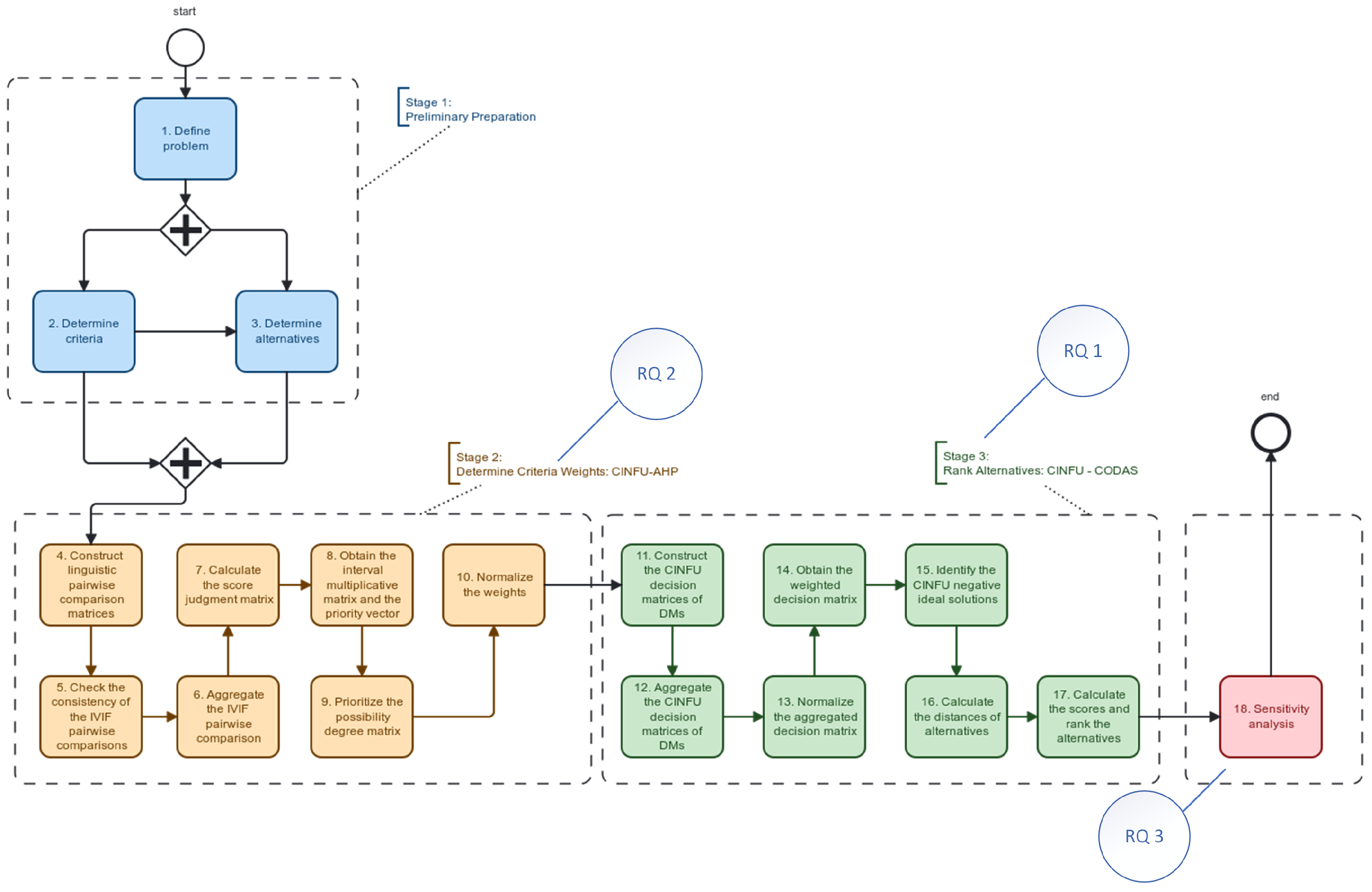
5.1. Stage 1: Preliminary Preparation

The CINFU AHP&CODAS methodology was applied to the machine selection problem for inventory tracking in a small and medium-sized manufacturing company working in the Turkish market. Deciding on a suitable machine is critical for a business in terms of accuracy, operational efficiency, cost savings, and continuity in inventory management. The criteria utilized in this study were established through a two-step process: a comprehensive literature review followed by expert consultations. The literature examined provided an initial set of potential criteria for machine selection in lean manufacturing environments, which included speed, setup time, operational flexibility, cost, and sustainability. This initial list was subsequently refined and validated during consultation sessions with three manufacturing professionals, each possessing over ten years of industry experience. The criteria selected for this study incorporate both theoretical perspectives and practical requirements, ensuring their relevance to the specific context of decision-making.

The six criteria for assessing the four machine options were derived. Each represents a particular facet of machine efficiency and compatibility with lean manufacturing and digital transformation objectives. Speed (C1) and Setup Time (C2) address operational efficiency. Ease to Operate and Move (C3) and Ability to Handle Multiple Operations (C4) evaluate flexibility and functionality. Maintenance and Energy Costs (C5) and Lifetime (C6) focus on long-term sustainability and cost-effectiveness.

Table 2. Criteria description.

Criterion	Description
Speed (C1)	Measures the machine’s inventory processing speed.
Setup Time (C2)	Time required to configure and initialize the machine.
Ease to Operate (C3)	Evaluates user-friendliness and mobility.
Multi-Operations (C4)	Assesses the machine’s ability to perform various tasks.
Maintenance Costs (C5)	Includes regular maintenance and energy consumption.
Lifetime (C6)	Expected operational lifespan of the machine.

gives the criteria definitions.

Various automated solutions offer distinct advantages tailored to different operational needs in inventory management. The High-Speed Automated Scanner (A1) provides sophisticated scanning capabilities for tracking inventory. It boasts state-of-the-art sensors and barcode reading technology, enabling rapid counting and logging of inventory with exceptional accuracy. Its compact structure is well suited for fast-paced manufacturing environments where space is at a premium. However, the substantial upfront investment and energy usage could influence its long-term economic viability.

The Multi-Functional Robotic Arm (A2) is designed for various inventory management functions, such as counting, sorting, and transferring materials. It highlights operational versatility, featuring programmable capabilities that allow it to cater to different types of inventory. Although it may be slower in purely counting tasks, its multifunctional abilities make it a valuable asset for intricate workflows.

The Mobile Inventory Tracker (A3) facilitates mobile inventory tracking, prioritizing user-friendliness and mobility across various production areas. With IoT connectivity, it seamlessly integrates into digital transformation efforts by delivering real-time updates on inventory status. Its portability and relatively low upkeep costs are notable benefits, although it may not be as efficient in large-scale operations as fixed systems.

The traditional counting machine, the Cost-Efficient Fixed Inventory Counter (A4), is designed for energy efficiency and robustness. It is optimized for managing high inventory volumes with minimal interruptions, making it ideal for more extensive operations. While it does not offer advanced features like IoT connectivity or multifunctionality, its lower initial and operational costs render it a practical choice for small and medium-sized businesses.

5.2. Stage 2: Determine Criteria Weights with CINFU-AHP

The experts were carefully selected to ensure they possessed relevant expertise in manufacturing systems, inventory management, and decision-making methodologies. Each expert has over 10 years of professional experience in fields pertinent to this study. Expert 1 is a senior production engineer specializing in lean manufacturing with extensive experience optimizing inventory workflows for small and medium-sized enterprises. Expert 2 is a manufacturing consultant strongly emphasizing integrating digital transformation technologies, including Internet of Things systems and machine optimization. Expert 3 is an academic specializing in multi-criteria decision-making and its applications in manufacturing and logistics. While we recognize the limited number of experts, we sought to maintain a balanced representation of academic and industry perspectives. The weights assigned to each expert reflect their experience and the relevance of their contributions to the study. To ensure the consistency of the expert evaluations, we employed the consistency ratio check for pairwise comparisons during the CINFU AHP process. All comparisons adhered to Saaty’s consistency threshold [41], ensuring the reliability of the input data.

The CINFU pairwise comparison matrices were collected during the experts’ meetings. The weights of the experts ($E1$, $E2$, and $E3$) were set to 0.30, 0.40, and 0.30, respectively, according to their experience. The experts evaluated the criteria using the CINFU linguistic scale presented in Table 1. The experts also chose two diverse $\zeta$ values between 0 and 1. Then, the CINFU pairwise comparison matrices were formed for each expert based on $\zeta$ values, as presented in

Table 3. CINFU linguistic pairwise comparison matrix with $\zeta$ values.

	Expert	C1	C2	C3	C4	C5	C6
C1	E1	EEI; (0.5, 0.5)	SlMI; (0.57, 0.63)	StMI; (0.35, 0.42)	SlMI; (0.3, 0.62)	SlMI; (0.4, 0.5)	StMI; (0.4, 0.5)
	E2	EEI; (0.5, 0.5)	SlMI; (0.52, 0.58)	StMI; (0.31, 0.47)	SlMI; (0.33, 0.47)	SlMI; (0.42, 0.47)	VSMI; (0.44, 0.67)
	E3	EEI; (0.5, 0.5)	StMI; (0.44, 0.51)	SlMI; (0.72, 0.78)	EEI; (0.44, 0.57)	SlMI; (0.35, 0.43)	SlMI; (0.55, 0.6)
C2	E1	SlLI; (0.4, 0.5)	StMI; (0.48, 0.57)	EEI; (0.33, 0.45)	SlLI; (0.4, 0.45)	EEI; (0.5, 0.5)	SlMI; (0.23, 0.28)
	E2	SlLI; (0.42, 0.47)	SlMI; (0.45, 0.52)	EEI; (0.28, 0.47)	SlLI; (0.21, 0.56)	EEI; (0.5, 0.5)	SlMI; (0.57, 0.77)
	E3	SlLI; (0.35, 0.43)	StMI; (0.43, 0.58)	SlMI; (0.39, 0.47)	StLI; (0.56, 0.65)	EEI; (0.5, 0.5)	SlMI; (0.34, 0.65)
C3	E1	StLI; (0.35, 0.42)	EEI; (0.23, 0.39)	EEI; (0.5, 0.5)	SlLI; (0.53, 0.58)	EEI; (0.33, 0.45)	EEI; (0.33, 0.67)
	E2	StLI; (0.31, 0.47)	SlMI; (0.31, 0.39)	EEI; (0.5, 0.5)	SlLI; (0.54, 0.56)	EEI; (0.28, 0.47)	EEI; (0.66, 0.76)
	E3	SlLI; (0.72, 0.78)	SlMI; (0.31, 0.43)	EEI; (0.5, 0.5)	StLI; (0.4, 0.48)	SlLI; (0.39, 0.47)	SlMI; (0.45, 0.48)
C4	E1	SlLI; (0.57, 0.63)	EEI; (0.5, 0.5)	EEI; (0.23, 0.39)	StLI; (0.24, 0.47)	StLI; (0.48, 0.57)	SlLI; (0.23, 0.56)
	E2	SlLI; (0.52, 0.58)	EEI; (0.5, 0.5)	SlLI; (0.31, 0.39)	StLI; (0.11, 0.34)	SlLI; (0.45, 0.52)	SlLI; (0.25, 0.35)
	E3	StLI; (044, 0.51)	EEI; (0.5, 0.5)	SlLI; (0.31, 0.43)	StLI; (0.25, 0.4)	StLI; (0.43, 0.58)	SlLI; (0.51, 0.77)
C5	E1	SlLI; (0.3, 0.62)	StMI; (0.24, 0.47)	SlMI; (0.53, 0.58)	EEI; (0.5, 0.5)	SlMI; (0.4, 0.45)	SlMI; (0.5, 0.63)
	E2	SlLI; (0.33, 0.47)	StMI; (0.11, 0.34)	SlMI; (0.54, 0.56)	EEI; (0.5, 0.5)	SlMI; (0.21, 0.56)	SlMI; (0.38, 0.43)
	E3	EEI; (0.44, 0.57)	StMI; (0.25, 0.4)	StMI; (0.4, 0.48)	EEI; (0.5, 0.5)	StMI; (0.56, 0.65)	StMI; (0.65, 0.8)
C6	E1	StLI; (0.4, 0.5)	SlMI; (0.23, 0.56)	EEI; (0.33, 0.67)	SlLI; (0.5, 0.63)	SlLI; (0.23, 0.28)	EEI; (0.5, 0.5)
	E2	VSLI; (0.44, 0.67)	SlMI; (0.25, 0.35)	EEI; (0.66, 0.76)	SlLI; (0.38, 0.43)	SlLI; (0.57, 0.77)	EEI; (0.5, 0.5)
	E3	SlLI; (0.55, 0.6)	SlMI; (0.51, 0.77)	SlLI; (0.45, 0.48)	StLI; (0.65, 0.8)	SlLI; (0.34, 0.65)	EEI; (0.5, 0.5)

. The linguistic evaluations were converted into related CINFUNs for each $\zeta$ value, as presented in

Table 4. Interval-valued intuitionistic fuzzy set pairwise comparison.

	Expert	C1	C2	C3	C4	C5	C6
C1	E1	([0.5, 0.5],	([0.583, 0.613],	([0.683, 0.731],	([0.525, 0.589],	([0.6, 0.625],	([0.72, 0.75],
		[0.5, 0.5])	[0.35, 0.368])	[0.228, 0.244])	[0.315, 0.353])	[0.36, 0.375])	[0.24, 0.25])
	E2	([0.5, 0.5],	([0.609, 0.624],	([0.642, 0.747],	([0.553, 0.623],	([0.609, 0.623],	([0.774, 0.862],
		[0.5, 0.5])	[0.365, 0.374])	[0.214, 0.249])	[0.332, 0.374])	[0.365, 0.374])	[0.111, 0.123])
	E3	([0.5, 0.5],	([0.739, 0.75],	([0.429, 0.504],	([0.49, 0.493],	([0.569, 0.613],	([0.6, 0.619],
		[0.5, 0.5])	[0.246, 0.25])	[0.257, 0.302])	[0.49, 0.493])	[0.341, 0.368])	[0.36, 0.371])
C2	E1	([0.36, 0.375],	([0.735, 0.749],	([0.442, 0.495],	([0.36, 0.371],	([0.5, 0.5],	([0.443, 0.504],
		[0.6, 0.625])	[0.245, 0.25])	[0.442, 0.495])	[0.6, 0.619])	[0.5, 0.5])	[0.266, 0.302])
	E2	([0.365, 0.374],	([0.619, 0.624],	([0.403, 0.498],	([0.249, 0.37],	([0.5, 0.5],	([0.443, 0.613],
		[0.609, 0.623])	[0.371, 0.374])	[0.403, 0.498])	[0.415, 0.616])	[0.5, 0.5])	[0.266, 0.368])
	E3	([0.341, 0.368],	([0.731, 0.735],	([0.595, 0.623],	([0.228, 0.246],	([0.5, 0.5],	([0.561, 0.569],
		[0.569, 0.613])	[0.244, 0.245])	[0.357, 0.374])	[0.683, 0.739])	[0.5, 0.5])	[0.337, 0.341])
C3	E1	([0.228, 0.244],	([0.354, 0.476],	([0.5, 0.5],	([0.365, 0.374],	([0.442, 0.495],	([0.442, 0.442],
		[0.683, 0.731])	[0.354, 0.476])	[0.5, 0.5])	[0.609, 0.623])	[0.442, 0.495])	[0.442, 0.442])
	E2	([0.214, 0.249],	([0.535, 0.595],	([0.5, 0.5],	([0.37, 0.373],	([0.403, 0.498],	([0.365, 0.449],
		[0.642, 0.747])	[0.321, 0.357])	[0.5, 0.5])	[0.616, 0.621])	[0.403, 0.498])	[0.365, 0.449])
	E3	([0.257, 0.302],	([0.535, 0.613],	([0.5, 0.5],	([0.24, 0.25],	([0.357, 0.374],	([0.619, 0.624],
		[0.429, 0.504])	[0.321, 0.368])	[0.5, 0.5])	[0.72, 0.749])	[0.595, 0.623])	[0.371, 0.374])
C4	E1	([0.35, 0.368],	([0.5, 0.5],	([0.354, 0.476],	([0.182, 0.249],	([0.245, 0.25],	([0.266, 0.37],
		[0.583, 0.613])	[0.5, 0.5])	[0.354, 0.476])	[0.547, 0.747])	[0.735, 0.749])	[0.443, 0.616])
	E2	([0.365, 0.374],	([0.5, 0.5],	([0.321, 0.357],	([0.098, 0.224],	([0.371, 0.374],	([0.281, 0.341],
		[0.609, 0.624])	[0.5, 0.5])	[0.535, 0.595])	[0.294, 0.673])	[0.619, 0.624])	[0.469, 0.569])
	E3	([0.246, 0.25],	([0.5, 0.5],	([0.321, 0.368],	([0.188, 0.24],	([0.244, 0.245],	([0.266, 0.375],
		[0.739, 0.75])	[0.5, 0.5])	[0.535, 0.613])	[0.563, 0.72])	[0.731, 0.735])	[0.443, 0.625])
C5	E1	([0.315, 0.353],	([0.547, 0.747],	([0.609, 0.623],	([0.5, 0.5],	([0.6, 0.619],	([0.583, 0.625],
		[0.525, 0.589])	[0.182, 0.249])	[0.365, 0.374])	[0.5, 0.5])	[0.36, 0.371])	[0.35, 0.375])
	E2	([0.332, 0.374],	([0.294, 0.673],	([0.616, 0.621],	([0.5, 0.5],	([0.415, 0.616],	([0.589, 0.613],
		[0.553, 0.623])	[0.098, 0.224])	[0.37, 0.373])	[0.5, 0.5])	[0.249, 0.37])	[0.353, 0.368])
	E3	([0.49, 0.493],	([0.563, 0.72],	([0.72, 0.749],	([0.5, 0.5],	([0.683, 0.739],	([0.48, 0.683],
		[0.49, 0.493])	[0.188, 0.24])	[0.24, 0.25])	[0.5, 0.5])	[0.228, 0.246])	[0.16, 0.228])
C6	E1	([0.24, 0.25],	([0.443, 0.616],	([0.442, 0.442],	([0.35, 0.375],	([0.266, 0.302],	([0.5, 0.5],
		[0.72, 0.75])	[0.266, 0.37])	[0.442, 0.442])	[0.583, 0.625])	[0.443, 0.504])	[0.5, 0.5])
	E2	([0.111, 0.123],	([0.469, 0.569],	([0.365, 0.449],	([0.353, 0.368],	([0.266, 0.368],	([0.5, 0.5],
		[0.774, 0.862])	[0.281, 0.341])	[0.365, 0.449])	[0.589, 0.613])	[0.443, 0.613])	[0.5, 0.5])
	E3	([0.36, 0.371],	([0.443, 0.625],	([0.371, 0.374],	([0.16, 0.228],	([0.337, 0.341],	([0.5, 0.5],
		[0.6, 0.619])	[0.266, 0.375])	[0.619, 0.624])	[0.48, 0.683])	[0.561, 0.569])	[0.5, 0.5])

.

For an example calculation of Table 4, the bold IVIF number ([0.683, 0.731], [0.228, 0.244]) in C1–C3 for Expert 1 is shown here. Expert 1 evaluated StMI with the two $\zeta$ values as 0.35 and 0.42 when comparing C1–C3, as presented in Table 3. ${\mu }_1=3\zeta -3{\zeta }^2=3\times 0.35-3\times 0.{35}^2=0.683$ for the $\zeta =0.35$ and ${\mu }_2=1\zeta -1{\zeta }^2=1\times 0.42-1\times 0.{42}^2=0.731$ for $\zeta =0.35$. A similar calculation for non-membership values $({\upsilon }_1,{\upsilon }_2)$ was implemented. Each IVIF pairwise comparison judgment was defuzzified for each expert by using Equation (13). Then, the consistency ratios were computed.

Table 5. Aggregated IVIF pairwise comparison matrix.

	C1	C2	C3	C4	C5	C6
C1	([0.5, 0.5],	([0.595, 0.62],	([0.603, 0.685],	([0.647, 0.664],	([0.526, 0.577],	([0.714,0.777],
	[0.5, 0.5])	[0.356,0.372])	[0.23, 0.262])	[0.32, 0.33])	[0.367, 0.399])	[0.199, 0.212])
C2	([0.357, 0.372],	([0.5, 0.5],	([0.479,0.538],	([0.692, 0.7],	([0.278, 0.335],	([0.481, 0.569],
	[0.594, 0.62])	[0.5, 0.5])	[0.4, 0.456])	[0.289, 0.292])	[0.538, 0.652])	[0.285, 0.339])
C3	([0.231, 0.264],	([0.402, 0.463],	([0.5, 0.5],	([0.487, 0.568],	([0.332, 0.338],	([0.476, 0.507],
	[0.579, 0.66])	[0.466, 0.532])	[0.5, 0.5])	[0.331, 0.393])	[0.643, 0.657])	[0.389, 0.423])
C4	([0.327, 0.337],	([0.298, 0.301],	([0.331, 0.398],	([0.5, 0.5],	([0.151, 0.237],	([0.272, 0.36],
	[0.637, 0.656])	[0.685, 0.692])	[0.473, 0.561])	[0.5, 0.5])	[0.43, 0.709])	[0.453, 0.599])
C5	([0.379, 0.406],	([0.565, 0.659],	([0.649, 0.665],	([0.465, 0.711],	([0.5, 0.5],	([0.557,0.639],
	[0.525, 0.571])	[0.271, 0.328])	[0.324, 0.331])	[0.143, 0.236])	[0.5, 0.5])	[0.278, 0.32])
C6	([0.231, 0.243],	([0.288, 0.341],	([0.391, 0.425],	([0.453, 0.601],	([0.299, 0.331],	([0.5, 0.5],
	[0.702, 0.749])	[0.475, 0.565])	[0.453, 0.493])	[0.272, 0.36])	[0.552, 0.637])	[0.5, 0.5])

indicates the aggregated IVIF pairwise comparison matrix. Because pairwise comparisons were made by three experts with different weights (0.30, 0.40, and 0.30 for E1, E2, and E3, respectively), the methodology aggregates the IVIF pairwise comparison matrices using the IVIFWG operator given in Equation (20).

Some interesting results were obtained after aggregating the experts’ comparisons. The IVIFN for Speed (C1) vs. Lifetime (C6) is ([0.714, 0.777], [0.199, 0.212]), indicating a strong consensus among the experts that Speed is immensely more important than Lifetime in this particular decision context. The membership interval suggests a high degree of certainty in this judgment.

The IVIFN for Setup Time (C2) vs. Ability to Handle Multiple Operations (C4) is ([0.692, 0.7], [0.289, 0.292]). This comparison is particularly interesting because it exposes a close contest between Setup Time and the machine’s versatility. While the membership interval slightly favors Setup Time, the narrow range and the relatively high non-membership values suggest that experts are somewhat divided on the matter.

The IVIFN for Ease to Operate and Move (C3) vs. Maintenance and Energy Cost (C5) is ([0.332, 0.338], [0.643, 0.657]). In contrast to the previous examples, this comparison shows an obvious choice for Maintenance and Energy Costs over Ease of Operation and Movement. The low membership and high non-membership values show a powerful consensus among the experts on this comparison.

Table 6. Score judgment matrix.

	C1	C2	C3	C4	C5	C6
C1	(0, 0)	(0.222, 0.264)	(0.34, 0.454)	(0.317, 0.344)	(0.127, 0.21)	(0.502, 0.578)
C2	(−0.264, −0.222)	(0, 0)	(0.023, 0.139)	(0.4, 0.411)	(−0.373, −0.203)	(0.142, 0.284)
C3	(−0.428, −0.315)	(−0.13, −0.003)	(0, 0)	(0.094, 0.238)	(−0.326, −0.305)	(0.053, 0.118)
C4	(−0.329, −0.3)	(−0.394, −0.384)	(−0.23, −0.074)	(0, 0)	(−0.558, −0.194)	(−0.327, −0.093)
C5	(−0.192, −0.119)	(0.238, 0.388)	(0.318, 0.342)	(0.228, 0.568)	(0, 0)	(0.237, 0.361)
C6	(−0.517, −0.459)	(−0.277, −0.135)	(−0.102, −0.027)	(0.094, 0.329)	(−0.337, −0.221)	(0, 0)

gives the score judgment matrix from the aggregated IVIF pairwise comparison matrix formed (Table 5) using Equation (23). The score judgment matrix transforms the IVIFNs into a more straightforward numerical form that can be used for further analysis in the CINFU AHP method. The converted numerical form consists of an interval indicating the general preference for one criterion over another, considering the IVIFN’s membership and non-membership degrees.

A wider interval implies more uncertainty in the comparison, while a narrower interval reveals a higher degree of consensus. A positive score in the interval suggests that the criterion in the row is preferred over the criterion in the column. Conversely, a negative score in the interval indicates the opposite. The comparison becomes imprecise if the interval spans zero, suggesting no clear preference.

After calculating the score judgment matrix, some interesting criteria comparisons were given. The score interval for Speed (C1) vs. Setup Time (C2), (0.222, 0.264) has a positive interval and apparently shows Speed is more important than Setup Time. The narrow range denotes a relatively strong consensus among the experts regarding this preference.

The score interval for Setup Time (C2) vs. Ease to Operate and Move (C3), (0.023, 0.139) is positive, albeit it is a narrow one and close to zero, implying a slight preference for Setup Time over Ease of Operation and Move. The closeness to zero and the narrow range present a marginal preference and a potential area where expert opinions might be more divergent.

The score interval for Ability to Handle Multiple Operations (C4) vs. Lifetime (C6) is (−0.327, −0.093). This negative score interval demonstrates that Lifetime was considered more important than Ability to Handle Multiple Operations. This preference might reflect a long-term focus where the machine’s durability is prioritized over its versatility.

Table 7. Interval multiplicative matrix.

	C1	C2	C3	C4	C5	C6
C1	(1, 1)	(1.666, 1.836)	(2.19, 2.847)	(1.99, 2.207)	(1.32, 1.555)	(3.175, 3.782)
C2	(0.545, 0.6)	(1, 1)	(1.055, 1.348)	(2.421, 2.578)	(0.409, 0.578)	(1.387, 1.923)
C3	(0.373, 0.484)	(0.726, 0.948)	(1, 1)	(1.187, 1.728)	(0.455, 0.481)	(1.129, 1.313)
C4	(0.469, 0.502)	(0.388, 0.398)	(0.589, 0.805)	(1, 1)	(0.271, 0.591)	(0.471, 0.807)
C5	(0.643, 0.761)	(1.594, 2.363)	(2.08, 2.116)	(1.562, 3.696)	(1, 1)	(1.725, 2.296)
C6	(0.304, 0.348)	(0.520, 0.721)	(0.79, 0.886)	(1.239, 2.124)	(0.436, 0.601)	(1, 1)

presents the interval multiplicative matrix calculated based on Table 6 using Equation (24), which involves transforming the score intervals into their corresponding multiplicative equivalents. The main purpose is to construct a comparable scale reflecting the strength of preference between criteria based on the score judgment matrix. Instead of direct score intervals, the multiplicative matrix emphasizes the factor by which one criterion is considered more important than another. This modification helps capture the preferences’ magnitude more effectively and enables the calculation of interval weights for the criteria.

If the interval in a cell has values greater than 1, it implies that the criterion in the row is regarded as more significant than the criterion in the column. The larger the values, the stronger the preference. Conversely, if the interval values are less than 1, the criterion in the column is preferred over the criterion in the row. Values closer to zero indicate a stronger preference. If the interval includes the value 1, it suggests an imprecise comparison with no clear choice between the two criteria.

After forming the interval multiplicative matrix, some interesting criteria comparisons were given. For criteria C1 (Speed) vs. C2 (Setup Time), the interval is (1.666, 1.836). This interval, with values greater than 1, reinforces that Speed is more important than Setup Time. The magnitude of the values means that Speed is considered approximately 1.7 times more critical than Setup Time.

The interval of C2 (Setup Time) vs. C3 (Ease to Operate and Move), (1.055, 1.348), has values greater than 1, showing a weak tendency for Setup Time over Ease of Operation because the values are positive but closer to 1.

With values less than 1, the interval multiplicative score for C4 (Ability to Handle Multiple Operations) vs. C6 (Lifetime) (0.471, 0.807) indicates that Lifetime is more critical than Ability to Handle Multiple Operations. Values closer to zero indicate a relatively strong preference for Lifetime.

Table 8. Priority vector.

Criterion	Interval
C1	(0.229, 0.330)
C2	(0.140, 0.206)
C3	(0.099, 0.152)
C4	(0.066, 0.106)
C5	(0.176, 0.313)
C6	(0.088, 0.147)

shows the priority vector, calculating the interval ${\tilde{\omega }}_j$ of the criteria based on Table 7 by utilizing Equation (25). This equation aggregates the multiplicative relationships produced from the interval multiplicative matrix (Table 7) to calculate the interval weights for each criterion.

Table 9. Possibility degree matrix.

	C1	C2	C3	C4	C5	C6
C1	-	1	1	1	0.649	1
C2	0	-	0.897	1	0.148	0.944
C3	0	0.103	-	0.926	0	0.576
C4	0	0	0.074	-	0	0.186
C5	0.351	0.852	1	1	-	1
C6	0	0.056	0.424	0.814	0	-

gives the possibility degree matrix obtained by comparing the priority vector for each criterion based on Table 8 using Equation (26). This matrix seeks to determine the possible overlapping and uncertainty inherent in the interval weights. For example, the priority vector for criterion C1 (Speed) is (0.229, 0.330). This interval indicates that the weight assigned to Speed in the machine selection process could fall between 0.229 and 0.330. For instance, the cell corresponding to C1 (Speed) and C2 (Setup Time) with a value of 1 suggests that Speed can be considered to be 100% more important than Setup Time based on the priority vectors.

Then, the prioritized possibility degrees were originated by employing Equation (27), and the normalized criteria weights were obtained by Equation (28), which yields the crisp numerical weights to each criterion from the possibility degree matrix, as shown in

Table 10. Normalized criteria weights.

Criterion	Weight
C1	0.25
C2	0.08
C3	0.13
C4	0.23
C5	0.18
C6	0.12

. For example, the normalized weight for C1 (Speed) is 0.25, which indicates that Speed has a 25% weight in the overall machine selection decision.

5.3. Stage 3: Rank Alternatives with CINFU-CODAS

After computing the criteria weights with the CINFU AHP method, the alternatives based on the criteria set were then evaluated using the CINFU CODAS technique. The experts evaluated the alternatives with respect to each criterion using the linguistic evaluation in

Table 11. Linguistic decision matrices for alternatives.

		A1	A2	A3	A4
C1	E1	HV	VHV	SHV	MV
	E2	VHV	VHV	SHV	MV
	E3	MV	SHV	VHV	HV
C2	E1	VHV	HV	SHV	MV
	E2	VHV	HV	SHV	MV
	E3	VHV	HV	SHV	MV
C3	E1	HV	HV	VHV	VHV
	E2	SHV	SHV	HV	VHV
	E3	SHV	SHV	HV	VHV
C4	E1	SHV	HV	VHV	VHV
	E2	SHV	HV	HV	VHV
	E3	SHV	SHV	HV	VHV
C5	E1	VHV	HV	SHV	MV
	E2	VHV	HV	SHV	MV
	E3	VHV	HV	SHV	MV
C6	E1	MV	SHV	HV	VHV
	E2	SHV	HV	HV	VHV
	E3	SHV	HV	VHV	VHV

. The cost criteria C2 and C5 were transformed into benefit criteria at the beginning of the analysis.

Table 1 transforms the linguistic judgments into their CINFU values. The aggregated normalized CINFU matrix, shown in

Table 12. Aggregated normalized CINFU decision matrix.

		A1		A2		A3		A4
	$\mathit{\zeta }$	$\mathit{\mu }$	$\mathit{\upsilon }$	$\mathit{\mu }$	$\mathit{\upsilon }$	$\mathit{\mu }$	$\mathit{\upsilon }$	$\mathit{\mu }$	$\mathit{\upsilon }$
C1	0.1	0.254	0.101	0.285	0.073	0.249	0.109	0.203	0.154
	0.2	0.452	0.182	0.506	0.131	0.442	0.195	0.361	0.275
	0.3	0.593	0.243	0.664	0.174	0.581	0.258	0.474	0.364
	0.4	0.678	0.281	0.759	0.2	0.664	0.296	0.542	0.417
	0.5	0.706	0.294	0.791	0.209	0.691	0.309	0.565	0.435
	0.6	0.678	0.281	0.759	0.2	0.664	0.296	0.542	0.417
	0.7	0.593	0.243	0.664	0.174	0.581	0.258	0.474	0.364
	0.8	0.452	0.182	0.506	0.131	0.442	0.195	0.361	0.275
	0.9	0.254	0.101	0.285	0.073	0.249	0.109	0.203	0.154
C2	0.1	0.315	0.045	0.27	0.09	0.225	0.135	0.18	0.18
	0.2	0.56	0.08	0.48	0.16	0.4	0.24	0.32	0.32
	0.3	0.735	0.105	0.63	0.21	0.525	0.315	0.42	0.42
	0.4	0.84	0.12	0.72	0.24	0.6	0.36	0.48	0.48
	0.5	0.875	0.125	0.75	0.25	0.625	0.375	0.5	0.5
	0.6	0.84	0.12	0.72	0.24	0.6	0.36	0.48	0.48
	0.7	0.735	0.105	0.63	0.21	0.525	0.315	0.42	0.42
	0.8	0.56	0.08	0.48	0.16	0.4	0.24	0.32	0.32
	0.9	0.315	0.045	0.27	0.09	0.225	0.135	0.18	0.18
C3	0.1	0.238	0.122	0.238	0.122	0.283	0.077	0.315	0.045
	0.2	0.422	0.217	0.422	0.217	0.503	0.137	0.56	0.08
	0.3	0.555	0.285	0.555	0.285	0.66	0.18	0.735	0.105
	0.4	0.634	0.326	0.634	0.326	0.754	0.206	0.84	0.12
	0.5	0.66	0.34	0.66	0.34	0.785	0.215	0.875	0.125
	0.6	0.634	0.326	0.634	0.326	0.754	0.206	0.84	0.12
	0.7	0.555	0.285	0.555	0.285	0.66	0.18	0.735	0.105
	0.8	0.422	0.217	0.422	0.217	0.503	0.137	0.56	0.08
	0.9	0.238	0.122	0.238	0.122	0.283	0.077	0.315	0.045
C4	0.1	0.225	0.135	0.256	0.104	0.283	0.077	0.315	0.045
	0.2	0.4	0.24	0.454	0.185	0.503	0.137	0.56	0.08
	0.3	0.525	0.315	0.596	0.243	0.66	0.18	0.735	0.105
	0.4	0.6	0.36	0.682	0.278	0.754	0.206	0.84	0.12
	0.5	0.625	0.375	0.71	0.29	0.785	0.215	0.875	0.125
	0.6	0.6	0.36	0.682	0.278	0.754	0.206	0.84	0.12
	0.7	0.525	0.315	0.596	0.243	0.66	0.18	0.735	0.105
	0.8	0.4	0.24	0.454	0.185	0.503	0.137	0.56	0.08
	0.9	0.225	0.135	0.256	0.104	0.283	0.077	0.315	0.045
C5	0.1	0.315	0.045	0.27	0.09	0.225	0.135	0.18	0.18
	0.2	0.56	0.08	0.48	0.16	0.4	0.24	0.32	0.32
	0.3	0.735	0.105	0.63	0.21	0.525	0.315	0.42	0.42
	0.4	0.84	0.12	0.72	0.24	0.6	0.36	0.48	0.48
	0.5	0.875	0.125	0.75	0.25	0.625	0.375	0.5	0.5
	0.6	0.84	0.12	0.72	0.24	0.6	0.36	0.48	0.48
	0.7	0.735	0.105	0.63	0.21	0.525	0.315	0.42	0.42
	0.8	0.56	0.08	0.48	0.16	0.4	0.24	0.32	0.32
	0.9	0.315	0.045	0.27	0.09	0.225	0.135	0.18	0.18
C6	0.1	0.21	0.149	0.256	0.104	0.283	0.077	0.315	0.045
	0.2	0.374	0.265	0.454	0.185	0.503	0.137	0.56	0.08
	0.3	0.491	0.348	0.596	0.243	0.66	0.18	0.735	0.105
	0.4	0.561	0.399	0.682	0.278	0.754	0.206	0.84	0.12
	0.5	0.585	0.415	0.71	0.29	0.785	0.215	0.875	0.125
	0.6	0.561	0.399	0.682	0.278	0.754	0.206	0.84	0.12
	0.7	0.491	0.348	0.596	0.243	0.66	0.18	0.735	0.105
	0.8	0.374	0.265	0.454	0.185	0.503	0.137	0.56	0.08
	0.9	0.21	0.149	0.256	0.104	0.283	0.077	0.315	0.045

, was acquired employing the CINFUWG operator given in Equation (20). This matrix connects the expert preferences of each alternative machine across various criteria and alters them into a comparative form for further analysis. The alternatives and criteria are located in the rows and columns, respectively, and the aggregated and normalized CINFUNs, described by their membership ($\mu$) and non-membership ($\upsilon$) degrees for various $\zeta$ values, expressing the ‘optimism level’ of the expert, are given in the intersections. For example, in the evaluation of alternative A1 with respect to the criterion C1 (Speed) at $\zeta$ = 0.5, the aggregated normalized CINFUN, $\mu =0.706$, $\upsilon =0.294$, reveals a strongly positive assessment of A1’s speed, with a high membership degree (0.706), denoting a powerful consensus among experts that A1 performs well on this criterion. The relatively low non-membership degree (0.294) supports this positive view, presenting little conflict or uncertainty.

Then, the weighted normalized CINFU decision matrix was formed from the weights obtained from CINFU AHP. Multiplying the normalized CINFUNs with their respective weights guarantees that criteria with higher weights are a high proportion, showing a more significant influence on the final ranking.

The CINFU negative ideal solution (NIS CINFU) represents a theoretical machine that is the worst alternative for all criteria. It was determined by specifying the minimum score values among the weighted normalized alternative evaluations for each criterion using Equation (33) in

Table 13. Weighted normalized CINFU decision matrix.

Criterion	$\mathit{\zeta }$	A1		A2		A3		A4		Negative Ideal Solution
		$\mathit{\mu }$	$\mathit{\upsilon }$	$\mathit{\mu }$	$\mathit{\upsilon }$	$\mathit{\mu }$	$\mathit{\upsilon }$	$\mathit{\mu }$	$\mathit{\upsilon }$	$\mathit{\mu }$	$\mathit{\upsilon }$
C1	0.1	0.07	0.568	0.079	0.525	0.068	0.579	0.054	0.631	0.054	0.631
	0.2	0.138	0.658	0.16	0.607	0.134	0.669	0.105	0.728	0.105	0.728
	0.3	0.199	0.706	0.236	0.65	0.193	0.716	0.146	0.78	0.146	0.78
	0.4	0.244	0.731	0.296	0.673	0.235	0.741	0.175	0.806	0.175	0.806
	0.5	0.26	0.74	0.32	0.68	0.251	0.749	0.185	0.815	0.185	0.815
	0.6	0.244	0.731	0.296	0.673	0.235	0.741	0.175	0.806	0.175	0.806
	0.7	0.199	0.706	0.236	0.65	0.193	0.716	0.146	0.78	0.146	0.78
	0.8	0.138	0.658	0.16	0.607	0.134	0.669	0.105	0.728	0.105	0.728
	0.9	0.07	0.568	0.079	0.525	0.068	0.579	0.054	0.631	0.054	0.631
C2	0.1	0.068	0.564	0.057	0.641	0.046	0.691	0.036	0.728	0.036	0.728
	0.2	0.141	0.627	0.114	0.713	0.09	0.768	0.069	0.81	0.069	0.81
	0.3	0.218	0.659	0.168	0.749	0.129	0.808	0.096	0.852	0.096	0.852
	0.4	0.287	0.676	0.21	0.768	0.156	0.828	0.114	0.873	0.114	0.873
	0.5	0.319	0.681	0.226	0.774	0.166	0.834	0.12	0.88	0.12	0.88
	0.6	0.287	0.676	0.21	0.768	0.156	0.828	0.114	0.873	0.114	0.873
	0.7	0.218	0.659	0.168	0.749	0.129	0.808	0.096	0.852	0.096	0.852
	0.8	0.141	0.627	0.114	0.713	0.09	0.768	0.069	0.81	0.069	0.81
	0.9	0.068	0.564	0.057	0.641	0.046	0.691	0.036	0.728	0.036	0.728
C3	0.1	0.036	0.755	0.036	0.755	0.043	0.71	0.049	0.661	0.036	0.755
	0.2	0.071	0.815	0.071	0.815	0.089	0.767	0.104	0.714	0.071	0.815
	0.3	0.102	0.846	0.102	0.846	0.134	0.795	0.162	0.74	0.102	0.846
	0.4	0.126	0.861	0.126	0.861	0.171	0.81	0.217	0.753	0.126	0.861
	0.5	0.134	0.866	0.134	0.866	0.186	0.814	0.242	0.758	0.134	0.866
	0.6	0.126	0.861	0.126	0.861	0.171	0.81	0.217	0.753	0.126	0.861
	0.7	0.102	0.846	0.102	0.846	0.134	0.795	0.162	0.74	0.102	0.846
	0.8	0.071	0.815	0.071	0.815	0.089	0.767	0.104	0.714	0.071	0.815
	0.9	0.036	0.755	0.036	0.755	0.043	0.71	0.049	0.661	0.036	0.755
C4	0.1	0.021	0.846	0.024	0.827	0.027	0.807	0.031	0.771	0.021	0.846
	0.2	0.042	0.887	0.049	0.868	0.057	0.847	0.066	0.809	0.042	0.887
	0.3	0.06	0.908	0.073	0.888	0.086	0.866	0.105	0.828	0.06	0.908
	0.4	0.074	0.918	0.091	0.898	0.111	0.876	0.142	0.837	0.074	0.918
	0.5	0.079	0.921	0.098	0.902	0.121	0.879	0.16	0.84	0.079	0.921
	0.6	0.074	0.918	0.091	0.898	0.111	0.876	0.142	0.837	0.074	0.918
	0.7	0.06	0.908	0.073	0.888	0.086	0.866	0.105	0.828	0.06	0.908
	0.8	0.042	0.887	0.049	0.868	0.057	0.847	0.066	0.809	0.042	0.887
	0.9	0.021	0.846	0.024	0.827	0.027	0.807	0.031	0.771	0.021	0.846
C5	0.1	0.083	0.49	0.07	0.575	0.057	0.631	0.045	0.674	0.045	0.674
	0.2	0.172	0.56	0.139	0.656	0.111	0.72	0.085	0.77	0.085	0.77
	0.3	0.263	0.596	0.204	0.699	0.157	0.767	0.118	0.819	0.118	0.819
	0.4	0.344	0.614	0.254	0.72	0.19	0.791	0.139	0.845	0.139	0.845
	0.5	0.38	0.62	0.273	0.727	0.202	0.798	0.147	0.853	0.147	0.853
	0.6	0.344	0.614	0.254	0.72	0.19	0.791	0.139	0.845	0.139	0.845
	0.7	0.263	0.596	0.204	0.699	0.157	0.767	0.118	0.819	0.118	0.819
	0.8	0.172	0.56	0.139	0.656	0.111	0.72	0.085	0.77	0.085	0.77
	0.9	0.083	0.49	0.07	0.575	0.057	0.631	0.045	0.674	0.045	0.674
C6	0.1	0.028	0.793	0.035	0.759	0.04	0.732	0.045	0.686	0.028	0.793
	0.2	0.056	0.85	0.071	0.814	0.082	0.785	0.095	0.735	0.056	0.85
	0.3	0.079	0.879	0.105	0.842	0.123	0.811	0.15	0.76	0.079	0.879
	0.4	0.096	0.894	0.13	0.855	0.157	0.825	0.2	0.772	0.096	0.894
	0.5	0.102	0.898	0.14	0.86	0.171	0.829	0.224	0.776	0.102	0.898
	0.6	0.096	0.894	0.13	0.855	0.157	0.825	0.2	0.772	0.096	0.894
	0.7	0.079	0.879	0.105	0.842	0.123	0.811	0.15	0.76	0.079	0.879
	0.8	0.056	0.85	0.071	0.814	0.082	0.785	0.095	0.735	0.056	0.85
	0.9	0.028	0.793	0.035	0.759	0.04	0.731	0.045	0.685	0.028	0.793

. For criterion C1 (Speed) at $\zeta =0.3$, the NIS CINFU is ($\mu =0.146$, $\upsilon =0.78$). This signifies that the worst possible performance in the Speed criterion would have a very low membership degree (0.146) and a very high non-membership degree (0.78), indicating a strong consensus that a machine with such an evaluation would be highly undesirable.

Table 14. Euclidean and Taxicab distances of alternatives.

	A1		A2		A3		A4
$\mathit{\zeta }$	Euclidean	Taxicab	Euclidean	Taxicab	Euclidean	Taxicab	Euclidean	Taxicab
0.1	0.095	0.069	0.064	0.058	0.043	0.046	0.061	0.046
0.2	0.103	0.077	0.07	0.065	0.045	0.051	0.062	0.049
0.3	0.11	0.082	0.076	0.068	0.048	0.053	0.063	0.051
0.4	0.123	0.084	0.084	0.07	0.053	0.055	0.069	0.052
0.5	0.131	0.084	0.088	0.071	0.056	0.055	0.074	0.052
0.6	0.123	0.084	0.084	0.07	0.053	0.055	0.069	0.052
0.7	0.11	0.082	0.076	0.068	0.048	0.053	0.063	0.051
0.8	0.103	0.077	0.07	0.065	0.045	0.051	0.062	0.049
0.9	0.095	0.069	0.064	0.058	0.043	0.046	0.061	0.046

shows the Taxicab and Euclidean distances of the alternatives of the CINFU negative ideal solution calculated by Equations (34) and (35). A shorter distance, whether Euclidean or Taxicab, implies that the alternative machine is nearer to the ideal solution and away from the NIS, meaning a better overall performance. Experts can evaluate their relative performance by comparing the distances of different alternatives. The expert’s optimism level $\zeta$ is a crucial factor significantly affecting the computed distances. A higher $\zeta$ value might result in larger distances, representing a more pessimistic perspective where dissimilarities from the ideal solution are strengthened. For example, at $\zeta =0.5$, alternative A1 and A3 have Euclidean distances of 0.131 and 0.056, respectively, and Taxicab distances of 0.084 and 0.055, respectively. These distances imply that A3 is closer to the ideal solution than A1. In other words, A3 is a more advantageous alternative at this particular $\zeta$ value.

Table 15. Alternative ranking.

$\mathit{\zeta }$	A1		A2		A3		A4
	Score	Ranking	Score	Ranking	Score	Ranking	Score	Ranking
0.1	0.173	1	−0.007	2	−0.126	4	−0.041	3
0.2	0.199	1	0.0003	2	−0.14	4	−0.059	3
0.3	0.217	1	0.007	2	−0.149	4	−0.075	3
0.4	0.237	1	0.009	2	−0.162	4	−0.084	3
0.5	0.249	1	0.007	2	−0.171	4	−0.084	3
0.6	0.237	1	0.009	2	−0.162	4	−0.084	3
0.7	0.217	1	0.007	2	−0.149	4	−0.075	3
0.8	0.199	1	0.0003	2	−0.14	4	−0.059	3
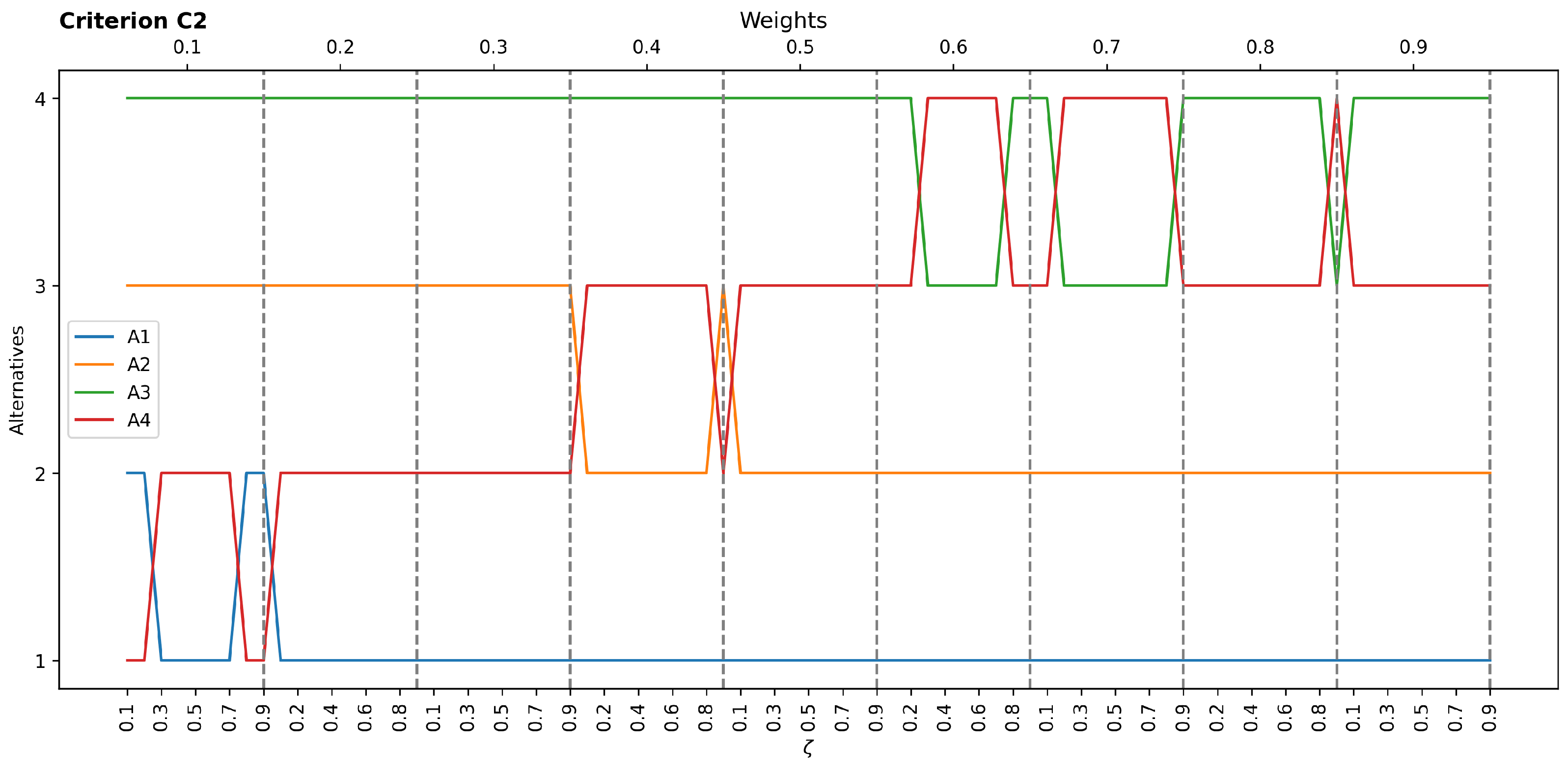
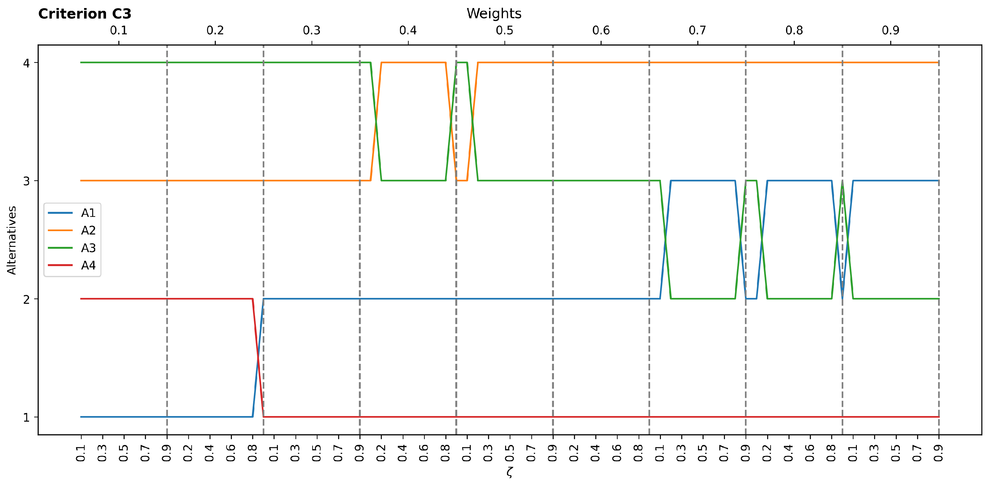
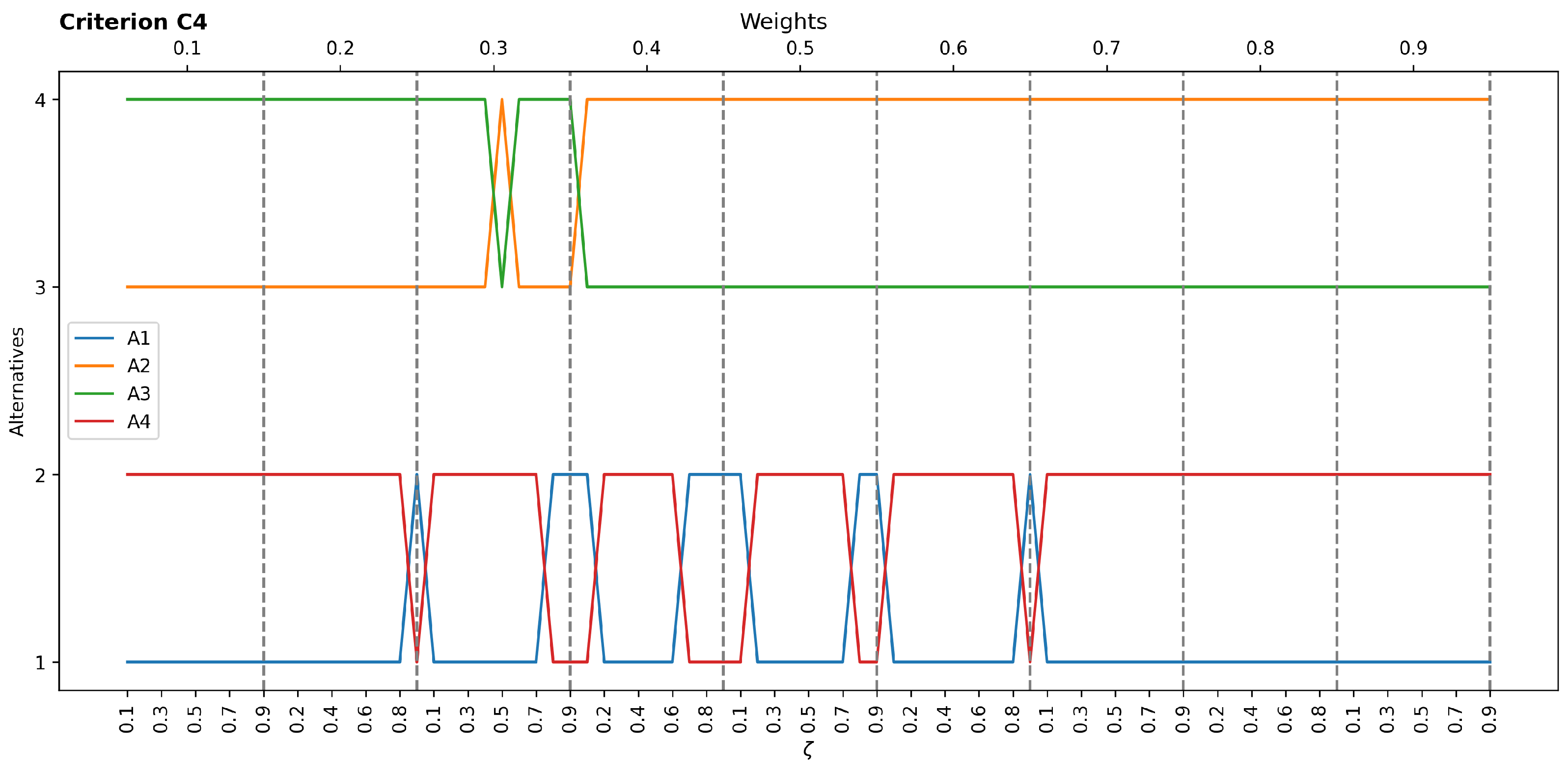
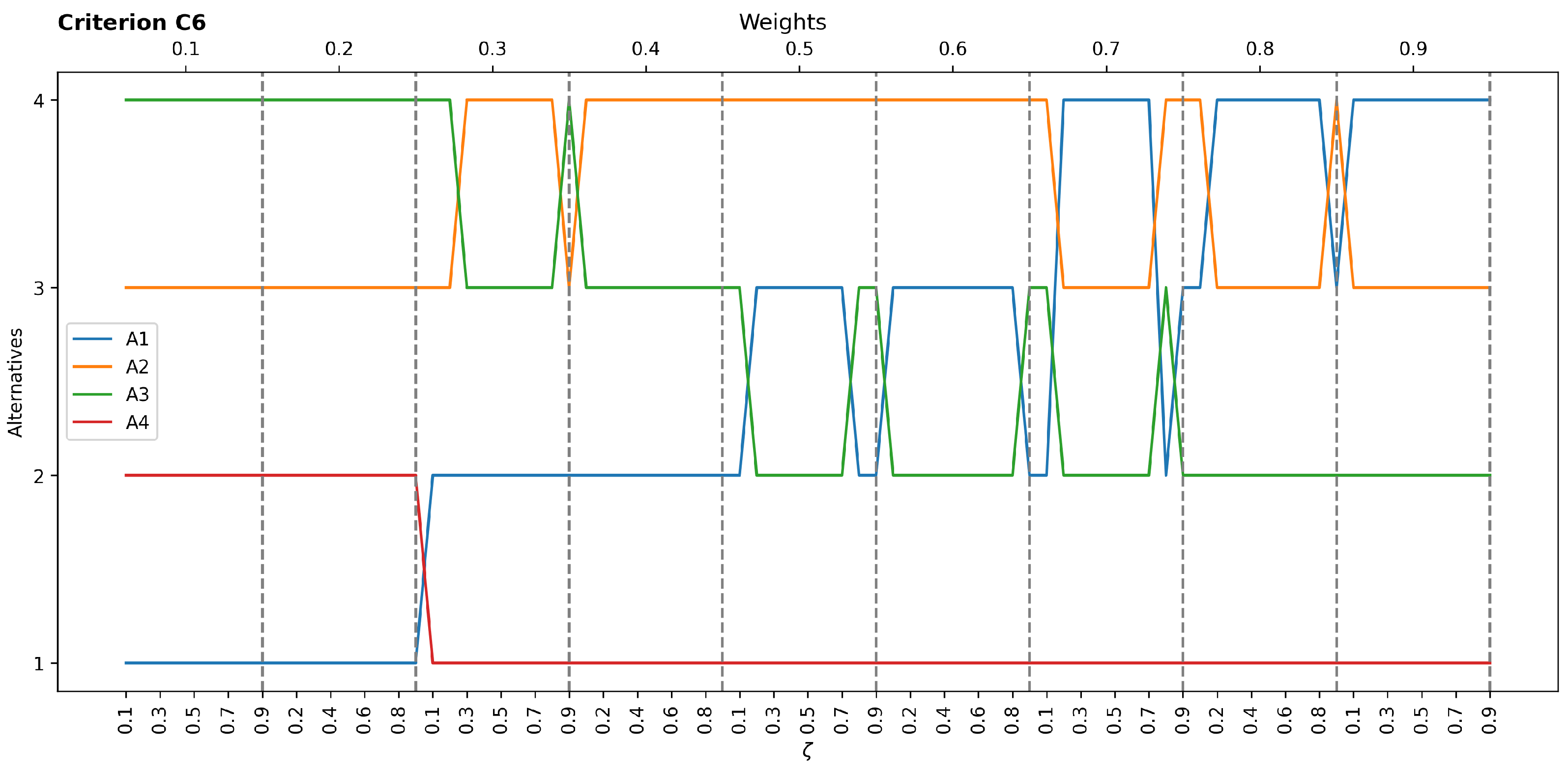
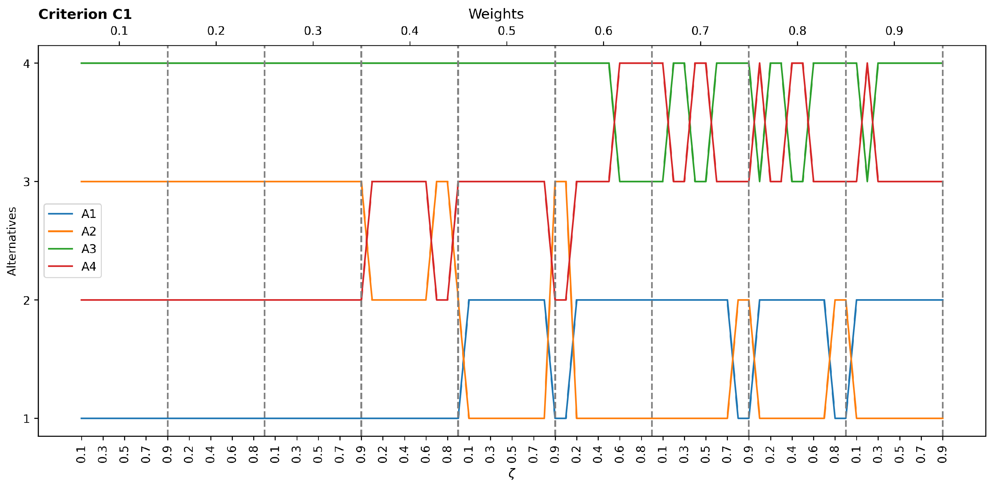
0.9	0.173	1	−0.007	2	−0.126	4	−0.041	3

indicates the alternatives’ assessment scores and ranking. A higher evaluation score means a better general performance and a more outstanding choice for a particular machine. The machines were ranked in descending order based on their evaluation scores.

Including multiple $\zeta$ values shows the potential impact of the expert’s optimism level on the final ranking. For example, at $\zeta =0.4$, A1 was placed as the most preferred machine with the highest score of 0.237. A3 was the least preferred choice, with the lowest score of −0.162. A2 and A4 fell in between, with A2 being more promising than A4 due to its higher score.

Although the $\zeta$ value may affect the ranking, in this application, the alternative ranking stays relatively consistent for different $\zeta$ values, presenting a robust and reliable outcome. The best machine for inventory tracking was A1, whereas the least desired one was A3 for any $\zeta$ values.

6. Sensitivity Analysis

The sensitivity results depict how changing the weight of a particular criterion affects the ranking of the alternative machines A1, A2, A3, and A4. One-at-a-time sensitivity analysis was used to specify how the output of the decision model (in this study, alternative rankings) varied as each input parameter (in this study, criterion weight) was changed separately, keeping all other parameters fixed at their baseline values. This type of analysis helps to understand the sensitivity of the output to each parameter in isolation and pinpoints which parameters have the most powerful impact on the decision model’s outcome.

A sensitivity analysis involving 81 different scenarios was performed to determine the impact of each criterion’s weight and $\zeta$ level changes on the final scores and ranking results of the alternatives. In each scenario, the criterion’s weight was increased from 0.1 to 0.9. While the weight of each criterion was changed, the weights of the remaining criteria were proportionally organized.

Figure 2 illustrates the sensitivity results concerning criterion C1 (Speed). A1 was placed in the first rank until the weight of C1 was below 0.5. When the weight of C1 is below 0.4, A4 secures the second rank, followed by A2 in the third position. This stability demonstrates that alternative ranking does not change for low weights of C1, irrespective of $\zeta$ changes. The alternative rankings fluctuate when the C1 weight is above 0.4. As the weight of C1 increases beyond 0.4 and $\zeta$ is above 0.1, A2 surpasses A4, taking the second rank, while A4 falls to the third position. At a C1 weight of 0.6, the ranking changes once again, with A1 obtaining the second rank and A2 moving up to the first rank. This variability points out that the importance of the Speed criterion is more decisive on A2 and A4 than that for A1 and A3. Their relative rankings are more susceptible to changes in the weight assigned to Speed.

The sensitivity analysis results for the remaining criteria are given in Appendix A.

7. Comparative Analysis

Table 1 is converted to crisp scale as

Table 16. Linguistic scale to weight criteria.

Linguistic Terms for Criteria	Linguistic Terms for Alternatives	Scale
Absolutely less important than (ALI)	Absolutely Low Value (ALV)	1
Very strongly less important than (VSLI)	Very Low Value (VLV)	2
Strongly less important than (StLI)	Low Value (LV)	3
Slightly less important than (SILI)	Slightly Low Value (MLV)	4
Exactly equal importance (EEI)	Medium Value (AV)	5
Slightly more important than (SIMI)	Slightly High Value (MHV)	6
Strongly more important than (StMI)	High Value (HV)	7
Very strongly more important than (VSMI)	Very High Value (VHV)	8
Absolutely more important than (AMI)	Absolutely High Value (AHV)	9

.

Table 17. Linguistic scale to weight criteria with crisp scale.

		C1	C2	C3	C4	C5	C6
C1	E1	5	6	7	6	6	7
	E2	5	6	7	6	6	8
	E3	5	6	6	7	5	6
C2	E1	4	5	5	7	4	6
	E2	4	5	5	6	4	6
	E3	4	5	6	7	7	6
C3	E1	3	5	5	5	6	5
	E2	3	5	5	6	6	5
	E3	4	4	5	6	7	6
C4	E1	4	3	5	5	7	4
	E2	4	6	4	5	7	4
	E3	3	3	4	5	7	4
C5	E1	4	6	6	7	5	6
	E2	4	6	6	7	5	6
	E3	5	3	7	7	5	7
C6	E1	3	4	5	6	4	5
	E2	8	4	5	6	4	5
	E3	4	4	4	6	3	5

gives the crisp evaluation of the decision-makers, obtained by converting Table 3 from fuzzy evaluations to crisp evaluations. The remaining steps are followed using crisp values instead of fuzzy numbers. The criteria obtained and the alternative weights are given.

Table 18. Criteria weights and alternative scores.

Criterion	Weight	Alternative	Score	Rank
C1	0.24	A1	0.428	1
C2	0.15	A2	0.153	3
C3	0.15	A3	0.091	4
C4	0.09	A4	0.328	2
C5	0.26
C6	0.11

shows minor weight variations assigned to each criterion (see Table 10 for alternative comparison). C1 experiences a slight weight decrease from 0.25 to 0.24, indicating a marginally lower priority. Likewise, C2 undergoes a more significant reduction from 0.18 to 0.15, signaling a change in its relative significance. Conversely, both C3 and C4 reflect small increases in their weights, rising by 0.02 and 0.01, respectively. Interestingly, C5 demonstrates the most pronounced change, increasing from 0.23 to 0.26, indicating that its importance has risen in the second table. Lastly, C6 undergoes a minor decline in weight, falling from 0.12 to 0.11. In summary, these adjustments reveal a slight reallocation of priorities, with C5 becoming the most prioritized criterion in Table 2, while C2 sees a decrease in emphasis.

Analyzing the rankings between the two approaches (CINFU AHP&CODAS and AHP&CODAS) showcases some variations in the perceived significance of the alternatives (see Table 15 for alternative comparison). A1 maintains its top position as the most favored alternative across both methods, indicating a strong agreement on its priority. A2 experiences a shift in its ranking, changing from 2nd place in CINFU AHP&CODAS to 3rd place in AHP&CODAS, which suggests a minor decrease in its relative significance. A3 consistently ranks 4th in both methods, indicating consensus regarding its lower preference than the other options. A4 experiences the most significant change, advancing from 3rd place in CINFU AHP&CODAS to 2nd place in AHP&CODAS, reflecting a rise in its perceived importance.

8. Conclusions

This research enhances the existing literature by tailoring the CINFU AHP and CINFU CODAS methods to a particular industrial challenge: selecting machines for inventory management. Unlike previous studies, this research’s criteria and decision model prioritize lean manufacturing and digital transformation. Including a thorough sensitivity analysis further sets this work apart, creating a valuable tool for decision-makers. This research connects theoretical models with practical applications by testing the framework with a real-world case study, providing a replicable method for tackling similar issues in other manufacturing environments.

The study sought to answer the following research questions:

RQ 1: In what ways can the integration of CINFU AHP and CODAS methods enhance decision-making under conditions of uncertainty and ambiguity compared to traditional methods?

The results demonstrate that the proposed framework effectively integrates the strengths of CINFU AHP and CINFU CODAS to handle uncertainty and subjectivity in decision-making. The CINFU AHP method determined the weights of six criteria, with Speed (C1) receiving the highest importance (0.25) due to its critical role in lean manufacturing. The CINFU CODAS method ranked four machine alternatives, with the High-Speed Automated Scanner (A1) consistently achieving the highest score, regardless of variations in expert optimism levels ($\zeta$). Compared to traditional decision-making methods, the proposed framework proved more robust and reliable, effectively addressing uncertainty in expert evaluations and ensuring consistent rankings across diverse scenarios.

The CINFU CODAS method ranked four alternative machines (High-Speed Automated Scanner (A1), Multi-Functional Robotic Arm (A2), Mobile Inventory Tracker (A3), and Cost-Efficient Fixed Inventory Counter (A4)) based on their performance across the six weighted criteria. The analysis considered various $\zeta$ values (0.1 to 0.9) representing the expert’s optimism level. Despite the varying $\zeta$ values, the ranking of the alternatives remained consistent across all scenarios. A1 was ranked as the most preferred machine for inventory tracking, consistently achieving the highest assessment score. A3 was identified as the least preferred machine, consistently receiving the lowest assessment score. A2 and A4 were ranked between A1 and A3, with A2 generally outperforming A4 due to its higher score. Regardless of the expert’s optimism level, this consistent ranking indicates the results’ robustness and reinforces the selection process’s reliability. Although the A1 and A3 rankings are stable in both methods, the change in rankings between A2 and A4 points to a difference in how these options are assessed. This implies that the criteria or calculations driving the two methods might emphasize certain factors differently, resulting in discrepancies in the final rankings.

RQ 2: What are the most critical criteria influencing machine selection for inventory tracking within lean manufacturing systems?

The proposed framework offered a structured and robust decision-making approach for selecting the most suitable machine, considering multiple criteria and expert opinions under uncertainty. The CINFU AHP method was used to determine the weights of the six criteria: Speed (C1), Setup Time (C2), Ease to Operate and Move (C3), Ability to Handle Multiple Operations (C4), Maintenance and Energy Cost (C5), and Lifetime (C6). The normalized weights, representing the relative importance of each criterion in the machine selection decision, are Speed: 0.25, Setup Time: 0.08, Ease to Operate and Move: 0.13, Ability to Handle Multiple Operations: 0.23, Maintenance and Energy Cost: 0.18, Lifetime: 0.12. These weights highlight that Speed (C1) is the most crucial factor in selecting a machine for inventory tracking, followed by Ability to Handle Multiple Operations (C4) and Maintenance and Energy Cost (C5). Setup Time (C2) carries the least weight in the decision-making process.

Table 5 gives some ideas about the criteria. The importance of comparing Speed to Lifetime emphasized that for this specific application, the immediate operational efficiency provided by a high-speed machine outweighs concerns about its long-term durability. This might reflect the company’s manufacturing needs, technical choices, or a strategic principle on short-term gains. The IVIFN for Setup Time vs. Ability to Handle Multiple Operations indicates that quick setup times and multi-functionality are considered vital, potentially reflecting a necessity to balance fast manufacturing modifications with the ability to perform various jobs. The IVIFN for Ease to Operate and Move vs. Maintenance and Energy Cost suggests that minimizing operational expenses, represented by maintenance and energy costs, is a priority problem for the company, in particular, surpassing the benefits of user-friendliness and portability. This might be because of funding limitations, sustainability goals, or a long-term cost optimization plan.

RQ 3: How does modifying the significance of criteria through sensitivity analysis affect the ranking of machine alternatives?

The sensitivity analysis examined the impact of varying the weight of each criterion individually on the final ranking of the alternatives. This analysis involved 81 different scenarios for each criterion, with the weight incrementally increasing from 0.1 to 0.9 while proportionally adjusting the weights of the remaining criteria. The ranking of A1 remained stable as the most preferred machine until the weight of Speed fell below 0.5. Beyond this threshold, the ranking fluctuated, with A2 eventually surpassing A1 as the most preferred choice when the weight of Speed increased. This finding highlights the significant influence of Speed on the decision and the varying sensitivity of different alternatives to this criterion. The sensitivity analysis results for the remaining criteria are presented in Appendix A (Figure A1, Figure A2, Figure A3, Figure A4 and Figure A5). These figures provide detailed insights into how changes in the weight of each criterion affect the relative rankings of the alternatives. In general, the robustness of the ranking for A1 and A3 maintained their relative positions across a wide range of weight variations for most criteria. There was potential for ranking fluctuations for A2 and A4, notably when the weights of specific criteria (like Speed) were significantly altered. It is essential to consider the relative sensitivity of different alternatives to specific criteria when interpreting the results and making the final selection decision.

9. Discussion and Limitations

The results of this study highlight how lean manufacturing principles and digital transformation goals converge in machine selection for inventory management. The High-Speed Automated Scanner achieved the highest score due to its superior performance in critical areas such as speed and operational efficiency. This corresponds with earlier studies highlighting operational efficiency and cost-effectiveness within decision-making frameworks [42]. In contrast, the Mobile Inventory Tracker received a lower ranking because of its high initial cost, even though it is cost-effective in the long run. A sensitivity analysis showed that the rankings remained consistent across different weight variations, confirming the robustness of the proposed framework. Compared to traditional methods, the integration of CINFU AHP and CODAS was more effective in handling uncertainties, making the decision-making process more reliable in real-world scenarios.

These results underscore the capacity of the proposed framework to connect theoretical MCDM methods with the practical challenges of decision-making, especially in sectors aiming to meet lean manufacturing and digital transformation objectives. By answering these research questions, the study bridges the gap between theoretical multi-criteria decision-making methods and real-world industrial applications, contributing to both the academic field and practical decision-making frameworks. Future research could expand the scope by incorporating dynamic criteria weighting and applying the framework to broader contexts.

However, this study has some limitations that should be considered. First, the evaluations were based on a panel of only three experts. While these experts were carefully selected, this small group may not represent the full diversity of perspectives. Second, the criteria and alternatives were specific to a particular context, which could limit the generalizability of the findings. Third, although mitigated through fuzzy logic, the subjectivity involved in the weights assigned by the experts may not fully capture the dynamic nature of organizational priorities. Finally, the lack of long-term validation through real-world implementation raises questions about the practical effectiveness of the selected machine in dynamic manufacturing environments.

Moreover, the methodology presents certain drawbacks. The model presumes static weights for the criteria, which may not accurately represent the changing priorities found in real-world situations. Although AHP was utilized with a single-level hierarchy of criteria, more intricate multi-level hierarchies might more effectively capture subtle relationships. The dependence on expert opinions, even when analyzed through fuzzy logic, introduces subjectivity that could influence the reliability of the results. Lastly, the computational complexity of CINFU AHP and CINFU CODAS might create difficulties for practitioners unfamiliar with fuzzy decision-making methods, underscoring the necessity for more accessible software or tools.

The variations in rankings are likely the result of a mix of how uncertainty is approached, the interpretation of criteria weights, and the mathematical principles underlying both methods. To grasp these distinctions, one must closely scrutinize each methodology’s specific procedures and assumptions.

CINFU AHP&CODAS takes into account uncertainty and vagueness more directly than conventional methods. This could lead to differences in the computation of criteria weights or alternative scores, particularly in scenarios that involve subjective judgments. AHP&CODAS may utilize precise or deterministic data, resulting in less flexible evaluations, while CINFU might modify rankings to consider ambiguous or contradictory information.

The weight assigned to each criterion may be interpreted or combined differently in the two approaches. Minor weight adjustments can significantly impact rankings, especially for alternatives with similar scores. If one approach places greater emphasis on specific criteria (for example, through normalization or fuzzification), it might change the perceived significance of the alternatives.

CODAS employs distance-based calculations, which are influenced by the extent to which alternatives diverge from an ideal solution. The use of intuitionistic fuzzy numbers in CINFU could modify these distances, resulting in different scores.