1. Introduction
A star sensor is one kind of high-precision, highly reliable autonomous attitude measurement instrument that uses stars as measurement objects and is now widely used in space payloads such as spacecraft [
1]. When first activated or experiencing being lost in space, the star sensor needs to image the starry sky, and achieves attitude measurement after star extraction, centroid positioning, and star identification. The primary working principle of star sensors involves imaging the starry sky using an optical system and image sensor, extracting stars and locating centroids to obtain the position and brightness information of stars on the image sensor, and identifying corresponding navigation stars in the star catalog through a star identification algorithm. Then, the attitude of the star sensor relative to the inertial coordinate system is measured [
2]. With the rapid development of aerospace technology and the increasing maneuverability of spacecraft, the demand for star sensors with a high attitude update rate and precision is quite urgent. Since star identification represents the algorithmically most complex and time-consuming step in the working process of star sensors [
3], heightened demand for the identification speed and rate of the star identification algorithm has been put forward. Additionally, as the space environment becomes increasingly complex and the need to provide real-time, accurate warnings for various non-cooperative targets grows, the demand for the detection sensitivity of star sensors also increases, leading to a rapid increase in the number of high-magnitude navigation stars in the star catalog [
4], severely impacting the speed and rate of star identification. Consequently, star identification algorithms with fast identification speed and a high identification rate are the crucial technology in the current research field of star sensors.
Depending on the recognition strategy, star identification algorithms are primarily divided into three categories: subgraph isomorphism, pattern recognition, and neural network methods [
5]. The subgraph isomorphism methods match the geometrics of stars in the star image with navigation stars in the star catalog. The pattern recognition methods use pattern features of stars in the star image with navigation stars in the star catalog. The neural network methods employ a trained network structure to match stars in the star image with navigation stars in the star catalog based on distribution features [
6].
The most fundamental method of the subgraph isomorphism methods is the triangle algorithm, characterized by its requirement for fewer stars and strong portability in embedded systems. Theoretically, star identification can be performed with no fewer than three stars in the star image. However, the features of the triangle algorithm are simplistic, easily leading to redundant and false matching during star identification, and a large number of feature matches influences the identification speed. Plenty of scholars have proposed different subgraph isomorphism methods based on the triangle algorithm, mainly divided into two categories: One involves increasing the dimensionality of features to enhance the identification rate. Mortari et al. [
7] introduced the pyramid algorithm, which added an angular distance feature to the triangle algorithm. Fan et al. [
8] proposed the double-triangle algorithm, doubling the feature dimensionality compared to the triangle algorithm. Hernández et al. [
9] used a polygonal algorithm to increase feature dimensionality. The other involves reducing the number of feature matches to improve identification speed. You et al. [
10], Liu et al. [
11], Wang et al. [
12], Fan et al. [
13], and Mehta et al. [
14] each proposed different subgraph isomorphism algorithms, but their star identification strategies are broadly similar, dividing star identification into coarse and fine identification stages. Stars are coarsely identified first within a constrained range of the star catalog, and then stars are finely identified based on the results of the coarse identification. Kim et al. [
15] introduced a method to improve identification speed through linked-list matching. Wang et al. [
16] used a hash table to enhance retrieval speed.
The most fundamental pattern recognition method is the grid algorithm [
17], noted for its robustness against position errors. However, the need to rotate the star image during star identification significantly impacts the speed of the algorithm. Many scholars have developed different pattern recognition methods based on the grid algorithm, which can be broadly categorized into two types: One establishes different pattern features to improve the performance of the grid algorithm. Liao et al. [
18] improved the grid algorithm based on redundant coding and Li et al. [
19] introduced a grid algorithm combined with angular distance. Kim et al. [
20] and Wei et al. [
21] suggested using matrix singular values as pattern features. Mehta et al. [
22], Zhu et al. [
23], Schiattarella et al. [
24], Zhao et al. [
25], and Luo et al. [
26] introduced methods using vectors composed of star positions as pattern features. Samirbhai et al. [
27] and Sun et al. [
28] employed Hamming distance as a pattern feature, while Roshanian et al. [
29] used Euclidean distance as a pattern feature for identification. The other uses different star image segmentation methods from the grid algorithm. Jiang et al. [
30] initially proposed a polygonal grid algorithm that segments the star image using polygonal grids. Following this, Jiang et al. [
31] introduced a radial and circular grid algorithm that segments the star image using radial and circular grids. Zhao et al. [
32], Wei et al. [
33], Liu et al. [
34], and Du et al. [
35] proposed improvements based on the radial and circular grid algorithm. Notably different from the grid algorithm, the radial and circular algorithm features rotational invariance, thus eliminating the need to rotate the star image during identification and significantly enhancing identification speed.
With the rapid development and widespread application of neural network algorithms, lots of scholars have proposed star identification algorithms based on various network structures. Hongchi et al. [
36] used an LVQ network structure for star identification. Jiang et al. [
37] employed an ant colony algorithm, Xu et al. [
38] utilized an RPNet network structure, and Wang et al. [
39] applied a CNN structure for star identification. Rijlaarsdam et al. [
40] adopted a simple network structure, Jiang et al. [
41] implemented a Hierarchical CNN structure, and Yang et al. [
42] applied a 1D-CNN structure in star identification.
Comparative analysis of various star identification algorithms reveals the following conclusions [
43]: Subgraph isomorphism methods have relatively low algorithmic complexity and strong portability in embedded systems, but low feature dimensionality often leads to redundant and false matching, and they require a large number of feature matches, resulting in slow identification speed. Pattern recognition methods have moderate algorithmic complexity and portability, but the construction of pattern features is limited by the number of stars in the star image. Insufficient stars can lead to redundant and false matching during the feature matching. Neural network methods have high algorithmic complexity and poor portability in generic star sensor platforms, and the performance is greatly influenced by the star dataset, leading to low stability and weak robustness.
In light of the shortcomings present in each category of star identification algorithms, and after considering the performance and portability, we propose a voting-based star identification algorithm using a partitioned star catalog based on subgraph isomorphism methods. Initially, a method for uniform partitioning of the star catalog is introduced. Building on this, a navigation feature library using partitioned catalog neighborhoods as a basic unit is constructed. During star identification, a method based on a voting decision is employed for feature matching in the basic unit. Different from other star identification algorithms, the proposed algorithm significantly simplifies the navigation feature library and narrows the retrieval region during star identification, markedly enhancing identification speed while effectively reducing the probability of redundant and false matching.
The paper is organized as follows: A method for uniform partitioning of the star catalog is put forward in
Section 2. Based on the partitioned star catalog, the construction of the navigation feature library is explained in
Section 3.1, and then a voting-based star identification algorithm is proposed in
Section 3.2. A simulation experiment and nighttime star observation experiment are conducted in
Section 4 and
Section 5, respectively, to validate the performance of the proposed algorithm. Finally, in
Section 6, the methodology and experimental results are summarized.
2. Star Catalog Partitioning
In this section, the star catalog and its preprocessing method are firstly introduced. Then, a method for uniform partitioning of the star catalog is put forward.
2.1. Star Catalog Preprocessing
A star catalog is a database containing information such as the number, right ascension, declination, and brightness of stars. Generally, the brightness of a star is indicated by its apparent magnitude, which relates to the irradiance and the distance from Earth. The irradiance of Vega is denoted as
. Defining the apparent magnitude of Vega as zero, the irradiance of the star with apparent magnitude
is given by the following:
It is evident from Formula (1) that, with apparent magnitude increases, the irradiance of the star decreases by a factor of 2.512, and a higher apparent magnitude indicates lower irradiance.
Figure 1 shows the distribution of the right ascension and declination of stars in the star catalog supplied by the National Astronomical Observatory of the Chinese Academy of Sciences, which includes 77,189 stars with an apparent magnitude of up to 10, detailing their number, right ascension, declination, and brightness.
As shown in
Figure 1, there are a large number of stars in the star catalog. However, stars of high apparent magnitude or with small angular distance will reduce the identification speed and rate during star identification. Therefore, star catalog preprocessing is necessary before it is used.
Due to the limitation of the detection sensitivity, stars in the star catalog with brightness below the detection sensitivity cannot be detected during the imaging process of the star sensor. Thus, it is necessary to eliminate stars whose magnitude exceeds the detection sensitivity of the star sensor. Moreover, to ensure the position accuracy of stars in the star image, the energy of the stars is dispersed across multiple pixels of the image sensor by a defocusing technique. If two stars in the star catalog are too close in angular distance, the two stars may be merged into a single star on the image sensor, thus degrading position accuracy and affecting the identification rate. Therefore, it is crucial to eliminate double stars with angular distances that are too small.
2.2. A Method for Uniform Partitioning of the Star Catalog
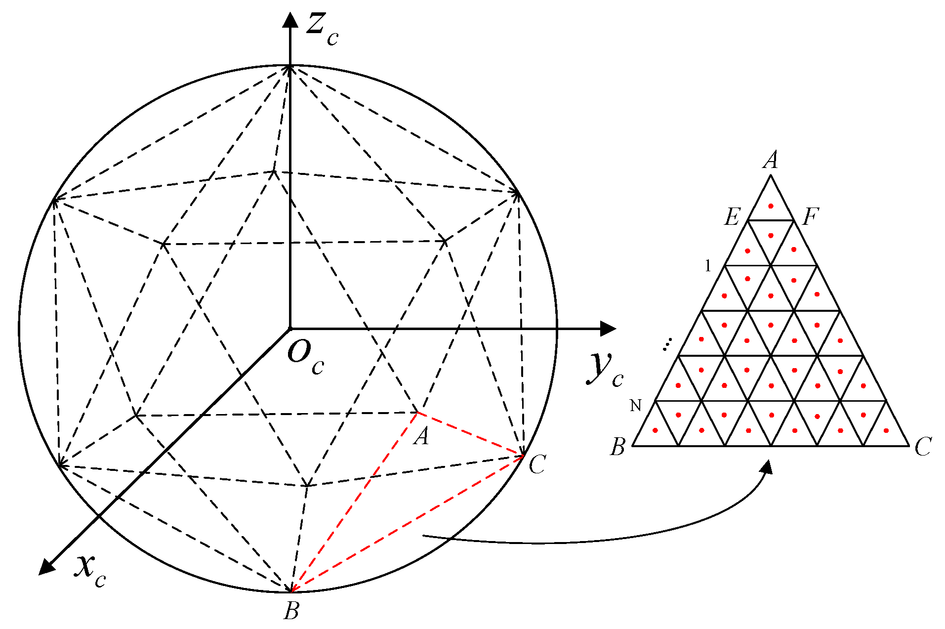
Generally, in a star catalog, the right ascension is in the range of , and the declination is in the range of . During the work of the star sensor, its field of view limits it to capturing only a portion of the sky, meaning only a subset of stars in the star catalog is included in the field of view of the star sensor. However, the majority of algorithms require repeated retrieval of stars from the entire star catalog during the star identification process. This frequent retrieval increases the time taken for feature matching, which easily leads to redundant and false matching and significantly affects the identification speed and rate. Therefore, we propose a method for uniform partitioning of the star catalog which approximates the entire celestial region as a celestial sphere, evenly divides the celestial sphere into several regions, and maps them to the stars in the star catalog.
As illustrated in
Figure 2,
depicts a celestial coordinate system, and connections between the center of the celestial sphere
and the vertices of an arbitrary face in a regular icosahedron form a pyramid. The pyramid intersects with the celestial sphere, uniformly dividing it into 20 regions, each of which is numbered
. Each of these 20 regions is uniformly further subdivided into
zones, resulting in a total of
zones across the entire celestial sphere. The theoretical range for
is
, but the appropriate value should be chosen based on the field of view of the star sensor in practical applications. Once parameter
is determined, the stars in the star catalog are mapped to the corresponding celestial sphere zones to complete the star catalog partitioning.
Taking the regular triangle
in
Figure 2 as an example, let the spatial coordinates of vertex
be
, vertex
be
, and vertex
be
. Then, the spatial coordinate of any point within the triangle
can be expressed as follows:
where
and
are the weight values.
Defining the spatial coordinate of a star
on the celestial sphere as
, the ray equation from the center of the celestial sphere
to the star
can be represented as follows:
where
is a weight value.
If the star
belongs to the celestial sphere zone corresponding to triangle
, then the ray
intersects with triangle
, meaning that there is a common solution between Formulas (2) and (3), which implies the existence of a set of weight values
,
,
that satisfy the following:
Letting
,
and
, Formula (4) is updated to the following:
Solving Equation (5) results in the following:
If the solution of Equation (6) satisfies
and
, the star
belongs to the celestial sphere zone corresponding to triangle
; conversely, the star X does not belong to the zone.
Figure 3 visually demonstrates the scenario in which the star belongs to the celestial sphere zone. The ray from the center of the celestial sphere to the star intersects with the equilateral triangle in the regular icosahedron corresponding to the celestial sphere zone.
Following the described method, the star catalog can be partitioned. Firstly, a zone from the
celestial sphere zones is selected and the vertex coordinates of its corresponding equilateral triangle are obtained. The star catalog is traversed and the zone number is assigned to the star that belongs to the celestial sphere zone. The above process is repeated until each star in the star catalog owns a unique zone number.
Figure 4 visually demonstrates the result of the star catalog partitioning when
. As shown in the figure, the star catalog is uniformly divided into 20 regions, labeled
.
3. Star Identification
Based on the partitioned star catalog, the method for the construction of the navigation feature library is explained in
Section 3.1, and then a voting-based star identification algorithm is proposed in
Section 3.2.
3.1. Construction of Navigation Feature Library
The navigation feature library is a database that characterizes the information of the stars in a star catalog and their positional relationships, serving as the foundation for star identification. The construction quality of the navigation feature library directly impacts the performance of star identification algorithms. Subgraph isomorphism methods typically use the angular distances between two stars as a feature to build the navigation feature library. However, due to the vast number of stars in the star catalog, the navigation feature library generated from angular distances between any two stars will be extremely large. In the process of star identification, the high number of feature matches leads to slow matching speed and a high probability of redundant and false matching, significantly affecting the identification speed and rate. Therefore, we propose a method for constructing a navigation feature library based on the partitioned star catalog.
In
Figure 5, the red circle represents the field of view (FOV) of the star sensor. By selecting an appropriate parameter
, the celestial sphere zone could include the FOV of the star sensor. The stars within the FOV of the star sensor generally belong to several celestial sphere zones rather than one zone, but it is evident from
Figure 5 that the thirteen partitions around partition 0 can definitively contain all stars within the FOV. Therefore, by using thirteen partitions as a basic unit to construct the navigation feature library, the all-sky star identification can be simplified to star identification within the local celestial sphere, which will significantly simplify the navigation feature library and narrow the retrieval region during star identification, thereby markedly enhancing identification speed while effectively reducing the probability of redundant and false matching. The basic unit is constructed using the angular distance between two stars.
Firstly, two stars
and
are randomly selected from thirteen partitions. Then, the reference vectors of two stars are defined as follows:
where
and
are the right ascension and declination of stars
and
.
The angular distance between stars
and
is given by the following:
where the symbol ‘
’ represents the dot product of the vectors, and ‘| |’ is the norm of the vector.
Due to the limitation imposed by the FOV of star sensor, any angular distance within the basic unit that exceeds the FOV is considered as invalid information. Therefore, the constructed basic unit can be optimized based on Formula (9) by filtering out angular distances greater than the FOV.
where
represents the FOV, and
refers to the basic unit
.
Since the arrangement of angular distances within the basic unit is somewhat disorganized, it makes it difficult to perform fast retrieval during star identification. To enhance the retrieval speed of angular distances in the basic unit, we sort the angular distances in ascending order and divide the basic unit into
blocks. Then, an index function as defined in Formula (10) is established to quickly locate the block of the angular distance.
where
denotes rounding to the nearest integer, and
and
represent the minimum and maximum values of the angular distances in the basic unit, respectively. The result
refers to the block number where the angular distance
is located, and its range satisfies
.
3.2. Star Identification Algorithm Based on Voting Decision
The core of star identification uses an algorithm to match the features of stars between the star image and the navigation feature library, thus obtaining information about the stars. The navigation feature library uses the angular distance between stars as a feature; therefore, obtaining the angular distance between stars in the star image is necessary.
The imaging model of the star sensor can be approximated as a pinhole model. The starlight from infinity is treated as parallel light, which is projected onto the surface of the image sensor through the optical system, and then the stars on the image sensor are created.
Figure 6 shows the imaging model of the star sensor.
As shown in
Figure 6,
depicts a coordinate system of a star sensor, and
and
are the projections of stars on the surface of the image sensor, with their centroid coordinates being
and
, respectively. The observation vectors for the stars
and
are
and
, which are calculated as follows:
where
represents the focal length of the star sensor.
Similar to Formula (8), the angular distance between stars
and
is given by the following:
To effectively match the features of stars between the star image and the navigation feature library, a star identification algorithm based on a voting decision is proposed. During the optical system manufacturing of the star sensor, distortion is inevitable and the closer it is to the edge of the FOV, the greater the distortion will be. Therefore, selecting the stars closer to the center of the FOV is advisable during star identification, which could reduce the impact of distortion. As shown in the schematic star image in
Figure 7, we choose those stars within the 3/4 FOV for star identification, and the stars near the edge of the FOV are discarded.
Assuming there are
stars within the 3/4 FOV of the star sensor, the
angular distances between these stars form the set
. In the basic unit
of the navigation feature library, all the angular distances in the set
are sequentially searched. Based on the search results, voting is conducted for
by the following method:
where
represents the voting score of the basic unit
,
represents the angular distance between stars
and
in
,
represents the angular distance between stars
and
in the basic unit
, and
is the error threshold.
As shown in Formula (13), if two stars and in the basic unit could obtain the angular distance and , equal within the error threshold , then the stars and match the stars and . In this case, the voting score of the basic unit increases; otherwise, remains unchanged.
Since the number of angular distances in set is , the theoretical maximum voting score for the basic unit is . However, considering the potential presence of false stars in the FOV, when the voting score of basic unit satisfies , which indicates that at least two sets of feature triangles in the star image belong to the basic unit , the decision can be made that the basic unit matches the angular distance set and is the subset of . Based on this, the basic unit is continually used to identify other stars in the star image. On the contrary, if all angular distances in the set have been traversed and the voting score of basic unit satisfies , which indicates that no feature triangle in the star image belongs to the basic unit , the decision can be made that the basic unit does not match the angular distance set , and it is necessary to select another basic unit and repeat the process above.
5. Nighttime Stargazing Experiment
In this section, the performance of the proposed algorithm is verified through a nighttime stargazing experiment. To reduce the interference of stray light on the experiment, the observation site is selected at the Xinglong Station of the National Astronomical Observatory, Chinese Academy of Sciences, located in Xinglong County, Chengde City, Hebei Province. The geographical coordinates are 117°34′30″ E longitude, 40°23′36″ N latitude, and the site is located at an altitude of 960 m. The experiment is conducted on a clear night, and the equipment mainly includes a large-aperture telescope and a star sensor. The key parameters of the star sensor are listed in
Table 1.
As shown in
Figure 12, the star sensor is fixed on the telescope, ensuring that the coaxial and star sensor are unobstructed. The telescope provides directional guidance to the star sensor based on star catalog information from the control software of the telescope.
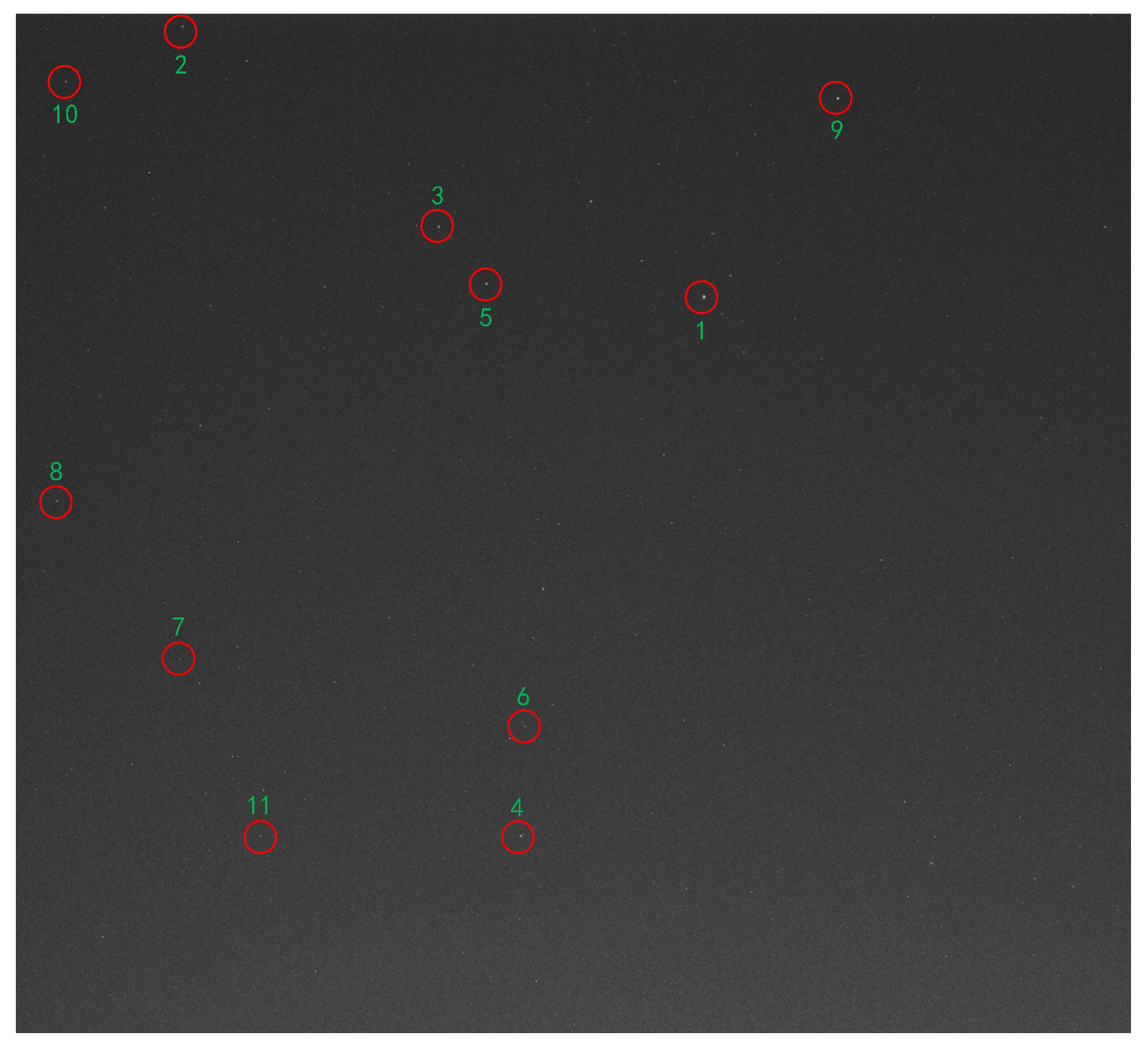
During the experiment, a celestial region is firstly selected in the star catalog from the control software, and then the telescope and star sensor are guided to point at the selected region. As shown in
Figure 13, the star sensor captures a star image and the stars are identified using the star identification algorithm.
The information of the identified stars is explained in
Table 2, and includes centroids, average gray value, right ascension, declination, and magnitude.
Based on the right ascension and declination information listed in
Table 2, the corresponding celestial region of the star image is captured and shown in
Figure 14.
It is pretty obvious that the relative positions of the stars in
Figure 13 and
Figure 14 are virtually identical, and the right ascension, declination, and magnitude of the stars shown in
Figure 14 are largely consistent with the information in
Table 2, which confirms the validity of the proposed star identification algorithm.
In addition, the star information in
Table 2 has been sorted in the sequence of ascending magnitude. Based on this, the histogram regarding the gray value and magnitude of the stars is generated and shown in
Figure 15.
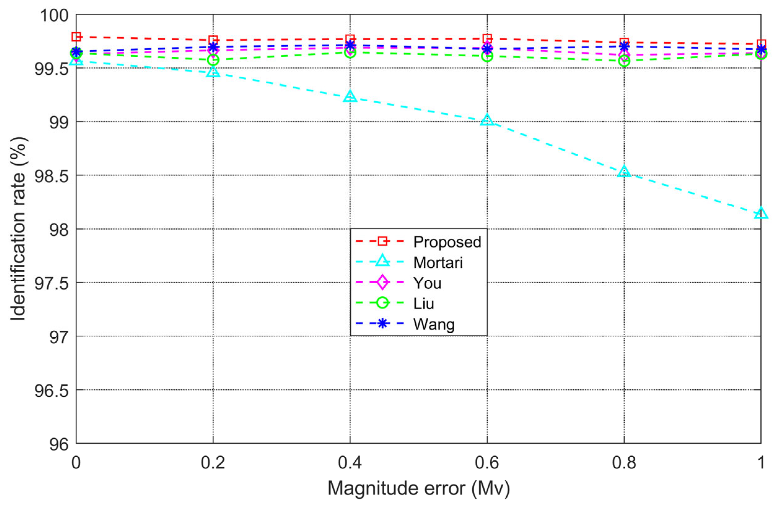
Generally, higher magnitude corresponds to lower brightness; however, as shown in
Figure 15, the gray values of stars do not consistently decrease as the magnitude increases. Specifically, star 9, with a magnitude of only 4.36, has a significantly higher gray value than star 2, which has a magnitude of 3.19. This indicates that a magnitude error is indeed present in the star image when the star sensor works in practice. Nevertheless, the proposed algorithm successfully identifies the star image, even with significant brightness interference, further demonstrating the robustness of the proposed algorithm against the magnitude error. The robustness is attributed to the fact that the brightness of star is not used as a feature during the process of star identification, making the algorithm less susceptible to the effect of magnitude errors. To thoroughly validate the identification performance of the proposed algorithm, the rotation of the telescope is controlled and the star sensor is guided to capture 5000 frames of star images corresponding to different celestial regions. Different star identification algorithms are applied to identify the stars in the star images, and the average identification rate and average identification time for each algorithm are recorded and listed in
Table 3.
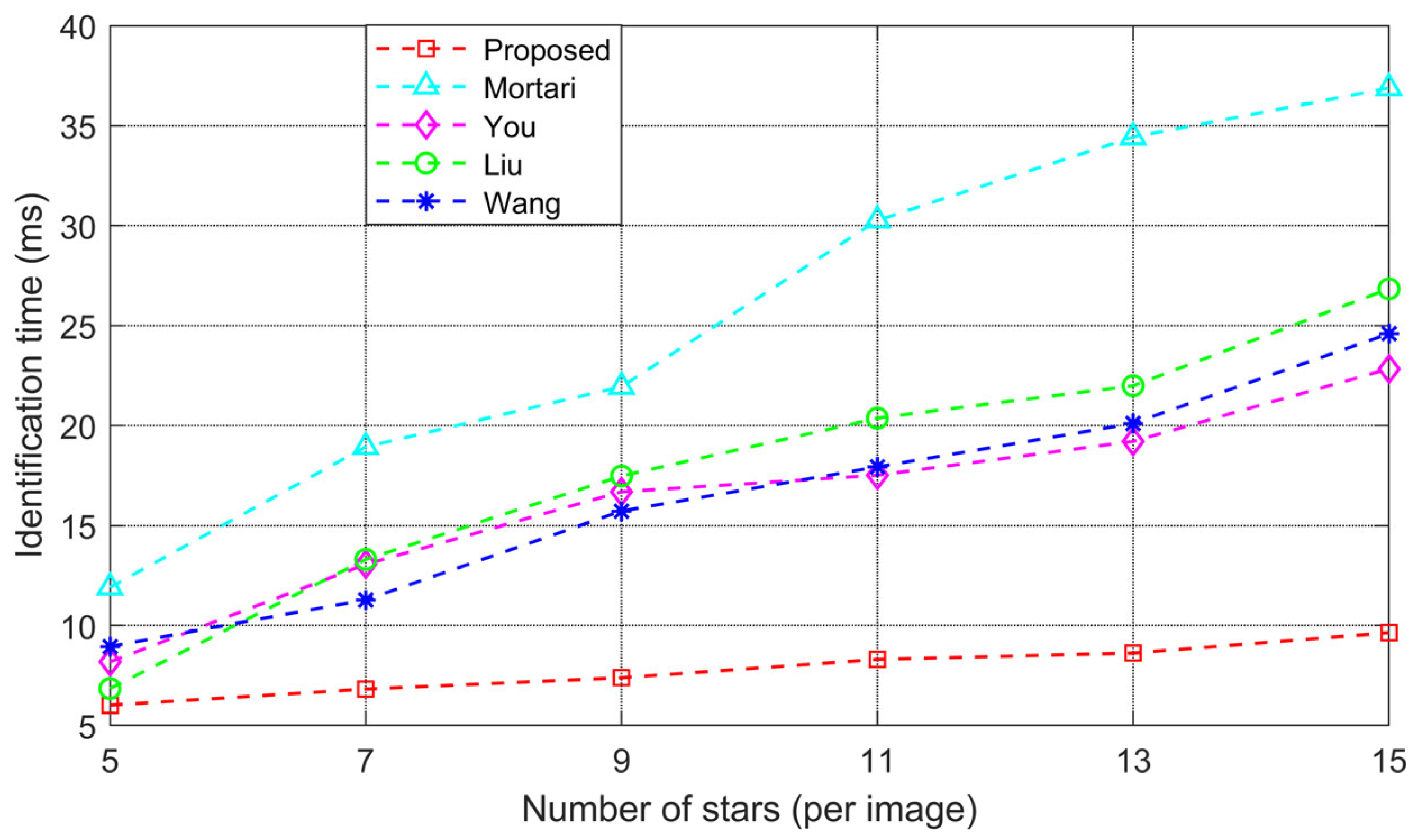
The results in
Table 3 demonstrate that, under the same experimental conditions, the proposed algorithm achieves an average identification rate of 99.760% and an average identification time of 8.861 milliseconds. Both the identification rate and time are significantly better than those of the other algorithms, further confirming the effectiveness of the proposed star identification algorithm in the application of a star sensor.


