Improvement of Dung Beetle Optimization Algorithm Application to Robot Path Planning

Abstract

We propose the adaptive t-distribution spiral search Dung Beetle Optimization (TSDBO) Algorithm to address the limitations of the vanilla Dung Beetle Optimization Algorithm (DBO), such as vulnerability to local optima, weak convergence speed, and poor convergence accuracy. Specifically, we introduced an improved Tent chaotic mapping-based population initialization method to enhance the distribution quality of the initial population in the search space. Additionally, we employed a dynamic spiral search strategy during the reproduction phase and an adaptive t-distribution perturbation strategy during the foraging phase to enhance global search efficiency and the capability of escaping local optima. Experimental results demonstrate that TSDBO exhibits significant improvements in all aspects compared to other modified algorithms across 12 benchmark tests. Furthermore, we validated the practicality and reliability of TSDBO in robotic path planning applications, where it shortened the shortest path by 5.5–7.2% on a 10 × 10 grid and by 11.9–14.6% on a 20 × 20 grid.

1. Introduction

With the rapid development of various industries, many optimization problems arise in real life. Real-world optimization problems are usually very complex and computationally difficult [1,2]. To address these challenges effectively, metaheuristic algorithms are applied.

Significant progress has been made in metaheuristic algorithms in recent years. These algorithms can be broadly categorized into two types: population-based algorithms and evolution-based algorithms [3]. Evolution-based algorithms are inspired by biological evolution principles. Genetic Algorithm (GA) [4] is a typical example of this theory. Similarly, the widely studied Differential Evolution (DE) [5] simulates natural processes like survival of the fittest and biological evolution. Population-based algorithms provide solutions by distributing information about all participants in the optimization. One of the better such algorithms in recent years is the Sparrow Search Algorithm (SSA) proposed by Xue et al., which simulates the behavior of sparrows while foraging and avoiding predators [6]. By simulating the foraging and storage behaviors of starlings in summer and fall as well as the memory-based food-seeking behaviors in winter and spring, Mohamed et al. proposed the Nutcracker Optimization Algorithm (NOA) [7]. Wang et al. proposed the Black-winged Kite Algorithm (BKA) in 2024 [8], inspired by black-winged kite migration and foraging behaviors. And other similar algorithms include Wild Horse Optimizer (WHO) [9], Golden Jackal Optimization (GJO) [10], Sea-horse Optimizer (SHO) [11], the Greater Cane Rat Algorithm (GCRA) [12], and Red-billed Blue Magpie Optimizer (RBMO) [13].

Based on the better performance of these algorithms, many scholars have improved the basic algorithms and proposed some improved algorithms with better results. Li et al. integrated the sine–cosine algorithm and the Cauchy variational strategy into SSA to obtain SCSSA [14]. Inspired by the techniques of opposition-based learning (OBL) and randomized opposition-based learning (ROBL), Sarada proposed a fast randomized opposition-based learning Golden Jaguar optimization algorithm (FROBL-GJO) [15] to improve the GJO algorithm’s optimization accuracy and convergence speed. Mohamed et al. combined the sine–cosine algorithm with the hippocampus optimization algorithm to obtain the Sea-horse Optimizer Sine Cosine Algorithm (SHOSCA) [16].

The improvement of metaheuristic algorithms is not only important in the theoretical setting, but also crucial in practical applications. Efficient path planning can help robots accomplish tasks better and reduce the waste of resources. Shen et al. proposed the Elite Preserving Differential Evolutionary Gray Wolf Optimizer (EPDE-GWO) [17] in order to optimize the Vertical Farming System Multi-Robot Trajectory Planning Model (VFSMRTP). In order to optimize the path planning of warehouse logistics robots and improve the shortest route and smoothness of the path, You et al. proposed the multi-strategy Integrated Whale Algorithm (IWOA) [18]. Łukasz applied the Gray Wolf Optimizer to the Constrained Optimization Problem for a line-start PM Motor [19]. Li et al. proposed a multi-strategy improved Harris Hawk optimization algorithm (MIHHO) [20]. This algorithm aims to overcome challenges in indoor mobile robot path planning, such as local shortest paths, slow search speed, and low path accuracy. The path planning problem must consider path length, computation time, and path feasibility [21]. Traditional metaheuristic algorithms do not take these aspects into account at the same time, and it is difficult to find a balanced solution. So, this study is challenging.

In 2022, Xue et al. proposed the Dung Beetle Optimization Algorithm (DBO) [22]. Like many other metaheuristic algorithms, DBO faces challenges such as slow convergence speed, low convergence accuracy, and a tendency to get stuck in local optima. These problems were addressed by developing an improved version of DBO, known as TSDBO, which was successfully applied to the two-dimensional robot path planning problem. Although this paper focuses on the 2D robot path planning problem, through comprehensive benchmark function testing and solving real-world application problems, the adaptability and performance of TSDBO show its potential applicability in other optimization problems. The following is a summary of this paper’s primary innovations and contributions:

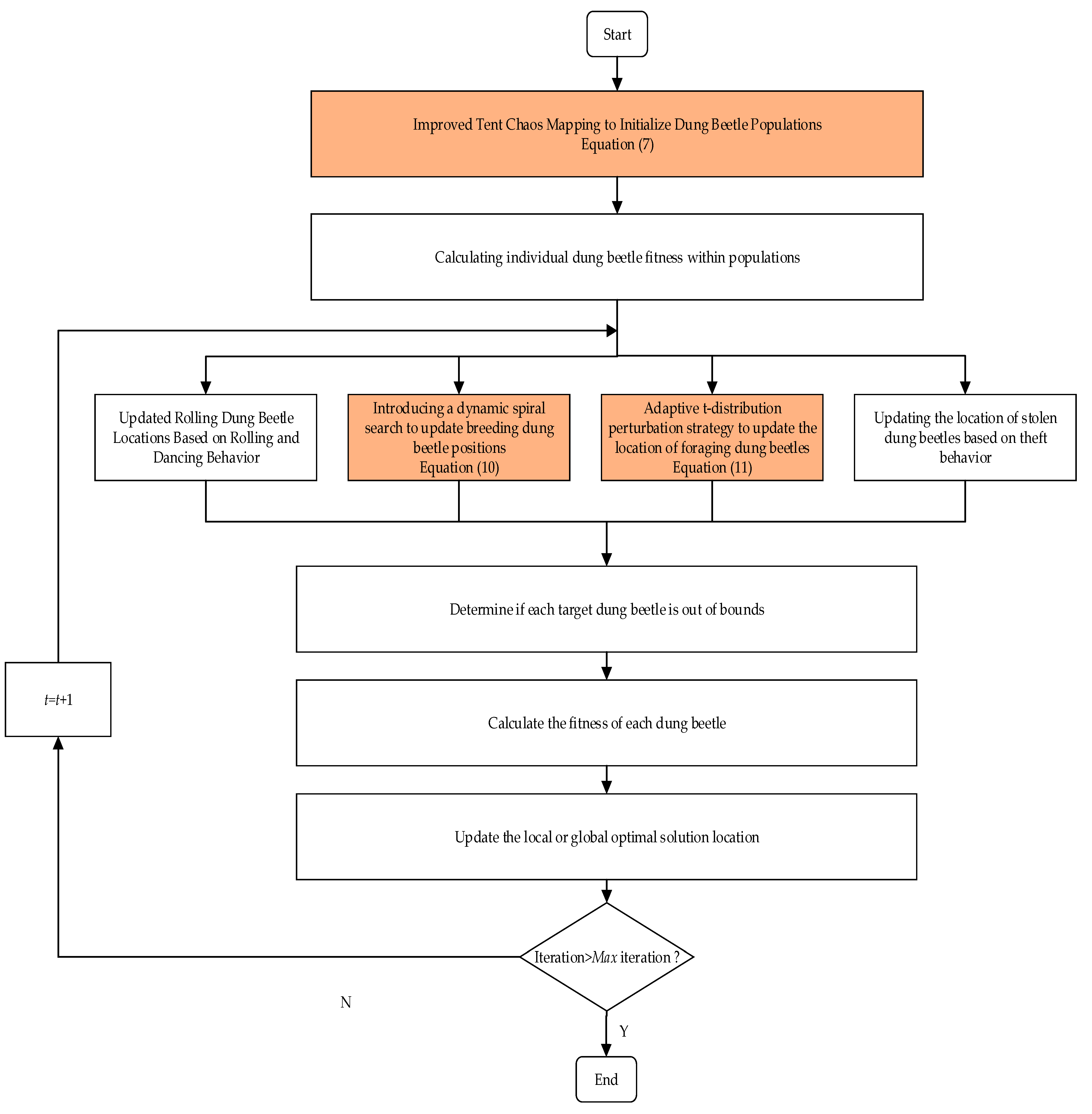
• The TSDBO algorithm incorporates an improved Tent chaotic mapping in the initialization phase to enhance the distribution of dung beetles in the solution space. A dynamic spiral search strategy is introduced during the reproduction phase to boost global search capability and efficiency. In the foraging phase, an adaptive t-distribution perturbation strategy helps the small dung beetles escape local optima and accelerates the convergence rate.
• To assess TSDBO, twelve benchmark functions were chosen from the CEC2005 set. TSDBO shows better all aspects than other algorithms in the evaluation of twelve benchmark functions from the CEC2005 set.
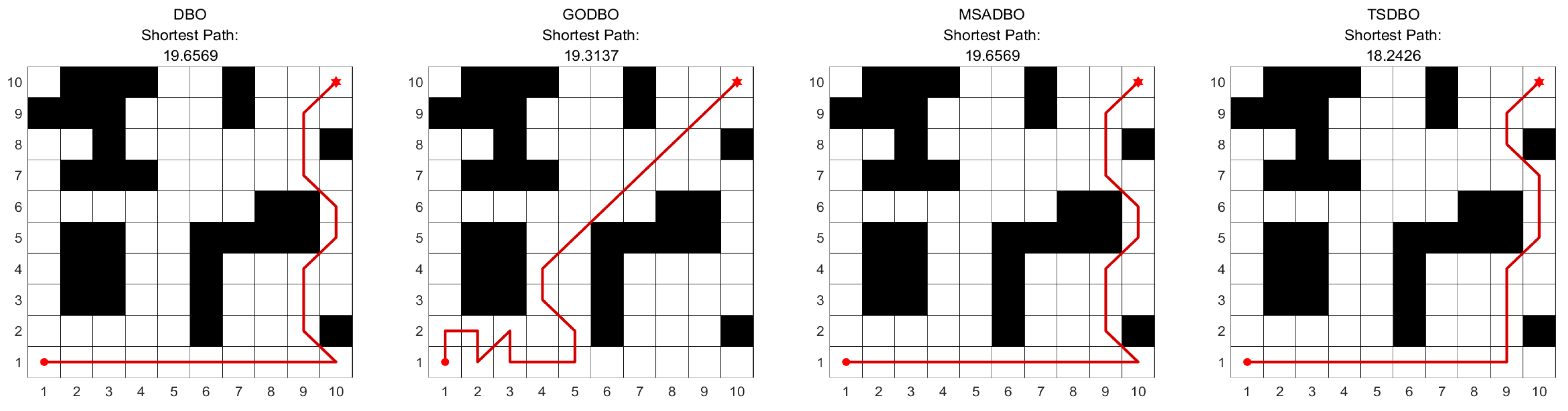
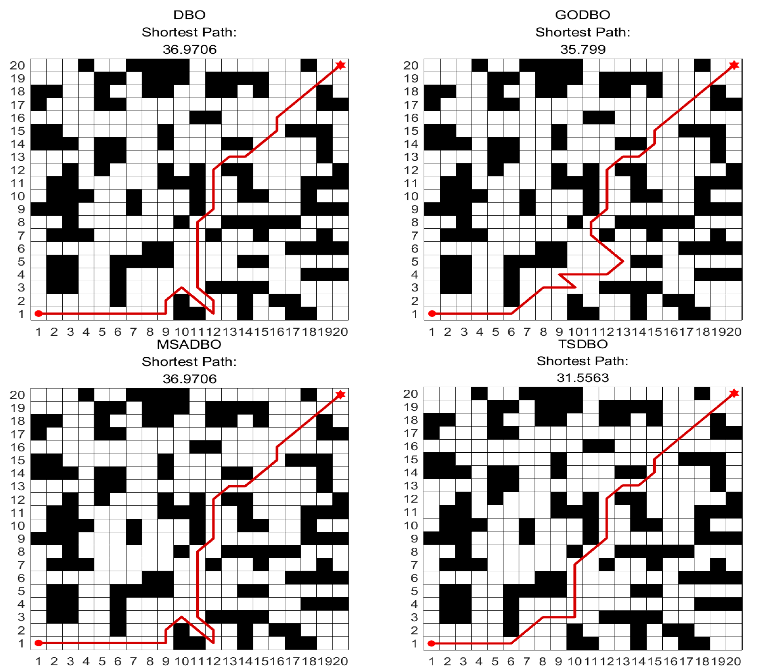
• TSDBO demonstrated its efficacy in generating shorter paths in comparison to alternative algorithms when applied to the 2D robot path planning challenge.

The remainder of this paper is organized as follows: The approach and related works are introduced in Section 2. In Section 3, the suggested TSDBO algorithm is described in full. The experimental data and findings are presented and discussed in Section 4. Conclusions and future work are covered in Section 5 at the end.

2. Related Works and Method

2.1. Related Works

Scholars have used the DBO algorithm in practical problems. In a previous study [23], the DBO algorithm was employed for photovoltaic array fault diagnosis. It was integrated with Long Short-Term Memory (LSTM) networks to construct an effective fault diagnosis model. The authors of [24] proposed an enhanced multi-strategy dung beetle algorithm, and the improved algorithm was used for trajectory planning in a 3D environment; the results showed that the paths can be planned to avoid hazardous sources in a safer and more effective way. The authors of [25] proposed the MIDBO algorithm; experiments demonstrated that the MIDBO method outperforms the alternative approach.

In order to use robots in real life, the robot path planning problem is fundamental. The essence of this is to plan a feasible path for the robot that connects the starting point to the end point and satisfies the actual constraints. Traditional path planning methods mainly include the Dijkstra algorithm [26], A* algorithm [27], artificial potential field method [28], RRT [29], etc. However, these traditional methods face limitations in dynamic or complex environments. For example, they struggle with generating smooth paths and meeting real-time response requirements. Additionally, their performance is constrained in high-dimensional spaces or nonlinear optimization problems, making them less suitable for path planning in intricate environments [30]. The emergence of metaheuristic algorithms provided a new solution to this problem. In recent years, metaheuristic algorithms have stood out for their better robustness, global search capability, and adaptability [31].

Traditional metaheuristic algorithms for path planning include particle swarm optimization (PSO) [32], ant colony optimization (ACO) [33], the firefly algorithm (FA) [34], etc. PSO has a faster convergence speed, but while working with complicated surroundings and multi-peak situations, the performance is unsatisfactory. ACO has stronger global search capability [35], but has high computational complexity and a slower convergence speed [36,37]. FA has powerful diversified search capability, but is not adaptable enough in dealing with complex environments. Although these algorithms are capable of global search and path optimization, they are often limited in their ability to efficiently handle complex problems, plan paths effectively, and minimize computational overhead. TSDBO improved the algorithm’s flexibility in intricate settings and its ability to satisfy path planning requirements.

The DBO algorithm demonstrates strong optimization capabilities and fast convergence, inspired by the dung beetle’s natural foraging behavior. However, it faces several challenges, such as an uneven distribution of the initial population, an imbalance between local exploitation and global exploration, and a tendency to get trapped in local optima. Despite these limitations, the biologically inspired search process of DBO has garnered significant attention in the field of robot path planning. However, poor convergence, limited adaptation to dynamic impediments, and the inability to update pathways in real time are some of the problems that traditional DBO faces [38]. Nevertheless, it is a strong contender for path planning applications due to its capacity for global search and path optimization.

2.2. Method

Dung beetles update their positions in parallel in different ways and finally select the optimal solution. The proportions of various dung beetles in the population are 20%, 20%, 25%, and 35% [22].

(1)

Rolling behavior

Celestial navigation is used by dung beetles during the rolling process to keep the ball of dung rolling in a straight trajectory. The environment influences the dung beetle’s rolling path, and the dung beetle’s position is impacted by changes in the surrounding environment. The rolling behavior is represented by Equations (1) and (2).

$$\left\{\begin{array}{c}{x}_i\left(t+1\right)=x_i\left(t\right)+\alpha \times k\times x_i\left(t-1\right)+b\times \Delta x\\ \Delta x=\left|\left.x_i\left(t\right)-X^w\right|\right.\end{array}\right.$$

(1)

$$x_i\left(t+1\right)=x_i\left(t\right)+\tan \left(\theta \right)\left|\left.x_i\left(t\right)-x_i\left(t-1\right)\right|\right.$$

(2)

In Equation (1), $t$ is the current iteration number, $x_i(t)$ represents the position information of the $i$th dung beetle at the $t$th iteration, $k$ is a constant between (0,0.2], we choose $k$ to be 0.1, $b$ is a constant between (0,1), and we choose it to be 0.3, and $\alpha$ is a natural coefficient of −1 or 1, which represents the natural factor. When $\alpha$ is −1, it means that the dung beetle encounters obstacles in the process of moving forward, and the direction deviates. When $\alpha$ is 1, it means that the dung beetle has no obstacles and the direction does not deviate. $X^W$ is the global worst position, and $\Delta x$ is the environmental variation.

In Equation (2), $x_i\left(t\right)-x_i\left(t-1\right)$ is the difference between the position of the $i$th dung beetle at the $t$th iteration and the position at the $t-1$st iteration. It can be seen that the position update of the rolling dung beetle is closely related to the current and historical information. If the angle is 0, π/2, π, then the position of the dung beetle is not updated.

(2)

Reproductive behavior

Each female dung beetle lays only one egg at a time after deciding on a good spawning location by rolling their dung balls to a safe location and then hiding. The number of iterations dynamically modifies the spawning area, and the egg ball’s position correspondingly changes, which is expressed by Equation (3).

$$B_i\left(t+1\right)=X^{\ast }+b_1\times \left(B_i\left(t\right)-L{b}^{\ast }\right)+b_2\times \left(B_i\left(t\right)-U{b}^{\ast }\right)$$

(3)

In Equation (3), $X^{\ast }$ is the current local optimal position, $L{b}^{\ast }$ and $U{b}^{\ast }$ are the lower and upper limits of the spawning area, $B_i\left(t\right)$ denotes the position of the $i$th sphere at the $t$th iteration, $b_1$ and $b_2$ are independent random vectors of $1\times D$, and $D$ is the dimension of the optimization problem.

(3)

Foraging behavior

To lead the small dung beetle to forage once the larvae hatch, the ideal foraging area must be determined. Equation (4) expresses the process.

$$x_i\left(t+1\right)=x_i\left(t\right)+C_1\times \left(x_i\left(t\right)-L{b}^b\right)+C_2\times \left(x_i\left(t\right)-U{b}^b\right)$$

(4)

In Equation (4), $L{b}^b$ and $U{b}^b$ are the lower and upper bounds of the optimal foraging area. $C_1$ is a random number that follows a normal distribution, and $C_2$ is a (0,1) random number.

(4)

Stealing behavior

In dung beetle populations, taking food made by other dung beetles is a common competitive action. Equation (5) represents the positional update of the stealing dung insects.

$$x_i\left(t+1\right)=X^b+S\times g\times \left(\left|\left.x_i\left(t\right)-X^{\ast }\right|\right.+\left|\left.x_i\left(t\right)-X^b\right|\right.\right)$$

(5)

In Equation (5), $X^b$ is the optimal food source, $S$ is a constant, and $g$ is a $1\times D$ random vector obeying a normal distribution.

3. The Proposed Algorithm

To address the shortcomings of the Dung Beetle Optimization (DBO) Algorithm, including its slow speed, poor optimization accuracy, and tendency to get trapped in local minima, three optimization strategies are proposed to enhance the basic DBO. These strategies aim to improve the algorithm’s overall performance and efficiency. First, to improve the dispersion of the dung beetle population and facilitate subsequent optimization steps, the population is initialized using an upgraded Tent chaos mapping technique. This adjustment enhances the initial population’s diversity, setting a strong foundation for the optimization process. Second, a dynamic spiral search method is introduced to enhance the algorithm’s global optimization capability and search efficiency. This strategy specifically targets the breeding phase of the algorithm, allowing it to explore the search space more effectively and avoid premature convergence. Finally, during the foraging phase of the smaller dung beetles, an adaptive t-distribution perturbation strategy is applied. This technique accelerates the algorithm’s convergence speed and helps the algorithm escape local minima by enabling more effective local search exploration. The following sections provide a detailed description of each of these enhancement strategies.

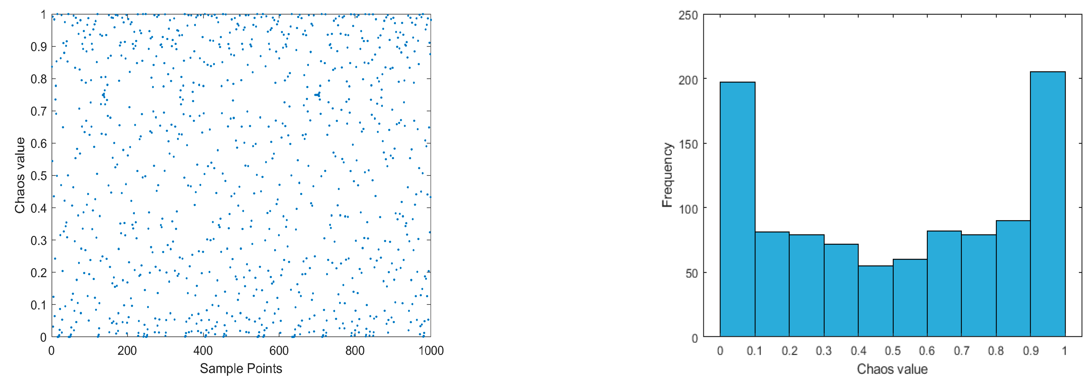
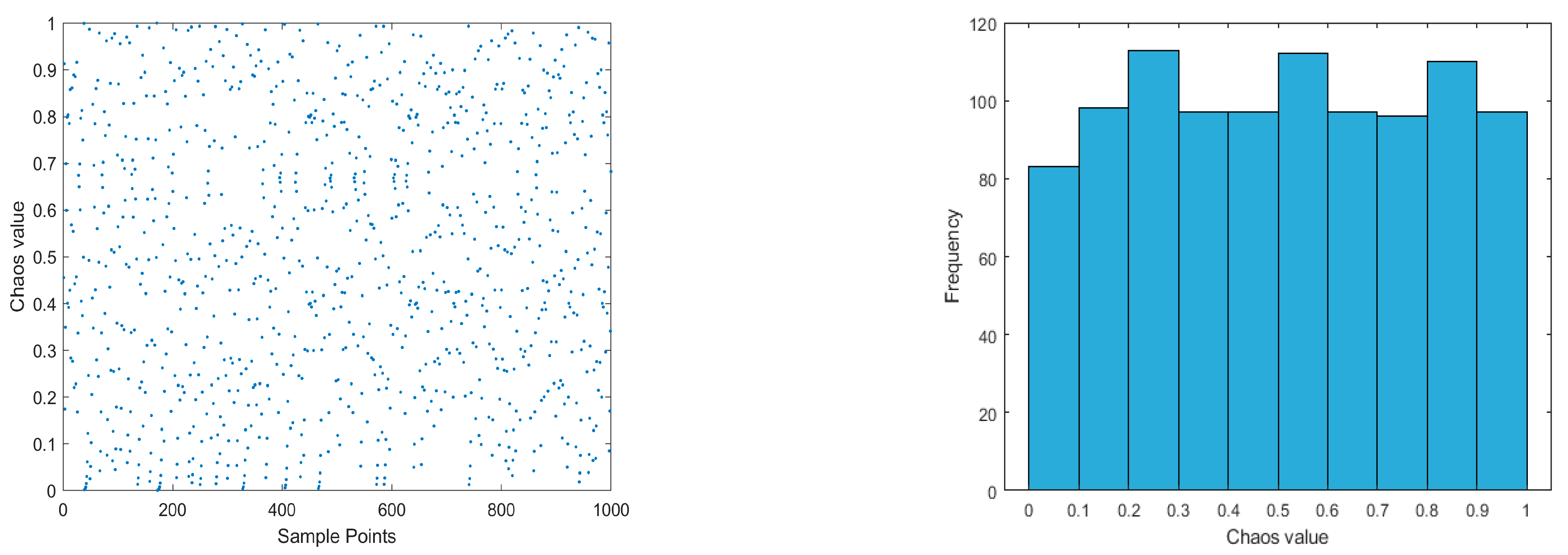
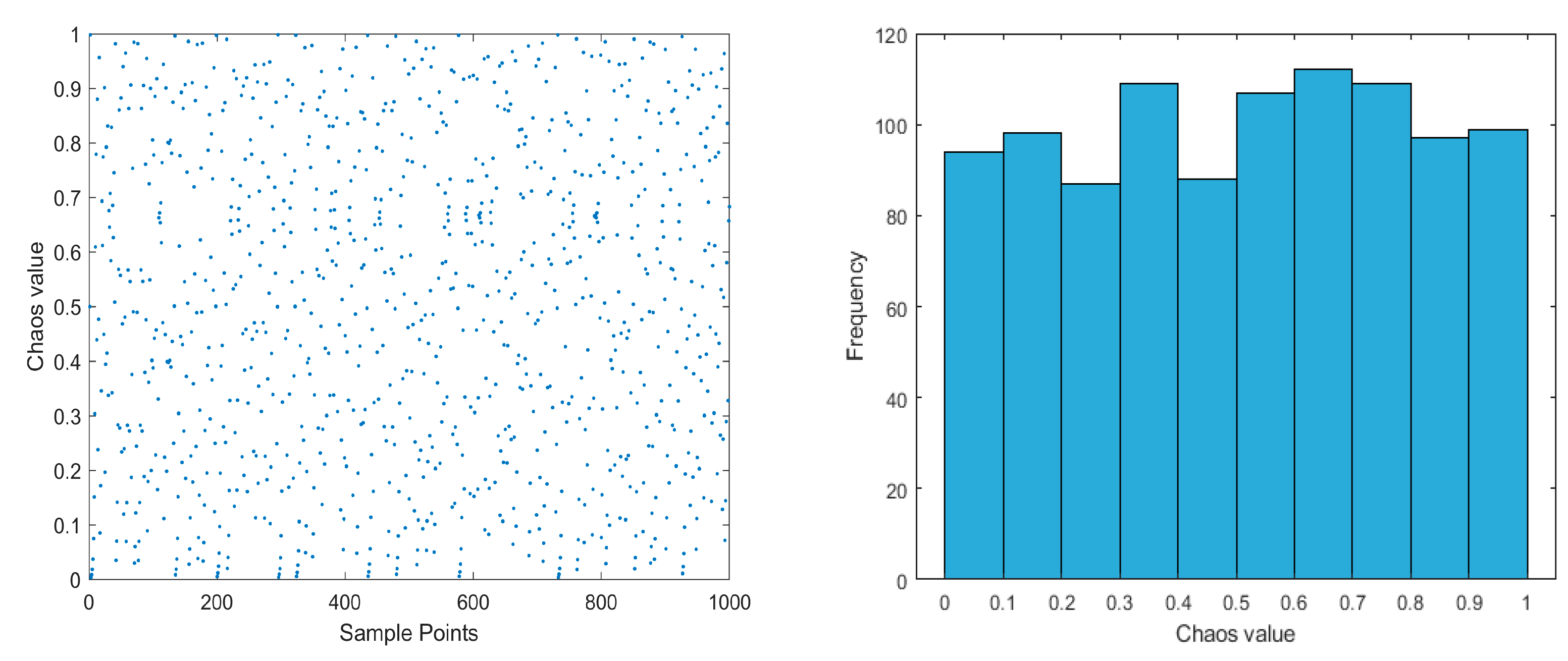
3.1. Improved Tent Chaos Mapping Strategy

Similar to other metaheuristic optimization algorithms, the original Dung Beetle Optimization (DBO) Algorithm initializes the population by randomly assigning individual positions. However, this random initialization often leads to low population diversity and slow convergence, especially when dealing with complex problems. To address this issue and promote a more even distribution of individuals across the solution space, we propose initializing the population using a chaotic mapping technique. This approach enhances the diversity of the initial population, which can improve the overall search efficiency and convergence speed of the algorithm.

Chaotic perturbation functions frequently cited in the literature include the Logistic and Tent mappings. The Logistic mapping is known for its uniform probability distribution in the center of the range, with a significantly higher probability at the boundaries. However, this distribution can be less effective in optimization problems where the global optimum is not near the boundaries of the design space. In contrast, the Tent mapping typically offers better performance compared to the Logistic mapping [39]. The Tent mapping provides a more balanced distribution of values across the entire range, which enhances the algorithm’s ability to explore the solution space more effectively. Figure 1 illustrates the chaotic sequence generated by the Logistic mapping, while Figure 2 shows the chaotic sequence generated by the Tent mapping.

As observed, Logistic chaotic maps have a significantly higher probability of generating values near the boundaries, while Tent chaotic maps offer a more uniform probability distribution across the feasible domain. Consequently, if Logistic chaotic mapping is used to initialize the population, the inhomogeneity of its chaotic sequence can negatively impact the speed and accuracy of the algorithm’s optimization. In this paper, we utilize Tent chaotic mapping to initialize the population instead of random initialization. This approach is favored because the Tent chaotic mapping provides a more evenly distributed population compared to those generated by Logistic chaos mapping or random initialization. The Tent chaotic mapping is mathematically represented by Equation (6).

$$x_{i+1}=\left\{\begin{array}{c}2x_i\hspace{1em}\hspace{1em}\hspace{1em}\hspace{1em}0⩽x⩽{\displaystyle \frac{1}{2}},\hfill \\ 2(1-x_i){\displaystyle \hspace{1em}\hspace{1em}\frac{1}{2}}<x⩽1.\hfill \end{array}\right.$$

(6)

Through the analysis of the Tent chaotic iteration sequence, we identified the presence of unstable cycle regions and small cycles. These cycles can cause the sequence to become trapped, leading to ineffective exploration of the solution space. To mitigate this issue and prevent the sequence from getting stuck in these cycles, we introduced a random variable into the original Tent chaotic mapping. This modification enhances the mapping’s ability to explore the solution space more effectively and avoids the repetitive patterns found in small cycles. This adjustment allows for better population initialization by ensuring greater diversity and improving the algorithm’s performance in complex optimization tasks. The enhanced Tent chaotic mapping is expressed by Equation (7).

$$x_{i+1}=\left\{\begin{array}{c}2x_i+rand\left(0,1\right)\times {\displaystyle \frac{1}{N}\hspace{1em}\hspace{1em}\hspace{1em}\hspace{1em}}0⩽x⩽{\displaystyle \frac{1}{2}},\hfill \\ 2(1-x_i)+rand\left(0,1\right)\times {\displaystyle \frac{1}{N}}{\displaystyle \hspace{1em}\hspace{1em}\frac{1}{2}}<x⩽1.\hfill \end{array}\right.$$

(7)

In Equation (7), $N$ is how many particles there are in the sequence. In addition to maintaining the Tent chaotic mapping’s regularity, ergodicity, and randomness, the $rand\left(0,1\right)/N$ successfully keeps the algorithm from slipping into tiny, unstable cycles while iterating. Figure 3 displays the impact of the enhanced Tent chaotic sequence.

As shown in Figure 3, the uniformity of the improved Tent chaotic mapping has been enhanced compared to the original version. This improvement in uniformity ensures a more even distribution of the initial population across the solution space. Therefore, in this study, we replace the previous population initialization method in the DBO with the enhanced Tent chaotic mapping. This change significantly improves the algorithm’s optimization accuracy by enhancing the quality of the initial population’s distribution in the search space, thereby facilitating a more efficient and effective exploration of the solution space.

3.2. Dynamic Spiral Search Strategy

If we track the chicks’ present reproductive process in the spawning location, the DBO algorithm can quickly lead to population convergence. Nevertheless, this can also lead to a reduction in the number of effective individuals within the population, which raises the possibility that the algorithm will become stuck in local optima. In order to optimize Equation (3) for the DBO reproduction phase, in Equation (3), we include the spiral search technique for prey collection by individual whales in the Whale Optimization Algorithm [40]. It can boost individual diversity in addition to guaranteeing the algorithm’s speed of convergence. Equation (8) represents the roundup phase of whale prey.

$$\left\{\begin{array}{c}X\left(t+1\right)=D\prime \times e^{cl}\times \cos \left(2\pi l\right)+X^{\ast }\left(t\right)\\ D\prime =\left|\left.X^{\ast }\left(t\right)-X\left(t\right)\right|\right.\end{array}\right.$$

(8)

However, the defining parameter $c$ readily influences the technique. The algorithm will converge slowly with a small $c$ and decay too quickly with a big $c$, resulting in a local optimum. The dynamic spiral search shape’s parameter $r$, which is represented in Equation (9), is introduced in order to address this issue.

$$r=e^{cg\cos \left({\displaystyle \frac{\pi t}{Max\_iteration}}\right)}$$

(9)

The reproduction phase of the DBO is improved using a dynamic spiral search strategy and the updated DBO is formulated by Equation (10).

$$B_i\left(t+1\right)=X^{\ast }+e^{rl}\times \cos \left(2\pi l\right)\times b_1\times \left(B_i\left(t\right)-L{b}^{\ast }\right)+e^{rl}\times \cos \left(2\pi l\right)\times b_2\times \left(B_i\left(t\right)-U{b}^{\ast }\right)$$

(10)

The algorithm’s global optimal search performance was enhanced by the introduction of the dynamic spiral search strategy, which increases search efficiency and modifies the parameter $r$. According to the spiral properties, the algorithm’s optimization accuracy is also somewhat increased at the same time.

3.3. Adaptive T-Distribution Perturbation Strategy

In the later stages of the basic DBO, individual dung beetles tend to converge quickly, assembling around the current optimal position. However, if this optimal position is not the global optimum, the effectiveness of searching around this area is significantly reduced. This results in wasted search efforts and may cause the algorithm to miss the global optimal solution. The global ideal position plays a crucial role in determining how effectively the smaller dung beetles forage in the DBO algorithm. To address this, the foraging behavior in this study is modeled using a t-distribution perturbation factor, which is dynamically adjusted based on the degrees of freedom corresponding to the number of iterations. This approach allows the algorithm to adjust its exploration capabilities and avoid premature convergence to local optima. The mechanism for updating the positions of the dung beetles is provided by Equation (11).

$$X_{new}^j=X_{best}^j+t\times \left(C\_iter\right)\times X_{best}^j$$

(11)

where $X_{new}^j$ is the mutated small dung beetle position, $X_{best}^j$ is the best small dung beetle position, and $t\left(C\_iter\right)$ is mutated.

The adaptive t-distributed variational perturbation component incorporates both Gaussian and Cauchy distribution characteristics. This hybrid approach enhances the DBO algorithm’s ability to accelerate convergence in the early stages of the optimization process, while also facilitating more effective local exploration in the later stages. The Gaussian distribution allows for efficient exploitation of the search space, particularly in the early iterations, whereas the Cauchy distribution helps avoid local optima by promoting broader exploration during later iterations. By combining these two distribution features, the adaptive perturbation strategy improves the algorithm’s overall balance between global exploration and local exploitation, ensuring better optimization performance throughout the entire search process.

3.4. Algorithm Steps and Algorithm Flow

To provide a more intuitive understanding of the TSDBO algorithm’s implementation process, the Algorithm 1 presents the algorithm’s pseudo-code. The Algorithm 1 outlines the key steps involved in the algorithm, allowing readers to better grasp its structure and operation. Additionally, Figure 4 illustrates the flowchart of the proposed algorithm. The flowchart visually represents the sequence of steps, helping to clarify the logical flow and decision-making processes within the TSDBO algorithm.

Algorithm 1 The framework of the TSDBO algorithm

Require: The maximum iterations TMAX, the size of individuals in the population N, obtain an initialized population X of dung beetles using the improved Tent chaos mapping strategy.

Ensure: Optimal position $X^b$ and its fitness value $f_b$

1: while $t\le TMAX$ do

2: for $i=1$ to Number of rolling dung beetles do

3:   $\alpha =rand(1)$

4:   if $\alpha <0.9$ then

5:    Update rolling dung beetle location by Equation (1).

6:   else

7:    Rolling the ball in the encounter of obstacles by Equation (2) to update.

8:   end if

9:  end for

10:   The value of the nonlinear convergence factor is calculated by $R=1-t/TMAX$.

11:  for $i=1$ to Number of breeding dung beetles do

12:   Updating of breeding dung beetles by Equation (10).

13:  end for

14:  for $i=1$ to Number of Foraging dung beetles do

15:   Updating of foraging dung beetles by Equation (11).

16:  end for

17:  for $i=1$ to Number of Stealing dung beetles do

18:   Updating of stealing dung beetles by Equation (5).

19:  end for

20: Determine if each target dung beetle is out of bounds.

21: Calculate the fitness of each dung beetle.

22 if the newly generated position is better than before then

23:  Update it.

24: end if

25 $t=t+1$

26: end while

27: return $X^b$ and its fitness value $f_b$

4. Results of the Experiment and Discussion

4.1. Description of Test Functions

Table 1. Twelve benchmark functions in CEC2005.

Function Name	D	S	${\mathit{f}}_{\mathbf{min}}$
$f_1\left(x\right)={\displaystyle {\sum }_{i=1}^n{x}_i^2}$	30	[−100, 100]	0
$f_2\left(x\right)={\displaystyle {\sum }_{i=1}^n\left|\left.x_i\right|\right.+{\displaystyle {\prod }_{i=1}^n\left|\left.x_i\right|\right.}}$	30	[−10, 10]	0
$f_3\left(x\right)={{\displaystyle {\sum }_{i=1}^n\left({\displaystyle {\sum }_{j-1}^i{x}_j}\right)}}^2$	30	[−100, 100]	0
$f_4\left(x\right)={\max }_i\left\{\left|\left.x_i\right|,1\le i\right.\le n\right\}$	30	[−100, 100]	0
$f_5\left(x\right)={\displaystyle {\sum }_{i=1}^{n-1}\left[100{\left(x_{i+1}-x_i^2\right)}^2+{\left(x_i-1\right)}^2\right]}$	30	[−30, 30]	0
$f_6\left(x\right)={\displaystyle {\sum }_{i=1}^n-x_i}\sin \left(\sqrt{\left|\left.x_i\right|\right.}\right)$	30	[−500, 500]	−12,569.5
$f_7\left(x\right)={\displaystyle {\sum }_{i=1}^n\left[x_i^2-10\cos \left(2\pi x_i\right)+10\right]}$	30	[−5.12, 5.12]	0
$f_8\left(x\right)=-20\exp \left(-0.2\sqrt{{\displaystyle \frac{1}{n}}{\displaystyle {\sum }_{i=1}^n{x}_i^2}}\right)-\exp \left({\displaystyle \frac{1}{n}}{\displaystyle {\sum }_{i=1}^n\cos \left(2\pi x_i\right)}\right)+20+e$	30	[−32, 32]	0
$f_9\left(x\right)={\displaystyle \frac{1}{4000}}{\displaystyle {\sum }_{i=1}^n{x}_i^2}-{\displaystyle {\prod }_{i=1}^n\cos \left(\frac{x_i}{\sqrt{i}}\right)}+1$	30	[−600, 600]	0
$f_{10}(x)={\left[{\displaystyle \frac{1}{500}}+{\displaystyle {\sum }_{j=1}^{25}\frac{1}{j+{\displaystyle {\sum }_{i=1}^2{(x_i-a_{ij})}^6}}}\right]}^{-1}$	2	[−65.536, 65.536]	1
$f_{11}(x)={\displaystyle {\sum }_{i=1}^{11}{\left[a_i-\frac{x_1(b_i^2+b_i{x}_2)}{b_i^2+b_1{x}_3+x_4}\right]}^2}$	4	[−5, 5]	0.0003075
$f_{12}(x)=-{\displaystyle {\sum }_{i=1}^5{[(x-a_i){(x-a_i)}^T+c_i]}^{-1}}$	4	[0, 10]	−10.1532

displays the function formulas for the twelve benchmark functions chosen for performance testing from the CEC2005 test function set. In order to maintain fairness, all algorithms are experimentally simulated using the same hardware and software platform. Matlab R2020a is used for programming, the maximum number of iterations is evenly fixed at 500, and each algorithm is executed independently 30 times. The mean (Mean), standard deviation (Std), and best value (Best) of 30 runs are used to judge whether the algorithm performs as expected.

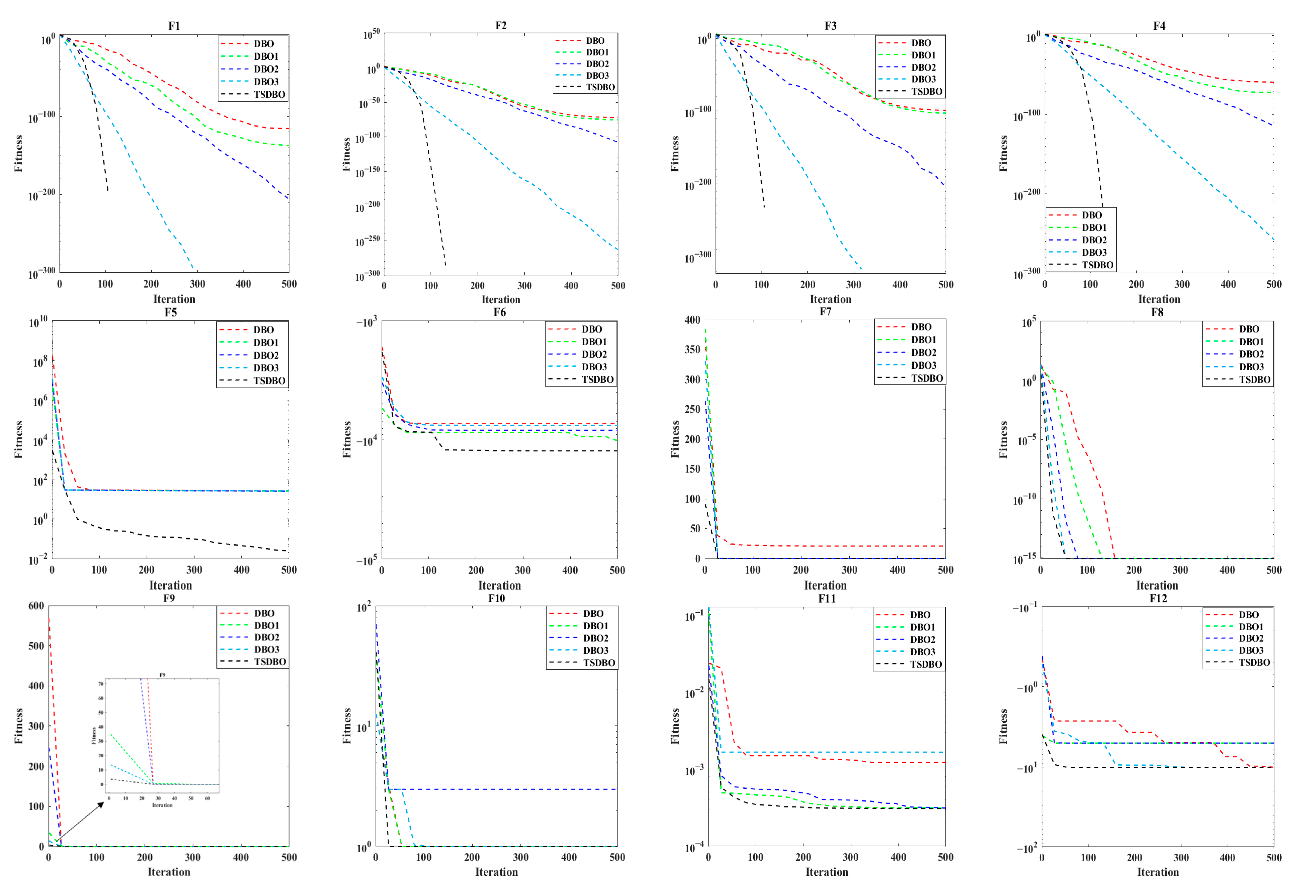
4.2. Analysis of the Effectiveness of Improvement Strategies

TSDBO includes three improvements to DBO, and three different algorithms are obtained by fusing DBO with these three kinds of improvements, respectively.

(1)

Adding the improved Tent chaotic mapping to initialize the population in DBO to obtain DBO1;

(2)

Introducing a dynamic spiral search strategy in DBO to obtain DBO2;

(3)

DBO is used with an adaptive t-distribution perturbation technique to produce DBO3.

The four algorithms of TSDBO with DBO, DBO1, DBO2, and DBO3 are experimented with the 12 test functions in Table 1. The optimization outcomes for 30 separate iterations of each algorithm, including the three metrics, are displayed in

Table 2. Comparison of different strategies.

Function	Index	DBO	DBO1	DBO2	DBO3	TSDBO
F1	Best	5.00 × 10−173	1.30 × 10−179	1.11 × 10−248	0	0
	Mean	7.19 × 10−108	6.50 × 10−116	4.32 × 10−206	0	0
	Std	3.94 × 10−107	3.56 × 10−115	0	0	0
F2	Best	1.66 × 10−81	4.27 × 10−84	4.57 × 10−121	9.59 × 10−280	2.48 × 10−288
	Mean	2.04 × 10−54	1.53 × 10−65	2.74 × 10−105	9.23 × 10−245	1.17 × 10−245
	Std	1.12 × 10−53	8.36 × 10−54	1.50 × 10−104	0	0
F3	Best	4.35 × 10−142	3.21 × 10−156	1.18 × 10−224	0	0
	Mean	2.82 × 10−88	4.75 × 10−85	3.87 × 10−182	0	0
	Std	1.02 × 10−87	2.58 × 10−84	0	0	0
F4	Best	5.06 × 10−88	7.92 × 10−83	6.28 × 10−120	1.30 × 10−285	1.38 × 10−289
	Mean	3.21 × 10−49	8.81 × 10−56	1.10 × 10−103	4.31 × 10−237	4.08 × 10−244
	Std	1.76 × 10−48	4.70 × 10−55	5.92 × 10−103	0	0
F5	Best	2.47 × 101	2.46 × 101	2.40 × 101	2.42 × 101	3.11 × 10−3
	Mean	2.51 × 101	2.51 × 101	2.44 × 101	2.48 × 101	3.52 × 10−1
	Std	2.20 × 10−1	1.81 × 10−1	1.67 × 10−1	1.81 × 10−1	1.02 × 10−1
F6	Best	−1.19E × 104	−1.25 × 104	−1.25 × 104	−1.25 × 104	−1.26 × 104
	Mean	−9.32 × 103	−1.06 × 104	−9.52 × 103	−9.41 × 103	−1.20 × 104
	Std	1.35 × 103	1.60 × 103	1.45 × 103	1.57 × 103	7.60 × 102
F7	Best	0	0	0	0	0
	Mean	1.99 × 101	1.26 × 100	0	0	0
	Std	4.80 × 101	6.03 × 100	0	0	0
F8	Best	8.88 × 10−16	8.88 × 10−16	8.88 × 10−16	8.88 × 10−16	8.88 × 10−16
	Mean	8.88 × 10−16	1.01 × 10−15	8.88 × 10−16	8.88 × 10−16	8.88 × 10−16
	Std	0	6.94 × 10−16	0	0	0
F9	Best	0	0	0	0	0
	Mean	2.74 × 10−4	3.24 × 10−3	0	0	0
	Std	1.53 × 10−3	1.62 × 10−2	0	0	0
F10	Best	9.98 × 10−1	9.98 × 10−1	9.98 × 10−1	9.98 × 10−1	9.98 × 10−1
	Mean	9.98 × 10−1	9.98 × 10−1	9.98 × 10−1	9.98 × 10−1	9.98 × 10−1
	Std	1.17 × 10−16	1.01 × 10−16	9.22 × 10−17	1.30 × 10−16	1.17 × 10−18
F11	Best	3.07 × 10−4	3.07 × 10−4	3.07 × 10−4	3.07 × 10−4	3.07 × 10−4
	Mean	7.36 × 10−4	7.84 × 10−4	6.19 × 10−4	7.97 × 10−4	3.37 × 10−4
	Std	3.36 × 10−4	3.94 × 10−4	3.93 × 10−4	4.67 × 10−4	6.40 × 10−5
F12	Best	−1.02 × 101	−1.02 × 101	−1.02 × 101	−1.02 × 101	−1.02 × 101
	Mean	−6.77 × 100	−7.09 × 100	−6.92 × 100	−9.98 × 100	−1.02 × 101
	Std	2.43 × 100	2.54 × 100	2.50 × 100	1.37 × 100	6.45 × 10−15

. Best indicates the algorithm’s correctness, while Mean and Std indicate its stability.

We can see from Table 2 and Figure 5 that DBO1, DBO2, and DBO3 have improved their optimization searching accuracy on most test functions compared to DBO, while TSDBO has improved on 11 test functions compared to DBO and 1 is comparable to DBO. Compared with DBO, DBO1, DBO2, and DBO3 have all three evaluation metrics improved to a large extent, where DBO2 and DBO3 are better than DBO1. This is due to the fact that DBO1 improves the quality of distribution of the initial populations across the search space by using only the improved Tent chaotic mapping, which raises the algorithm’s solution accuracy. The algorithm’s global optimal search performance can be improved by implementing the second technique, and at the same time, the algorithm’s optimization accuracy is somewhat enhanced based on the spiral characteristics, as demonstrated by the significant improvement in the optimal convergence value and average convergence accuracy on the 12 test functions when compared to DBO and DBO2. In contrast to DBO, DBO3 finds theoretically optimal values in the F1 and F3 functions. This is because the algorithm can now leap out of the local optimum when it enters it thanks to the introduction of the third approach, thereby improving algorithm performance. In comparison to DBO, TSDBO has substantially superior evaluation metrics, which integrates the three improved strategies, are improved compared with DBO, and the average convergence accuracy reaches the best value in F1, F3, F7, and F9 without negative optimization, which indicates that the integration of the three strategies is effective.

4.3. Comparison with Other Algorithms

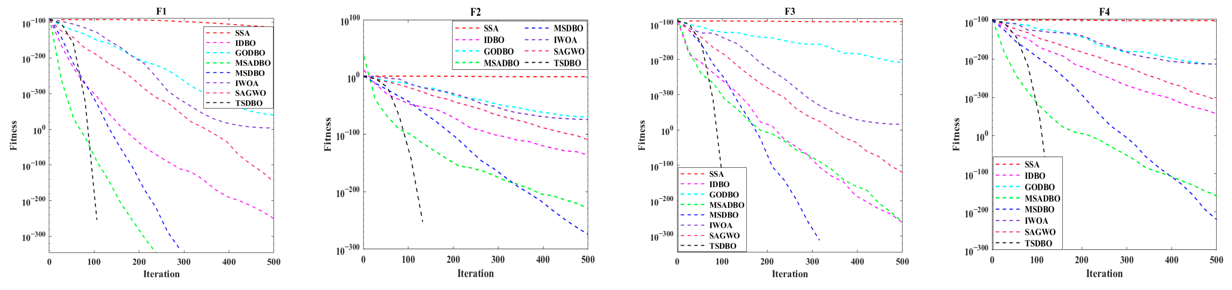
The TSDBO algorithm is compared against other enhanced algorithms in order to confirm its efficacy, including the Salp Swarm Algorithm (SSA) [41], the Dung Beetle Optimization Algorithm (IDBO) [42] with the introduction of a cycle mutation mechanism, the Multi-Strategy Dung Beetle Optimization Algorithm (GODBO) [43] based on Oppositional Learning (OBL), the Sinusoidal Algorithm–Directed Dung Beetle Optimization Algorithm (MSADBO) [44], the Multi-Strategy Improved Dung Beetle Optimization Algorithm (MSDBO) [45], the Improved Whale Optimization Algorithm (IWOA) [46], and the Gray Wolf Optimization Algorithm with Adaptive Search Strategy (SAGWO) [47]. The number of pertinent runs is still fixed at 500 iterations and 30 populations for the accuracy of the results. All algorithms’ other parameters were rigorously established in accordance with the original text. The optimization results of each method operating independently for 30 runs are displayed in

Table 3. Comparison with other algorithms.

Function	Index	SSA	IDBO	GODBO	MSADBO	MSDBO	IWOA	SAGWO	TSDBO
F1	Best	1.34 × 10−8	1.43 × 10−150	0	0	2.89 × 10−201	5.92 × 10−179	2.35 × 10−225	0
	Mean	2.24 × 10−8	3.56 × 10−114	2.34 × 10−164	0	3.02 × 10−185	1.85 × 10−111	1.34 × 10−214	0
	Std	6.79 × 10−9	1.95 × 10−113	0	0	0	1.01 × 10−110	0	0
F2	Best	2.60 × 10−2	1.19 × 10−81	8.42 × 10−28	2.71 × 10−268	2.64 × 10−232	1.32 × 10−84	2.01 × 10−126	6.30 × 10−279
	Mean	8.12 × 10−1	4.47 × 10−65	5.43 × 10−13	2.97 × 10−171	2.85 × 10−198	5.95 × 10−61	1.04 × 10−107	1.40 × 10−245
	Std	7.24 × 10−1	2.43 × 10−64	1.71 × 10−12	0	0	3.21 × 10−60	5.43 × 10−107	0
F3	Best	9.76 × 101	2.78 × 10−93	1.13 × 10−21	2.45 × 10−173	2.63 × 10−162	3.44 × 10−148	1.75 × 10−226	0
	Mean	5.47 × 102	1.48 × 10−46	8.54 × 10−11	8.81 × 10−111	7.89 × 10−132	5.70 × 10−27	5.21 × 10−178	0
	Std	4.56 × 102	7.28 × 10−46	3.69 × 10−10	4.83 × 10−110	5.62 × 10−142	3.12 × 10−26	0	0
F4	Best	2.60 × 100	4.19 × 10−73	5.85 × 10−19	9.06 × 10−259	8.54 × 10−245	7.02 × 10−75	2.98 × 10−126	2.30 × 10−286
	Mean	6.59 × 100	3.74 × 10-14	2.31 × 10−10	3.24 × 10−181	6.78 × 10−201	6.14 × 10−46	2.21 × 10−107	9.50 × 10−236
	Std	2.51 × 100	1.62 × 10-13	1.23 × 10−09	0	9.97 × 10−145	3.36 × 10−45	1.19 × 10−106	0
F5	Best	2.42 × 101	2.50 × 101	2.50 × 101	2.48 × 101	2.46 × 101	2.44 × 101	3.94 × 10-1	6.89 × 10−2
	Mean	1.44 × 102	2.58 × 101	2.56 × 101	2.55 × 101	2.57 × 101	2.50 × 101	2.36 × 101	2.34 × 10−1
	Std	3.50 × 102	3.47 × 10−1	2.30 × 10−1	3.33 × 10−1	3.50 × 10−1	2.17 × 10−1	4.38 × 100	7.04 × 10−2
F6	Best	−9.01 × 103	−1.03 × 104	−1.23 × 104	−1.23 × 104	−1.22 × 104	−1.14 × 104	−1.25 × 104	−1.26 × 104
	Mean	−7.57 × 103	−8.86 × 103	−8.34 × 103	−9.98 × 103	−9.99 × 103	−9.13 × 103	−1.00 × 104	−1.20 × 104
	Std	7.28 × 102	1.32 × 103	1.52 × 103	1.73 × 103	1.05 × 103	1.25 × 103	1.32 × 103	9.07 × 102
F7	Best	1.39 × 101	0	0	0	0	0	0	0
	Mean	3.87 × 101	1.56 × 100	1.85 × 100	9.45 × 10−1	0	4.88 × 100	0	0
	Std	1.43 × 101	3.24 × 100	1.83 × 100	5.63 × 10−1	0	2.14 × 101	0	0
F8	Best	2.89 × 10−5	8.88 × 10−16	8.88 × 10−16	8.88 × 10−16	8.88 × 10−16	8.88 × 10−16	8.88 × 10−16	8.88 × 10−16
	Mean	1.97 × 100	8.88 × 10−16	4.32 × 10−15	8.88 × 10−16	8.88 × 10−16	8.88 × 10−16	8.88 × 10−16	8.88 × 10−16
	Std	9.20 × 10−1	1.00 × 10−31	6.49 × 10−16	1.00 × 10−31	9.32 × 10−30	4.35 × 10−28	9.36 × 10−23	0
F9	Best	9.82 × 10−6	0	0	0	0	0	0	0
	Mean	1.06 × 10−2	1.94 × 10−3	2.05 × 10−4	1.98 × 10−4	1.95 × 10−4	2.01 × 10−4	2.55 × 10−4	0
	Std	1.03 × 10−2	4.58 × 10−3	5.21 × 10−3	6.32 × 10−4	5.36 × 1−-4	3.26 × 10−3	5.32 × 10−4	0
F10	Best	9.98 × 10−1	9.98 × 10−1	9.98 × 10−1	9.98 × 10−1	9.98 × 10−1	9.98 × 10−1	9.98 × 10−1	9.98 × 10−1
	Mean	1.23 × 100	2.57 × 100	9.98 × 10−1	1.20 × 100	1.54 × 100	1.06 × 100	1.26 × 100	9.98 × 10−1
	Std	5.01 × 10−1	2.92 × 100	4.52 × 10−1	6.05 × 10−1	5.32 × 10−5	3.62 × 10−1	3.26 × 10−2	1.37 × 10−15
F11	Best	3.08 × 10−4	3.07 × 10−4	3.07 × 10−4	3.07 × 10−4	3.07 × 10−4	3.07 × 10−4	3.07 × 10−4	3.07 × 10−4
	Mean	1.50 × 10−3	4.69 × 10−4	1.53 × 10−3	4.27 × 10−4	5.32 × 10−4	6.61 × 10−4	3.48 × 10−4	3.18 × 10−4
	Std	3.58 × 10−3	2.04 × 10−4	2.33 × 10−3	2.82 × 10−4	3.68 × 10−3	2.57 × 10−4	9.11 × 10−5	9.35 × 10−5
F12	Best	−1.02 × 101	−1.02 × 101	−1.02 × 101	−1.02 × 101	−1.02 × 101	−1.02 × 101	−1.02 × 101	−1.02 × 101
	Mean	−2.34 × 100	−1.00 × 101	−9.64 × 100	−4.42 × 100	−3.56 × 100	−6.69 × 100	−9.98 × 100	−1.02 × 101
	Std	3.56 × 101	3.90 × 10−1	1.56 × 100	1.70 × 100	2.10 × 100	2.53 × 100	9.31 × 10−1	6.56 × 10−15

along with the Best, Mean, and Std. To make it easier to read, TSDBO’s data have been bolded by us.

The TSDBO method reaches the theoretical ideal value of 0 in the F1-F3 functions. Out of the five single-peak benchmark functions (F1-F5), TSDBO performs better than the other six comparison algorithms in the F1-F4 function across all assessment measures. Finding the ideal value of single-peak functions is more challenging for the F5 function, and most functions’ optimal outcomes range around 25. According to Table 3’s statistics, the TSDBO algorithm’s optimization results can approach the F5 function’s optimal value, and its average value is lower than that of the other methods under comparison. The TSDBO method outperforms the seven algorithms in the comparison and ranks first out of the various algorithms when the combined overall performance of F1–F5 is taken into account.

In the four multi-peak benchmarking functions (F6-F9), the TSDBO can find the theoretical optimal value Best in F6, and the mean (Mean) is the smallest among several algorithms; in the F7 function, the TSDBO and MSADBO are tied for the first place. In the F8 function, the TSDBO and a number of additional algorithms are able to determine the theoretically ideal value, but the TSDBO’s Std value is smaller. In the F9 function, the TSDBO outperforms several other algorithms.

Various approaches can locate the optimum or the optimization results can be near the theoretical optimum in the three hybrid benchmark test functions (F10-F12). The TSDBO method outperforms a number of other algorithms in the F10 function, while its Std value is lower than the GODBO algorithm’s. The F11 function’s Best, Mean, and Std values are lowest for the TSDBO algorithm, which also has the greatest rating. All of the comparison algorithms discover the theoretically ideal value of Best in the F12 function; however, the TSDBO algorithm’s Mean and Std values outperform those of the other techniques.

(1)

Comparison between TSDBO and SSA: SSA is highly adaptive and can find optimal solutions on 12 test functions. However, the optimal solution found by SSA has a big gap compared with TSDBO, and the average value is much larger than TSDBO. And the standard deviation of SSA is larger than that of TSDBO, which is an indicator to reflect the stability of the algorithm, and a too-large standard deviation indicates that the deviation between the data is relatively large. The combined performance of the two algorithms indicates that TSDBO also has a good adaptive performance.

(2)

Comparison between TSDBO and IDBO: IDBO finds the optimal value in the F7 and F9 functions, but analyzing the data shows that IDBO improves the performance of the algorithm, but it is easy to fall into the local optimum, and it cannot be compared with TSDBO.

(3)

Comparison between TSDBO and GODBO: The performance of GODBO on the 12 test functions is average, even negative optimization occurs on some functions, and there is no competitive advantage compared with TSDBO.

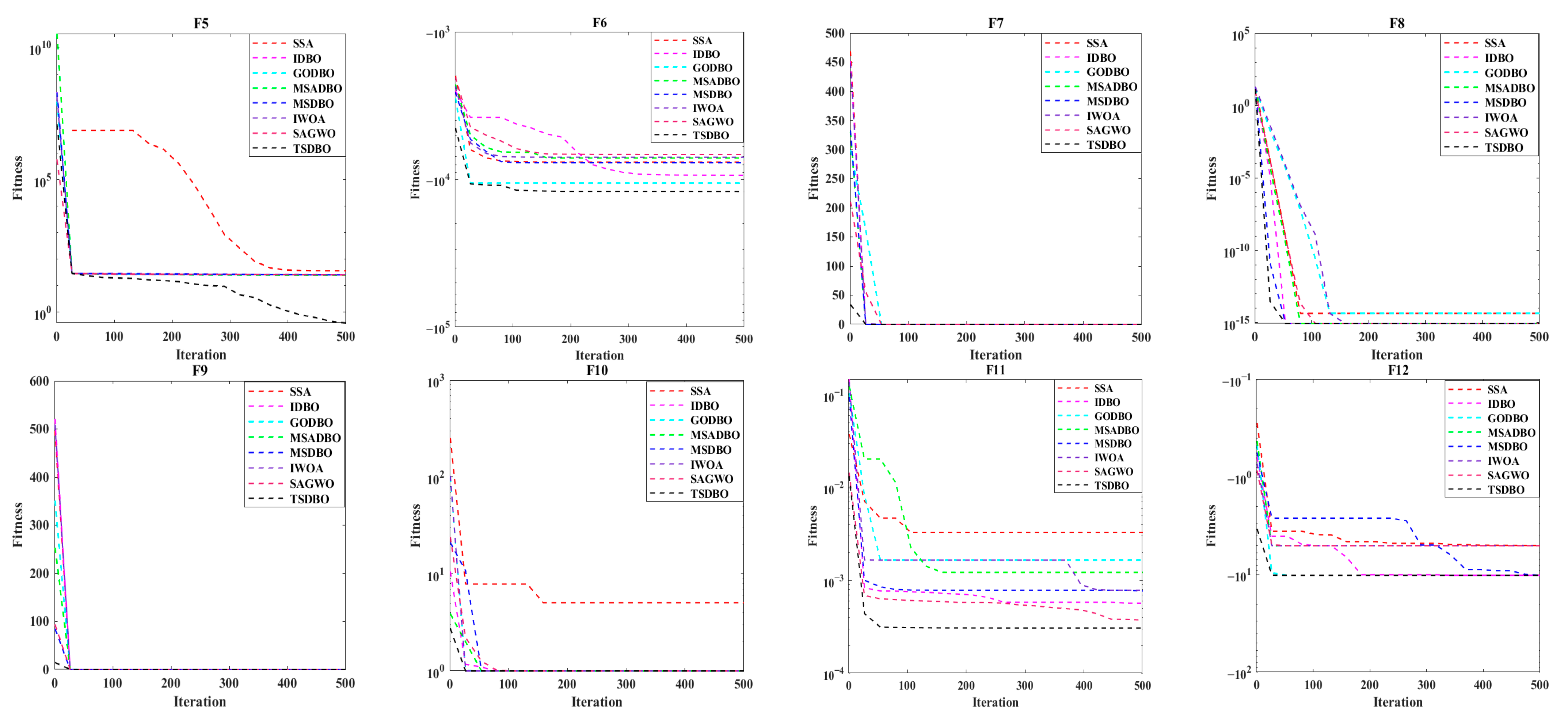
(4)

Comparison between TSDBO and MSADBO: The average convergence accuracy of TSDBO converges to the theoretical optimal solution on F1 and F3, while the average optimization accuracy of MSADBO only converges to the theoretical optimal solution on F1, and MSADBO, like most of the other optimization algorithms, falls into the local optimal solution in the function F5, where finding the best is more difficult, whereas the optimal value of TSDBO approaches the theoretical best value of 0, with an average convergence accuracy of 0. The theoretical optimal solution is 0, and the average convergence accuracy also reaches 2.34E−01, which is better than that of MSADBO; on the multi-peak functions F6-F9, TSDBO shows superior performance in searching for the optimal solution, which indicates that TSDBO is quite good at both local escape and global search; on the hybrid benchmark test functions F10-F12, the optimal values of TSDBO and MSADBO have the same optimal values, but are better than MSADBO in both average convergence accuracy and standard deviation. When analyzed together, TSDBO’s optimality-seeking performance on its test functions is stronger than MSADBO.

(5)

Comparison between TSDBO and MSDBO: Compared to IDBO and GODBO, MSDBO performs better overall, and it can find the theoretical best value in the F7 and F10 functions, but the Mean and Std are worse than those of TSDBO, and the optimization results are not as accurate as those of TSDBO on other functions.

(6)

Comparison between TSDBO and IWOA: IWOA performs similarly to GODBO on the test functions and has no competitive advantage over TSDBO.

(7)

Comparison between TSDBO and SAGWO: SAGWO outperforms GODBO and IWOA in F1-F4, has a good performance in the F6 function, and finds the theoretical optimal value in the F7, F9, and F10 functions, but the Mean and Std are not comparable to those of TSDBO, and the overall performance is not as good as TSDBO.

In summary, TSDBO has a decent performance in the comparison algorithms, with a combined performance of first place in each function. The introduction of the first strategy improves the initial population state of the algorithm and lays a solid foundation for the subsequent steps of the algorithm. The introduction of the second strategy improves the exploration and development of the algorithm dramatically, which can be explored more fully and the performance of the algorithm can be utilized. The introduction of the third strategy not only accelerates the convergence speed of the algorithm to a certain extent, but also allows the algorithm to jump out of the local optimum solution when it falls into the local optimum, so that the performance of the algorithm can be completely released.

To better help the reader understand the data in Table 3, we give the number of times each algorithm appears to be optimal in each metric in Figure 6. It can be clearly seen that TSDBO has the highest number of optimal times in each index, which means that TSDBO is ranked first in each algorithm. The second one is MSADBO and the third one is MSDBO. Other algorithms are not ranked because of their poor performance.

4.4. Convergence Curve Analysis

Figure 7 shows the iteration convergence curve of 12 test functions to more clearly illustrate each algorithm’s pace of convergence and capacity to avoid local optima. The following conclusions can be drawn from the information in Table 3 and Figure 7:

(1)

The TSDBO algorithm is the most accurate and fastest for functions F1–F4. In addition to determining the theoretically ideal values for functions F1 and F3, it also determines how many iterations are necessary to reach those values.

(2)

For function F5, while other algorithms become trapped in local optima, the convergence curve illustrates that the TSDBO algorithm outperforms them in both speed and accuracy. Moreover, the best value achieved by the TSDBO algorithm is close to the theoretical optimal value.

(3)

From the iteration convergence curve of functions F6–F9, it is evident that the TSDBO algorithm achieves faster convergence while maintaining high accuracy in the multi-peak benchmark functions. Unlike the comparison algorithms, it avoids repeated entrapment in local optima, showcasing its strong ability to escape local solutions.

(4)

In the hybrid benchmark functions F10–F12, Table 3 and Figure 7 show that TSDBO performs the best among the algorithms. This also confirms, side by side, that the algorithm is able to effectively balance the exploration and development capabilities of the algorithms.

It can be visualized in Figure 7 that the convergence speed and convergence accuracy of TSDBO rank first among several compared algorithms, which relies on the introduction of three improvement strategies. In the function with only the minimum value, TSDBO can converge quickly and find or approach the theoretical optimum, giving full play to the performance of the algorithm. In particular, in the F5 function, the convergence curve has an inflection point when falling into the local optimum, which is due to the fact that the third strategy will perturb the algorithm so that the algorithm jumps out of the local optimum and can continue to find the theoretical value. The hybrid function not only tests the convergence speed of the algorithm, but also requires the algorithm to have a good ability to explore and develop. In the hybrid function, TSDBO guarantees the convergence speed while still being far ahead of other comparison algorithms in terms of accuracy. TSDBO consistently outperforms in the 12 functions tested. On the multi-peak and hybrid functions, TSDBO is able to start the iterative optimization search from the neighborhood close to the theoretical value, which not only greatly reduces the number of iterations, but also enables the computer’s arithmetic power to be fully used. This is a good indication that the introduction of the three strategies is successful and can perform even better on top of the excellent performance of the base algorithm.

4.5. Robot Path Planning Based on TSDBO Algorithm

4.5.1. Environmental Modeling

When constructing the raster map, obstacles are processed based on their status to ensure they are properly formatted for display, facilitating efficient path planning. The higher the accuracy of the raster map, the better it reflects the original obstacle information. The processed raster map is shown in Figure 8, where the robot is able to move freely in the directions indicated in Figure 9. The robot’s start and end points must be white grids, or path planning cannot be accomplished. In Figure 8, the white grids represent open areas where the robot can navigate, while the black grids indicate obstacles that the robot cannot traverse. Assuming the position of the robot is M (i, j) the mathematical representation of the grid is provided in Equation (12).

$$M(i,j)=\left\{\begin{array}{c}0\hspace{1em}\hspace{1em}\left(\mathrm{Accessible} \mathrm{areas}\right)\hfill \\ 1\hspace{1em}\hspace{1em}\left(\mathrm{Obstacles}\right)\hfill \end{array}\right.$$

(12)

4.5.2. Constraints and Single-Objective Fitness Functions

In order to guarantee the feasibility of the path planning, a fitting function that fulfills the constraints must be created after the pertinent environmental data have been set up. The fitting function is linked to the following three requirements:

(1)

Path continuity. In path planning, the robot cannot appear to walk backwards. That is to say, if the robot starts from the starting point and its position at a certain point is (X1, Y1), then its next position should be (X2, Y2) and the condition X2 > X1 or Y2 > Y1 must be satisfied.

(2)

Limitations of obstacles and boundary conditions. In the path planning result, the robot’s moving path cannot appear to cross the boundary, and the search result cannot go beyond the boundary or pass through the area where obstacles exist in the grid.

(3)

Shortest path. If conditions (1) and (2) are satisfied, the path that retains the shortest path should be selected as the optimal path in robot path planning.

In summary, the single-objective fitness function can be described by Equation (13).

$$\cos \mathrm{t}i={\displaystyle {\sum }_{j=1}^{D-1}\sqrt{{\left(xj+1+xj\right)}^2+{\left(yj+1+yj\right)}^2}}$$

(13)

4.5.3. Two-Dimensional Map Model of 10 × 10

There are 20 iterations and a population size of 100 in the 10 × 10 map. DBO, GODBO, and MSADBO are selected as competitors. The optimal path for each algorithm in a 10 × 10 map is shown in Figure 10. To eliminate chance, each algorithm is run 10 times, and the average path, shortest path, longest path, and average time of each algorithm are recorded. From Figure 10, we can see that TSDBO has the shortest path, while DBO is clearly in the local optimum. As illustrated in

Table 4. The 10 × 10 robot path planning results.

Index	DBO	GODBO	MSADBO	TSDBO
Shortest Path	19.6569	19.3137	19.6569	18.2426
Longest Path	19.6569	24.4853	19.6569	19.6569
Average Path	19.6569	20.8752	19.6569	19.3740
Shortest Path time	3.95 s	3.45 s	8.99 s	5.02 s
Average time	4.88 s	3.62 s	9.44 s	5.41 s

, in terms of shortest path, average path, and longest path, TSDBO performs better than any other method. Although the TSDBO algorithm is a little longer than the DBO algorithm in terms of average time, these times are negligible considering the improvement of the optimization strategy. And the shortest path of TSDBO is 5.5% better than the shortest path of GODBO and 7.2% better than the shortest path of DBO and MSADBO. In Figure 11, when it comes to convergence speed and accuracy, TSDBO is the best.

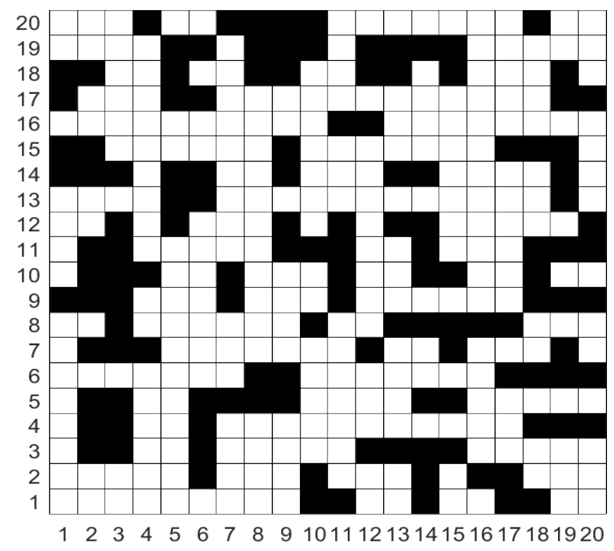
4.5.4. Two-Dimensional Map Model of 20 × 20

Additionally, there are 20 iterations and a population size of 100 in the 20 × 20 map. As competitors, DBO, GODBO, and MSADBO are chosen. Every algorithm operates on a 20 × 20 map, and Figure 12 displays the best course of action. Each method is performed ten times to remove chance, and the average time, shortest path, longest path, and average path are noted for each algorithm. From Figure 12, we can see that TSDBO has the shortest path, while DBO and MSADBO are clearly in the local optimum. As illustrated in

Table 5. The 20 × 20 robot path planning results.

Index	DBO	GOBDO	MSADBO	TSDBO
Shortest Path	36.9706	35.799	36.9706	31.5563
Longest Path	36.9706	49.2132	36.9706	36.9706
Average Path	36.9706	42.9647	36.9706	32.8436
Shortest Path time	11.87 s	10.38 s	26.20 s	11.30 s
Average time	13.24 s	10.99 s	28.15 s	11.98 s

, in terms of shortest path, average path, and longest path, TSDBO performs better than any other algorithm; also, its average time is less than DBO’s. When it comes to solving complex problems, the TSDBO algorithm performs better, demonstrating the effectiveness of the improvement strategy. Its shortest path improves by 11.9% over the shortest path of GODBO and by 14.6% over the shortest paths of DBO and MSADBO. Although the average time of GODBO planning paths is the shortest among several algorithms, its average path is the longest among several algorithms. In Figure 13, we can see the TSDBO plans the shortest path and is faster than the others. Therefore, the addition of multiple strategies allows the algorithm’s performance to be completely unleashed, which greatly improves the TSDBO’s ability to search and plan the optimal path.

5. Conclusions and Future Work

In this paper, we propose an enhanced version called TSDBO to improve the DBO algorithm. We adopt three major improvement strategies. In the early stage of TSDBO, the global search capability is enhanced by the improved Tent chaos mapping and dynamic spiral search. In the later stage, the local exploitation capability is enhanced by the adaptive t-distribution perturbation, which improves the search efficiency of the algorithm in the later stage. The three improvement strategies enhance the performance of the algorithm from the dimensions of population diversity, global exploration, and local exploitation, respectively. The algorithm’s total speed is increased by the focused enhancements at each stage, which allow it to easily identify the global optimal region and conduct effective searches within it.

In order to demonstrate the effectiveness of the strategy’s introduction, we evaluate TSDBO against a number of rivals in 12 benchmark functions. According to the experimental findings, TSDBO performs better than the original DBO and other rival algorithms. Additionally, TSDBO outperforms the competing algorithms in robot path planning, reducing the shortest path length by 5.5–7.2% on 10 × 10 2D maps and 11.9–14.6% on 20 × 20 2D maps. These results demonstrate the effectiveness and dependability of TSDBO in resolving practical issues in addition to confirming the strategy’s introduction.

Although TSDBO demonstrates excellent performance, the added optimization strategies increase processing time compared to the basic algorithm. However, in a complex 20 × 20 path planning environment, TSDBO reduces computation time and improves stability. The Dung Beetle Optimization Algorithm proposed in this study achieves better results in 2D path planning, but still suffers from the problem of locally optimal solutions. Future work will focus on the following directions: first, to address the local optimization problem of the algorithm, the global search capability of the algorithm can be further improved by adopting a more advanced adaptive mechanism. Second, considering that the current experiments are limited to static obstacle environments, the algorithm can be extended to dynamic obstacle environments in the future and combined with a real-time update mechanism to improve the dynamic adaptability of path planning. In addition, applying the improved algorithm to more complex 3D path planning problems and further verifying its performance in complex scenarios are important research directions in the future.

References

1. Faris, H.; Al-Zoubi, A.M.; Heidari, A.A.; Aljarah, I.; Mafarja, M.; Hassonah, M.A.; Fujita, H. An Intelligent System for Spam Detection and Identification of the Most Relevant Features Based on Evolutionary Random Weight Networks. Inf. Fusion 2018, 48, 67–83. [Google Scholar] [CrossRef]
2. Abbassi, R.; Abbassi, A.; Heidari, A.A.; Mirjalili, S. An efficient salp swarm-inspired algorithm for parameters identification of photovoltaic cell models. Energy Convers. Manag. 2019, 179, 362–372. [Google Scholar] [CrossRef]
3. Andi, T.; Huan, Z.; Tong, H.; Lei, X. A Modified Manta Ray Foraging Optimization for Global Optimization Problems. IEEE Access 2021, 9, 128702–128721. [Google Scholar]
4. Holland, J.H. Genetic Algorithms. Sci. Am. 1992, 267, 66–72. [Google Scholar] [CrossRef]
5. Storn, R.; Price, K. Differential Evolution—A Simple and Efficient Heuristic for global Optimization over Continuous Spaces. J. Glob. Optim. 1997, 11, 341–359. [Google Scholar] [CrossRef]
6. Xue, J.; Shen, B. A novel swarm intelligence optimization approach: Sparrow search algorithm. Syst. Sci. Control Eng. 2020, 8, 22–34. [Google Scholar] [CrossRef]
7. Mohamed, A.-B.; Reda, M.; Mohammed, J.; Mohamed, A. Nutcracker optimizer: A novel nature-inspired metaheuristic algorithm for global optimization and engineering design problems. Knowl. Based Syst. 2023, 262, 110248. [Google Scholar]
8. Jun, W.; Chuan, W.W.; Xue, H.X.; Lin, Q.; Fei, Z.H. Black-winged kite algorithm: A nature-inspired meta-heuristic for solving benchmark functions and engineering problems. Artif. Intell. Rev. 2024, 57, 98. [Google Scholar]
9. Naruei, I.; Keynia, F. Wild horse optimizer: A new meta-heuristic algorithm for solving engineering optimization problems. Eng. Comput. 2021, 38 (Suppl. S4), 3025–3056. [Google Scholar] [CrossRef]
10. Nitish, C.; Muhammad, M.A. Golden jackal optimization: A novel nature-inspired optimizer for engineering applications. Expert Syst. Appl. 2022, 198, 116924. [Google Scholar]
11. Shijie, Z.; Tianran, Z.; Shilin, M.; Mengchen, W. Sea-horse optimizer: A novel nature-inspired meta-heuristic for global optimization problems. Appl. Intell. 2022, 53, 11833–11860. [Google Scholar]
12. Agushaka, J.O.; Ezugwu, A.E.; Saha, A.K.; Pal, J.; Abualigah, L.; Mirjalili, S. Greater cane rat algorithm (GCRA): A nature-inspired metaheuristic for optimization problems. Heliyon 2024, 10, e31629. [Google Scholar] [CrossRef] [PubMed]
13. Shengwei, F.; Ke, L.; Haisong, H.; Chi, M.; Qingsong, F.; Yunwei, Z. Red-billed blue magpie optimizer: A novel metaheuristic algorithm for 2D/3D UAV path planning and engineering design problems. Artif. Intell. Rev. 2024, 57, 134. [Google Scholar]
14. Li, X.; Zhou, S.; Wang, F.; Fu, L. An improved sparrow search algorithm and CNN-BiLSTM neural network for predicting sea level height. Sci. Rep. 2024, 14, 4560. [Google Scholar] [CrossRef]
15. Sarada, M.; Prabhujit, M. Fast random opposition-based learning Golden Jackal Optimization algorithm. Knowl. Based Syst. 2023, 275, 110679. [Google Scholar]
16. Khattap, M.G.; Mohamed, A.E.; Ali, H.H.G.E.M.; Ahmed, E.; Mohammed, S. AI-based model for automatic identification of multiple sclerosis based on enhanced sea-horse optimizer and MRI scans. Sci. Rep. 2024, 14, 12104. [Google Scholar] [CrossRef]
17. Shen, J.; Hong, T.S.; Fan, L.; Zhao, R.; Ariffin, M.K.A.b.M.; As’arry, A.B. Development of an Improved GWO Algorithm for Solving Optimal Paths in Complex Vertical Farms with Multi-Robot Multi-Tasking. Agriculture 2024, 14, 1372. [Google Scholar] [CrossRef]
18. You, D.; Kang, S.; Yu, J.; Wen, C. Path Planning of Robot Based on Improved Multi-Strategy Fusion Whale Algorithm. Electronics 2024, 13, 3443. [Google Scholar] [CrossRef]
19. Knypiński, Ł. Constrained optimization of line-start PM motor based on the gray wolf optimizer. Eksploat. I Niezawodn. Maint. Reliab. 2021, 23, 1–10. [Google Scholar] [CrossRef]
20. Li, C.; Si, Q.; Zhao, J.; Qin, P. A robot path planning method using improved Harris Hawks optimization algorithm. Meas. Control 2024, 57, 469–482. [Google Scholar] [CrossRef]
21. Alejandro, P.C.; Daniel, R.; Alejandro, P.; Enrique, F.B. A review of artificial intelligence applied to path planning in UAV swarms. Neural Comput. Appl. 2021, 34, 153–170. [Google Scholar]
22. Jiankai, X.; Bo, S. Dung beetle optimizer: A new meta-heuristic algorithm for global optimization. J. Supercomput. 2022, 79, 7305–7336. [Google Scholar]
23. Bin, L.; Peng, G.; Ziqiang, G. Improved Dung Beetle Optimizer to Optimize LSTM for Photovoltaic Array Fault Diagnosis. Proc. CSU-PSA 2024, 36, 70–78. [Google Scholar]
24. Dong, S.; Zhenyu, Y.; Songbin, D.; Tingting, Z. Three-dimensional path planning of UAV based on EMSDBO algorithm. Syst. Eng. Electron. 2024, 46, 1756–1766. [Google Scholar]
25. Qin, G.; Qiaoxian, Z. Multi-strategy Improved Dung Beetle Optimizer and Its Application. J. Front. Comput. Sci. Technol. 2024, 18, 930–946. [Google Scholar]
26. Zhou, X.; Yan, J.; Yan, M.; Mao, K.; Yang, R.; Liu, W. Path Planning of Rail-Mounted Logistics Robots Based on the Improved Dijkstra Algorithm. Appl. Sci. 2023, 13, 9955. [Google Scholar] [CrossRef]
27. Jintao, Y.; Zhenhua, G.; Mingze, J.; Enqi, H. Robot path planning based on improved A* algorithm. J. Phys. Conf. Ser. 2023, 2637, 012008. [Google Scholar]
28. Quansheng, J.; Kai, C.; Fengyu, X. Obstacle-avoidance path planning based on the improved artificial potential field for a 5 degrees of freedom bending robot. Mech. Sci. 2023, 14, 87–97. [Google Scholar]
29. Wang, F.; Gao, Y.; Chen, Z.; Gong, X.; Zhu, D.; Cong, W. A Path Planning Algorithm of Inspection Robots for Solar Power Plants Based on Improved RRT*. Electronics 2023, 12, 4455. [Google Scholar] [CrossRef]
30. Lixing, L.; Xu, W.; Xin, Y.; Hongjie, L.; Jianping, L.; Pengfei, W. Path planning techniques for mobile robots: Review and prospect. Expert Syst. Appl. 2023, 227, 120254. [Google Scholar]
31. Gao, Y.; Li, Z.; Wang, H.; Hu, Y.; Jiang, H.; Jiang, X.; Chen, D. An Improved Spider-Wasp Optimizer for Obstacle Avoidance Path Planning in Mobile Robots. Mathematics 2024, 12, 2604. [Google Scholar] [CrossRef]
32. Gao, R.; Zhou, Q.; Cao, S.; Jiang, Q. Apple-Picking Robot Picking Path Planning Algorithm Based on Improved PSO. Electronics 2023, 12, 1832. [Google Scholar] [CrossRef]
33. Si, J.; Bao, X. A novel parallel ant colony optimization algorithm for mobile robot path planning. Math. Biosci. Eng. MBE 2024, 21, 2568–2586. [Google Scholar] [CrossRef] [PubMed]
34. Wahab, M.N.A.; Nazir, A.; Khalil, A.; Bhatt, B.; Noor, M.H.M.; Akbar, M.F.; Mohamed, A.S.A. Optimised path planning using Enhanced Firefly Algorithm for a mobile robot. PLoS ONE 2024, 19, e0308264. [Google Scholar] [CrossRef]
35. Huijun, L.; Ao, L.; Wenshi, L.; Ping, G. DAACO: Adaptive dynamic quantity of ant ACO algorithm to solve the traveling salesman problem. Complex Intell. Syst. 2023, 9, 4317–4330. [Google Scholar]
36. Tianrui, Z.; Wei, X.; Mingqi, W.; Xie, X. Multi-objective sustainable supply chain network optimization based on chaotic particle-Ant colony algorithm. PLoS ONE 2023, 18, e0278814. [Google Scholar]
37. Jiao, L.; Yong, W.; Guangyong, S.; Tong, P. Multisurrogate-Assisted Ant Colony Optimization for Expensive Optimization Problems with Continuous and Categorical Variables. IEEE Trans. Cybern. 2021, 52, 11348–11361. [Google Scholar]
38. Li, L.; Liu, L.; Shao, Y.; Zhang, X.; Chen, Y.; Guo, C.; Nian, H. Enhancing Swarm Intelligence for Obstacle Avoidance with Multi-Strategy and Improved Dung Beetle Optimization Algorithm in Mobile Robot Navigation. Electronics 2023, 12, 4462. [Google Scholar] [CrossRef]
39. Na, Z.; Zedan, Z.; Xiao-an, B.; Jun-yan, Q.; Biao, W. Gravitational search algorithm based on improved Tent chaos. Control Decis. 2020, 35, 893–900. [Google Scholar]
40. Mirjalili, S.; Lewis, A. The Whale Optimization Algorithm. Adv. Eng. Softw. 2016, 95, 51–67. [Google Scholar] [CrossRef]
41. Mirjalili, S.; Gandomi, A.H.; Mirjalili, S.Z.; Saremi, S.; Faris, H.; Mirjalili, S.M. Salp Swarm Algorithm: A bio-inspired optimizer for engineering design problems. Adv. Eng. Softw. 2017, 114, 163–191. [Google Scholar] [CrossRef]
42. Yazhong, Z.; Yigang, H.; Zhikai, X.; Kaixuan, S.; Zihao, L.; Leixiao, L. Power transformer vibration signal prediction based on IDBO-ARIMA. J. Electron. Meas. Instrum. 2023, 37, 11–20. [Google Scholar]
43. Zilong, W.; Peng, S. A Multi-Strategy Dung Beetle Optimization Algorithm for Optimizing Constrained Engineering Problems. IEEE Access 2023, 11, 98805–98817. [Google Scholar] [CrossRef]
44. Jincheng, P.; Shaobo, L.; Peng, Z.; Guilin, Y.; Dongchao, L. Dung Beetle Optimization Algorithm Guided by Improved Sine Algorithm. Comput. Eng. Appl. 2023, 59, 92–110. [Google Scholar]
45. Xin, K.; Bo, Y.; Hua, M.; Wensheng, T.; Hongfeng, X.; Ling, C. Multi-strategy improved dung beetle optimization algorithm. Comput. Eng. 2024, 50, 119–136. [Google Scholar]
46. Wu, Z.; Mu, Y. Improved whale optimization algorithm. Appl. Res. Comput. 2020, 37, 3618–3621. [Google Scholar]
47. Wei, Z.; Zhao, H.; Han, B.; Sun, C.; Li, M. Grey Wolf Optimization Algorithm with Self-adaptive Searching Strategy. Comput. Sci. 2017, 44, 259–263. [Google Scholar]
Figure 1. Logistic chaotic mapping.
Applsci 15 00396 g001
Figure 2. Tent chaotic mapping.
Applsci 15 00396 g002
Figure 3. Improved Tent chaotic mapping.
Applsci 15 00396 g003
Figure 4. Algorithm flowchart.
Applsci 15 00396 g004
Figure 5. Iteration convergence curve for different strategies and improved algorithm.
Applsci 15 00396 g005
Figure 6. Number of occurrences of the optimal indicator for each algorithm.
Applsci 15 00396 g006
Figure 7. Iteration convergence curve of various algorithms.
Applsci 15 00396 g007aApplsci 15 00396 g007b
Figure 8. Processed raster map.
Applsci 15 00396 g008
Figure 9. Robot movement direction.
Applsci 15 00396 g009
Figure 10. The 10 × 10 map path planning shortest path map.
Applsci 15 00396 g010
Figure 11. Convergence curve of 10 × 10 map path planning.
Applsci 15 00396 g011
Figure 12. The 20 × 20 map path planning shortest path map.
Applsci 15 00396 g012
Figure 13. Convergence curve of 20 × 20 map path planning.
Applsci 15 00396 g013