Article

The Application of Structural Reliability and Sensitivity Analysis in Engineering Practice

Faculty of Civil Engineering and Architecture, Kielce University of Technology, 25-314 Kielce, Poland
*
Author to whom correspondence should be addressed.
Appl. Sci. 2025, 15(1), 342; https://doi.org/10.3390/app15010342
Submission received: 7 October 2024 / Revised: 17 December 2024 / Accepted: 31 December 2024 / Published: 1 January 2025

Abstract

:
Standard safety assessments of civil engineering systems are conducted using safety factors. An alternative method to this approach is the assessment of the engineering system using reliability analysis of the structure. In reliability analysis of the structure, both the uncertainty of the load and the properties of the materials or geometry are explicitly taken into account. The uncertainties are described in a probabilistic manner. After defining the ultimate and serviceability limit state functions, we can calculate the failure probability for each state. When assessing structural reliability, it is useful to calculate measures that provide information about the influence of random parameters on the failure probability. Classical measures are vectors, whose coordinates are the first partial derivatives of reliability indices evaluated in the design point. These values are obtained as a by-product of the First-Order Reliability Method. Furthermore, we use Sobol indices to describe the sensitivity of the failure probability to input random variables. Computations of the Sobol indices are carried out using the classic Monte Carlo method. The aim of this article is not to define new sensitivity measures, but to show the advantages of using structural reliability and sensitivity analysis in everyday design practice. Using a simple cantilever beam as an example, we will present calculations of probability failure and local and global sensitivity measures. The calculations will be performed using COMREL modules of the STRUREL computing environment. Based on the results obtained from the sensitivity analysis, we can conclude that in the case of the serviceability limit state, the most significant influence on the results is exerted by variables related to the geometry of the beam under consideration. The influence of changes in Young’s modulus and load on the probability of failure is minimal. In further calculations, these quantities can be treated as deterministic. In the case of the ultimate limit state, the influence of changes in the yield strength is significant. The influence of changes in the load and length of the beam is significantly smaller. The authors present two alternative ways of designing with a probabilistic approach, using the FORM (SORM) and Monte Carlo simulation. The approximation FORM cannot be used in every case in connection with gradient determination problems. In such cases, it is worth using the Monte Carlo simulation method. The results of both methods are comparable.

1. Introduction

Sensitivity analysis is used to attain an in-depth understanding and categorization of the sources of uncertainty describing the loads and material parameters of a structure. The objective of this analysis is to ascertain the impact of these uncertainties on the structure’s response. Sensitivity analysis methods are fundamentally divided into local and global methods. Local sensitivity analysis methods [1,2,3] investigate the influence of altering a single random parameter on the structure’s response, specifically in the vicinity of a chosen point, typically the design point. Differential analysis methods dominate in this category. In this local method, sensitivity indices can be defined at a specific point in the probability space through the use of partial derivatives. The main disadvantage of local sensitivity analysis depends on the choice of the nominal point. Global sensitivity analysis methods focus on examining the behavior of a structure’s response influenced by any number of random parameters across the entire probability space. Currently, a number of measures have been suggested, which are widely used in engineering practice. In [4], the author describes the examination of scatterplots, regression analysis, correlation analysis, partial correlation analysis, statistical tests for patterns based on gridding, entropy tests for patterns based on gridding, nonparametric regression analysis, two-dimensional Kolmogorov–Smirnov test, and tests for patterns based on distance measures. Borgonovo, Chun, and Li [5,6,7] propose moment independent sensitivity indicators. A promising method for sensitivity analysis of models with uncertainty is also the Bayesian and Gaussian process method. Bayesian inference methods allow for updating probabilities based on new data and previous information. The introduction of Markov Chain Monte Carlo (MCMC) algorithms, such as Metropolis–Hastings and Gibbs sampling, made it possible to efficiently perform Bayesian inference on a large scale. MCMC algorithms allow for the generation of samples from posterior distributions, which is crucial for the practical application of Bayesian methods. In reliability analysis, Bayesian inference methods allow for updating initial assumptions about the limit function and parameters of the distributions, using information about the performance of the structure obtained at a later time. The use of Bayesian networks in sensitivity analysis is particularly valuable because it allows for the study of how changes in input values affect the model output in the context of uncertainty. Bayesian networks offer a flexible approach that takes into account both uncertainties in the data and dependencies between variables. In article [8] is proposed an enhanced Hierarchical Sparse Bayesian Learning (eHSBL) model for SHM field data forecasting and interpretation, correlation analysis, and uncertainty analysis. The proposed eHSBL model was used for the Tsing Ma Bridge (TMB), which is characterized by heterogeneities and high uncertainties. This interesting approach was successful in detecting and identifying damage for the SHM benchmark problem of Tianjin Yonghe Bridge [9]. In order to properly assess the structural performance of tall buildings, it is necessary to take into account uncertainties from various sources. In paper [10], the authors analyzed the seismic resistance of a 42-story building with a composite steel frame and a cast iron tubular core. In their research, they used a probabilistic method that takes into account various types of uncertainties. The uncertainties in the fragility analysis included the effects of loads, annual discount rate, cost index, and recovery time, as well as unknown parameters in the demand model. In this paper, the Bayesian updating rule is used to determine the posterior distribution of unknown parameters in the demand model. Based on the research, it can be concluded that taking into account the uncertainty of unknown parameters involved in the demand model has a significant impact on the estimation of fragility, expected costs, and seismic resistance of the structure. In [11], a hybrid AI-Bayes-based methodology is proposed for fragility estimation of tall buildings subjected to multiple earthquakes and winds. The proposed method is capable of fragility estimation to consider both epistemic and aleatoric uncertainties. The AI-Bayes-based method discussed in this paper provides great assistance in quantifying various uncertainties and improving the reliability of multi-hazard resilience assessment of tall buildings. Paper [12] presents the application of a hybrid Bayesian copula method to assess the wind-induced risk of tall buildings, taking into account various uncertainties. Bayesian theorem is used to develop posterior probability distributions of unknown parameters in the marginal probability distribution of wind speed and direction, as well as in the demand model for fragility estimates. On the other hand, the copula technique is used to develop a joint probability model of wind speed and direction. For this purpose, the corresponding marginal distributions of the variables discussed will be used. The application of this study shows that epistemic uncertainty has an obvious impact on both the probability of total damage based on deformation and comfort. Based on the collected results, we can conclude that the presented framework based on the Bayesian approach can well take into account the epistemic uncertainty related to unknown model parameters and random uncertainty.
Sobol and Iman [13,14,15] assess sensitivity via variance decomposition. Methods derived from the analysis of the variance of a structure’s response, after describing the model’s input uncertainties with appropriate probability distributions, can decompose the variance into components attributed to individual background variables and their combinations. The sensitivity of a structure’s response to changes in parameters is quantified by calculating the partial variance. Methods derived from variance analysis facilitate a comprehensive exploration of the input variables’ realization space, enabling the detection of all interactions within the computational model of the problem. Their use can be observed not only in civil engineering problems, but also in issues related to medicine.
Papers [16,17] are related to the modeling of systems containing implants used in abdominal hernia repair. Such models are often burdened with many uncertainties. In order to assess the influence of individual random variables, Sobolev indices calculated using the polynomial chaos expansion method were used. The polynomial chaos expansion is a method that allows approximation of the computational model using a series of multivariate polynomials. In [18], the authors developed a polynomial chaos expansion in mechanical problems, proposing a spectral stochastic finite element method. In many engineering problems, we can also use the polynomial chaos expansion method to calculate the global Sobol sensitivity indices [19,20]. In [21], efficient sampling methods are used to estimate the principal and total effect indices. For high failure probability, Monte Carlo simulation is derived to calculate sensitivity indices. In the case of small failure probability values, combined methods with importance sampling procedure and truncated importance sampling procedure are used to improve the computational efficiency. In [22], the relation of variance-based sensitivity measures to the directional cosines of the most probable failure point in an underlying independent standard normal space is discussed. Moreover, the authors point out the fact that there are one-to-one relations between them for linear limit state functions of normal random variables. The authors show that these discussed relations can provide a good approximation of variance-based sensitivities for general reliability problems.
Standard safety assessments of civil engineering systems are carried out using safety factors. An alternative method to this approach is the assessment of an engineering system using reliability analysis of the structure. In the reliability analysis of the structure, both the uncertainty of the load and the properties of the materials or geometry are taken into account explicitly. The uncertainties are described in a probabilistic manner. Once we have defined the ultimate and serviceability limit state functions, we can calculate the failure probability for each state. Additionally, we can check what impact individual random variables have on the probability of failure. We will use both local and global sensitivity measures for this purpose. Classical, local measures are vectors, whose coordinates are the first partial derivatives of reliability indices evaluated in the design point. These values are obtained as a by-product of the First-Order Reliability Method. In this paper, global sensitivity measures are Sobol indices. Computations of the Sobol indices are carried out using the classic Monte Carlo method. Of course, the calculation of Sobolev indices can be implemented in various ways, for example, using the polynomial chaos expansion method or advanced variance reduction methods. The key problem of using the polynomial chaos expansion method is the choice of regression points needed to calculate the coefficients. Widely used methods are Pure Random Sampling or Latin Hypercube Sampling. Unfortunately, these are computationally expensive methods. The Monte Carlo method is the optimal choice. It is not computationally expensive nor too demanding. The aim of this article is not to define new sensitivity measures, but to show the advantages of using structural reliability and sensitivity analysis in everyday design practice. Using a simple cantilever beam as an example, we will present the calculation of probability failure, additionally with local and global sensitivity measures. If the influence of a given random variable on the probability of failure is small, then, in further calculations, we can treat it as a deterministic variable. The calculations will be performed using COMREL modules of the STRUREL computing environment. The STRUREL computing environment was developed at the Technical University of Munich and has been developed and tested for over 30 years. STRUREL 2022 (V.13) is a modular software package. The main STRUREL modules are the following: COMREL (for reliability analysis of components), SYSREL (for reliability analysis of systems), COMREL-TV (for reliability analysis of time-dependent variables), COSTREL (for reliability optimization), and STATREL (for statistical data analysis). The software offers state-of-the-art numerical methods for structural reliability analysis.

2. Materials and Methods

When we define the problem of time-independent reliability analysis, we assume that the design parameters, whose values are characterized by uncertainty, are represented by an n-dimensional random vector X. In this research, realizations of random vector X in space Rn are described by vector x. Random parameters can be load multipliers, material constants (such as yield strength or Young’s modulus), or cross-section dimensions. Random vector X = {X1, X2, X3, …, Xn} takes values in the n-dimensional space of real numbers Rn. Reliability analysis assumes that a structure can be in one of two permissible states: either a safe state or a failure state. Failure can be understood as a failure to meet a constraint that has been imposed by the designer on the operation of the structure. In reliability analysis, this constraint is defined by a limit state function g(x). The limit state function is a function of vector X. If there is a joint probability density function f(x) for the random vector X = {X1, X2, X3, …, Xn}, then the failure probability Pf can be expressed by the following integral:
P f = P g x 0   P f = Ω f f x dx
where Ωf represents the failure area.
Calculating such a simple-looking integral in Formula (1) is very difficult in practice. The use of analytical methods is possible only in special cases. Standard methods of numerical integration also do not work. It is believed that quadrature can be used if the space of random variables has at most five dimensions. A popular method of integrating functions defined in a large number of dimensions is Monte Carlo simulation [23,24,25], together with variance reduction methods, for examples, Importance Sampling, Line Sampling, and Directional Sampling [26,27,28]. The First-Order Reliability Method (FORM) [29,30] and Second-Order Reliability Method (SORM) [31,32,33] approximation methods are also used to estimate the integral.
In assessing the reliability of building structures, the calculation of sensitivity measures is often used, providing information on the influence of input random variables on the probability of failure. Classical measures are vectors, whose coordinates are the first partial derivatives of reliability indices evaluated in the design point. These values are obtained as a by-product of the FORM. When a linear approximation of the limit function is insufficient, it is worth considering the SORM. This method is more time-consuming, which may cause problems when analyzing large engineering problems. It should always be remembered that the FORM gives the best results when there is only one design point, and the limit state function is not strongly non-linear and is differentiable. In case of problems with calculating the gradients of the limit state function, we cannot use the FORM. Then, we have to use one of the simulation methods in which we do not use gradient algorithms. This, of course, solves the problem of calculating the probability of failure, but we still cannot determine the sensitivity measures that are important to us. In this article, we will try to find an alternative solution using simple limit state functions. We will determine the sensitivity of the failure probability to input random variables using the analysis of variance of the characteristic function of the failure area. We will show the possibilities of calculating various measures of sensitivity on the example of a cantilever beam. We will formulate the ultimate and serviceability limit state functions. For each function, we will calculate the corresponding failure probability using two different methods, i.e., the FORM (SORM) and Monte Carlo. Additionally, in each method we will calculate qualitatively different sensitivity measures. In the case of the FORM, these will be the previously mentioned measures of elasticity of the reliability index, in the case of the Monte Carlo method, the Sobolev index. In the final part of the analysis, we will compare the failure probability sensitivity measures obtained using the two different methods.

2.1. First-Order Reliability Method—FORM, Hasofer–Lind Reliability Index

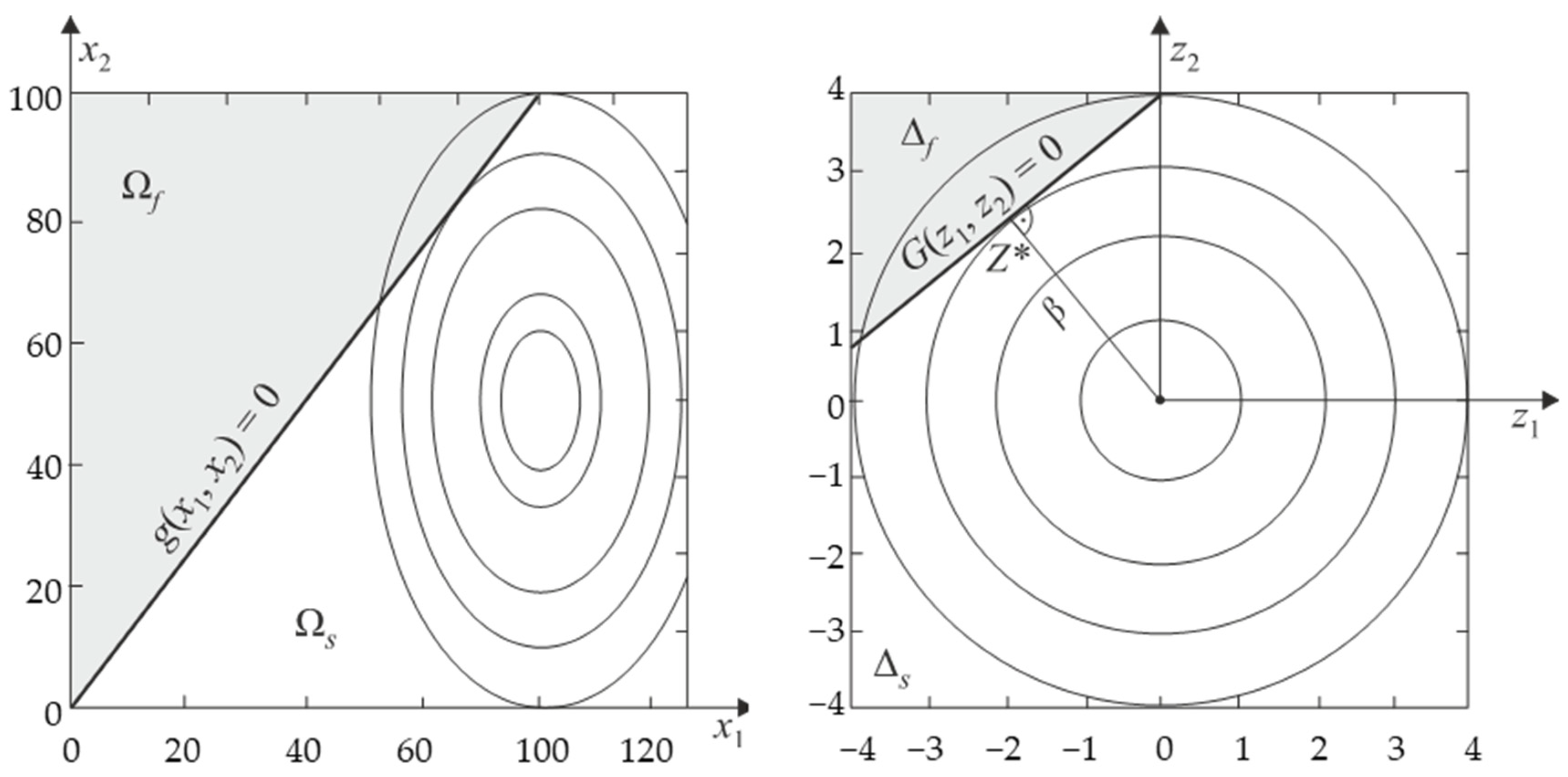
Consider the limit state function g(X1, …, Xn) in which the random variables are uncorrelated and normally distributed (Figure 1).
The limit state function can be represented in the standard form of random variables as follows:
Z i = X i - μ X i σ X i and X i = μ X i + Z i σ X i
Replacing X1, …, Xn with standard variables Z1, …, Zn, we obtain a new limit state function G(Z1, …, Zn).
The Hasofer–Lind reliability index β is defined as the shortest distance from the origin in the space of standard random variables to the boundary delineated by the equation G(Z) = 0. This definition means that in practice, β is the shortest distance from the point (0, …, 0) to the n-dimensional surface G(Z1, …, Zn) = 0 (Figure 2). The point located on the G(Z1, …, Zn) = 0—surface is called the design point, and its coordinates are denoted as ( Z 1 * ,   ,   Z n * ). Therefore, the following formula can be used to determine the reliability index:
β = i = 1 n Z i * 2
The value of the joint probability density function that corresponds to the failure at this point is the largest, due to the properties of the standard Gaussian space. This point reflects the most probable failure location among all points in this area.
To perform the calculations, the iterative method can be used, which consists in solving the system of (2n + 1) equations with (2n + 1) unknowns: β ,   α 1 ,   α 2 ,   ,   α n ,   Z 1 * ,   Z 2 * ,   ,   Z n * . The set of equations encompasses the relationships described by Formulas (4)–(7):
G Z 1 * ,   ,   Z n * = 0
Z i * = β α i
i = 1 n α i 2 = 1
α i = G Z i d e s i g n p o i n t i = 1 n G Z i d e s i g n p o i n t 2
The iterative procedure algorithm can be divided into the following steps:
  • Define the limit state function and determine the corresponding parameters of the distributions of the random variables Xi.
  • Find the initial design point { X i * } by assigning initial values to n − 1 variables Xi (mean value consideration is often used). Solve the equation g(X) = 0 with respect to the remaining random variable. This ensures that the initial point belongs to the boundary of the failure area.
  • Determine the values of the standard variables { Z i * } that correspond to the design point:
    Z i * = X i * μ X i σ X i
  • Determine the partial derivatives of the limit state function with respect to standard random variables. The column vector {K} should be defined as follows:
    K = K 1 K 2 . . . K n where   K i = G Z i d e s i g n p o i n t
  • Calculate the approximation β using the formula below:
    β = K T { Z * } K T { K } ,   where   Z * = Z 1 * Z n * . . . Z n *
  • Calculate the column vector of sensitivity coefficients:
    α = { K } K T { K }
  • Determine a new design point in the space of reduced random variables for n − 1 variables:
    Z i * = β α i
  • Determine the corresponding design point in origin coordinates for n − 1 variables from step 7:
    X i * = μ X i + Z i * σ X i
  • Calculate the values of the remaining random variable (i.e., undefined in steps 7 and 8) by solving the equation g(X) = 0. Steps 3–9 are repeated until β and the coordinates of the design point { X i * } converge.
The Hasofer–Lind reliability index is originally defined for the case when the distributions of random variables are unknown (we assume only normal distributions). In the case when the distributions are known, then β can be calculated using the Rackwitz–Fiessler method [29]. For this case, it is required to know the cumulative distribution function FX(X), and the probability density function fX(X) of the random variables present in the limit state function. Nonnormal distributions are replaced by normal distributions so that the cumulative distribution functions and probability density functions have the same value for the true and surrogate distributions at the design point. For each random variable X, two equations with two unknowns ( μ X e and σ X e ) can be written:
F X X * = Φ X * μ X e σ X e f X X * = 1 σ X e φ X * μ X e σ X e
After solving the system of equations, the following standard deviation of the surrogate normal distribution:
σ X e = 1 f X X * φ Φ 1 F X X *
and the following mean value of the surrogate normal distribution:
μ X e = X * σ X e Φ 1 F X X *
are obtained.
In the next steps, we proceed according to the algorithm described above.
Determining the correct design point is one of the most important issues for determining the correct value of the reliability index. There are many developed algorithms for calculating the design point. The articles by Hasofer and Lind [30] and Rackwitz et al. [31] are based on gradient methods, which, due to slow convergence, and in cases involving highly non-linear boundary surfaces, even no convergence, were identified as a limitation of the procedure. The incorporation of the step-length reduction procedure proposed by Abdo [34] into the Rackwitz–Fiessler algorithm partially solves this problem. An alternative to this approach is the sequential quadratic programming (SQP) algorithm developed by Schittkowski [35,36,37] and Arora [38]. They use additional information about the second derivatives to determine the search direction. In practice, this information is obtained by approximating the Hessian matrix of the Lagrange function only with gradients. The most commonly used Hessian approximation method is the BFGS (Broyden–Fletcher–Goldfarb–Shannon [31]) method. Paper [39] presents the possibility of using the FORM to assess the reliability of the optimized structure.

2.2. Monte Carlo Method

The Monte Carlo method was developed by John von Neumann’s team during World War II, while working on nuclear weapons at Los Alamos. Von Neumann utilized the simulation approach to describe the random nature of neutron diffusion. The Monte Carlo method has long been recognized as the technique with the highest accuracy of all methods requiring knowledge of the probability distribution of random parameters [40].
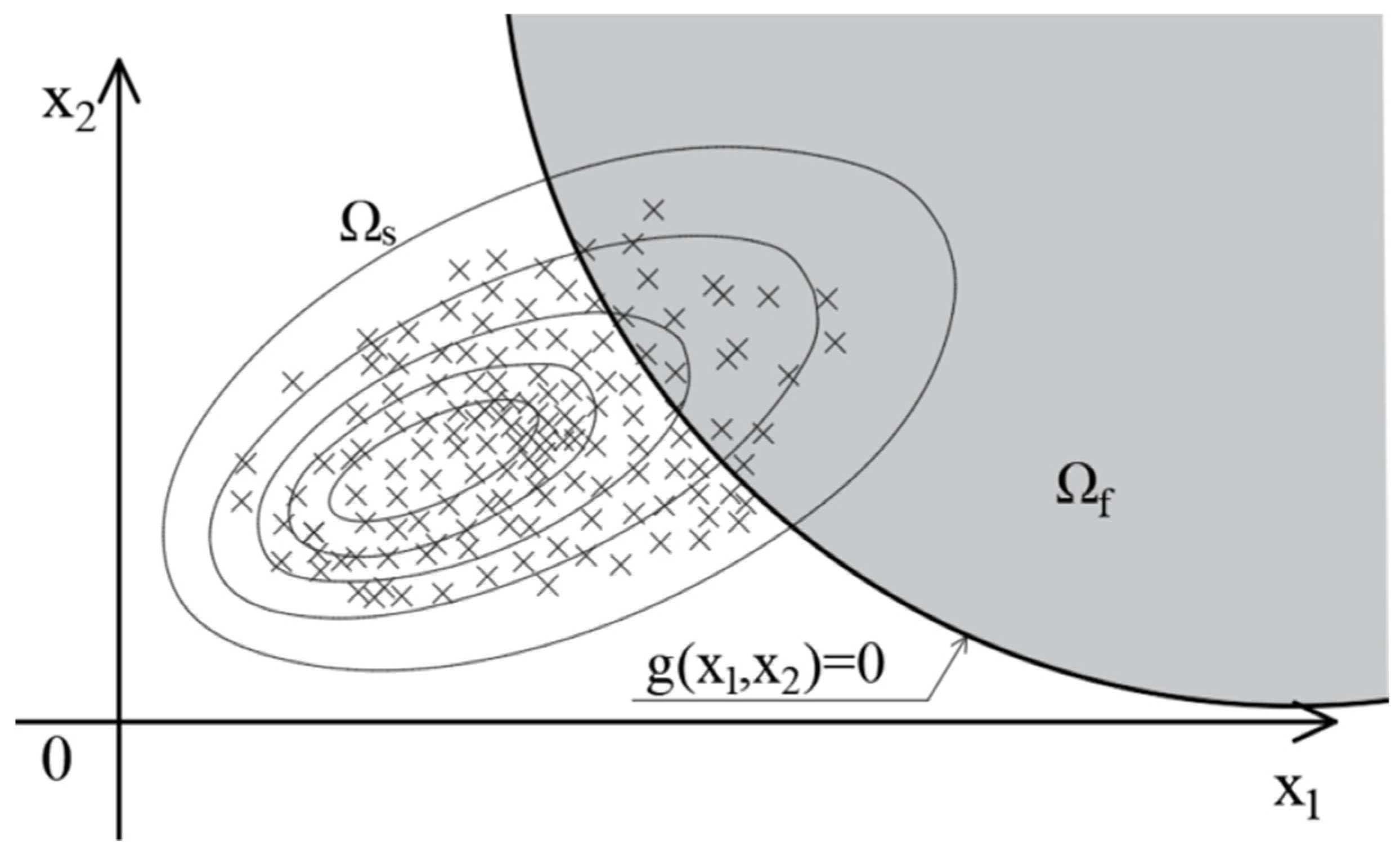
The Monte Carlo method utilizes statistical analysis of a random sample obtained from the simulation to solve the problem. The method is commonly used for numerical integration of functions of multivariate random variables; estimation of failure probabilities also belongs to this class of problems. An approximation of the probability of failure is obtained from an estimate of the expected value of the characteristic function of the failure area, obtained using an estimator appropriate for the simulation method adopted. The classical Monte Carlo simulation involves generating a realization of x of a random vector X, according to the joint probability distribution density fX(x), and then checking whether the realization lies in the safe area or in the failure area. We define the failure probability estimator as the number of “hits” in the failure region relative to the total number of simulations (Figure 3).
The above concept can be written down by defining the characteristic function of the set (failure area) as follows:
I Ω f X = 1 i f   X Ω f 0 i f   X Ω f
It is easy to see that each simulation involving the determination of I Ω f X values corresponds to a single realization of the Bernoulli test. The number of unreliable states in K attempts can be considered as a random variable with a binomial distribution:
P I Ω f X = 1 = P f P I Ω f X = 0 = 1   P f
where P f = P [ X Ω f ] .
The expected value and variance of I Ω f X take the form the following, respectively:
E I Ω f X = P f + 0 1     P f = P f
Var I Ω f X = E I Ω f X 2 E I Ω f X 2 = P f P f 2 = P f 1   P f
The Monte Carlo method uses an estimator of the mean value of the failure area characteristic function of the form to calculate the probability of failure:
1 K k = 1 K I Ω f X k = P f ~
where Xk are independent random vectors with a probability distribution defined by the density function fX(x), and K is the number of simulations.
The mean value and variance of the estimator are given, respectively, as follows:
E P f ~ = E [ 1 K k = 1 K I Ω f X k ] = 1 K KE [ I Ω f X ] = 1 K K P f = P f
Var P f ~ = Var 1 K k = 1 K I Ω f X k = 1 K 2 V a r [ k = 1 K I Ω f X k ] = 1 K 2 K   V a r [ I Ω f X ]   = 1 K 2 K P f 1     P f =   1 K P f 1   P f
The coefficient of variation of the estimator take the form of the following:
v P f ~ = σ P f ~ P f 0 ~ = 1     P f K P f
The above formula shows that obtaining a coefficient of variation of the estimator of 0.1 with a predicted probability of failure, which for real designs ranges from 10−7 to 10−4, requires K = 106–109 simulations, which, even with the capabilities of today’s multiprocessor computers, is an overwhelming task, if at all feasible in an acceptable time.
An alternative to determining the point estimator, together with its error, is to determine the so-called confidence interval in which, with the assumed confidence level, the probability of failure Pf is contained. We can determine the confidence interval of the estimator (20) using the information of the following random variable:
Y k = 1 K k = 1 K I Ω f X k E [ I Ω f X ] v P f ~
based on the central limit theorem that has an asymptotically standard normal distribution N(0,1). If C is the assumed confidence level, and kC is the quantile of the distribution N(0,1) of order ½(1 − C), then for n → ∞, the following relationship occurs:
P k c Y k k c = C
Having an estimate of the probability of failure (20) and an estimate of its variance (22), an approximation of the confidence interval of the probability of failure is obtained:
P P f ~ + k c v P f ~ p f P f ~ k c v P f ~ = C
The classic Monte Carlo method in reliability analysis uses simulations from the probability distribution of random parameters of the structure. The probability of failure can also be estimated based on samples from other probability distributions. It turns out that the appropriate selection of the probability distribution for the problem being solved allows one to significantly reduce the number of simulations needed to obtain an estimate of the required accuracy. The method using this approach is called Importance Sampling [41,42,43]. Shifting the mean value of the probability distribution to the design point, from which a random sample is generated, is the most commonly used strategy of the Importance Sampling method in reliability analysis. Based on the above formula, the failure probability estimator P f ~ takes the following form:
P f ~ = 1 K k = 1 K I Δ f ( W k ) φ n ( W k , 0 , I ) g w W k
where the realizations wk of vector Wk generated according to the probability distribution given by gw(w) are used to calculate the estimator.
An interesting extension of the Importance Sampling method is Line Sampling and Directional Sampling. In the Line Sampling method, samples are generated on a hyperplane tangent at the design point to the boundary surface. The coordinate system v is chosen so that the hyperplane passing through the design point is perpendicular to the first Cartesian coordinate. The origin of the coordinate system v is the same as the origin z. Therefore, the sampling space is rotated and reduced by one dimension. Let f(v) denote the probability density function that is used to generate these samples. Typically, f(v) is chosen as the standard normal distribution for v2, v3, …, vn, where n is the total number of random variables. The coordinate v1 is zero for all samples, since the samples should lie on the hyperplane. Then, for each sample v1 from f(v), we find the distance of the boundary surface perpendicular to the hyperplane. This distance is denoted as d(vi). In this case, the probability of failure is estimated from the samples as follows:
P f ~ = 1 n i = 1 n Φ [ - d v i ]
The Directional Sampling method expresses a random sample z as a point on a hypersphere of radius r. Any sample z can be uniquely expressed in terms of radius r and n − 1 direction angles αj, where n is the total number of random variables, and j = 1, …, n − 1. Let r and the direction angles αj be realizations of random variables denoted R and Aj, respectively. To generate samples that conform to the standard multivariate normal distribution, the variables Aj must be uniformly distributed random variables, and the random variable R2 must have a chi-square distribution with n degrees of freedom. The idea of directional sampling is to first generate a random direction using the direction angles αj, and then, using gradientless methods, search the line in the generated direction to find a point for which the limit state function takes the value zero. The distance of this point from the origin is denoted as ri. Based on the total number of N samples, the probability of failure Pf can be approximated as follows:
P f ~ = 1 n i = 1 n [ 1 χ n 2 ( β i 2 ) ]
where χ2 is the CDF of the chi-square distribution with n degrees of freedom.
This method can handle problems that have multiple (local) design points or if the failure is defined as a combination of different failure modes. However, directional sampling is not suitable for problems with multiple random variables. Interesting comments on this topic are given in [26,27,28,44,45].

2.3. Sensitivity Measures of Probability of Failure

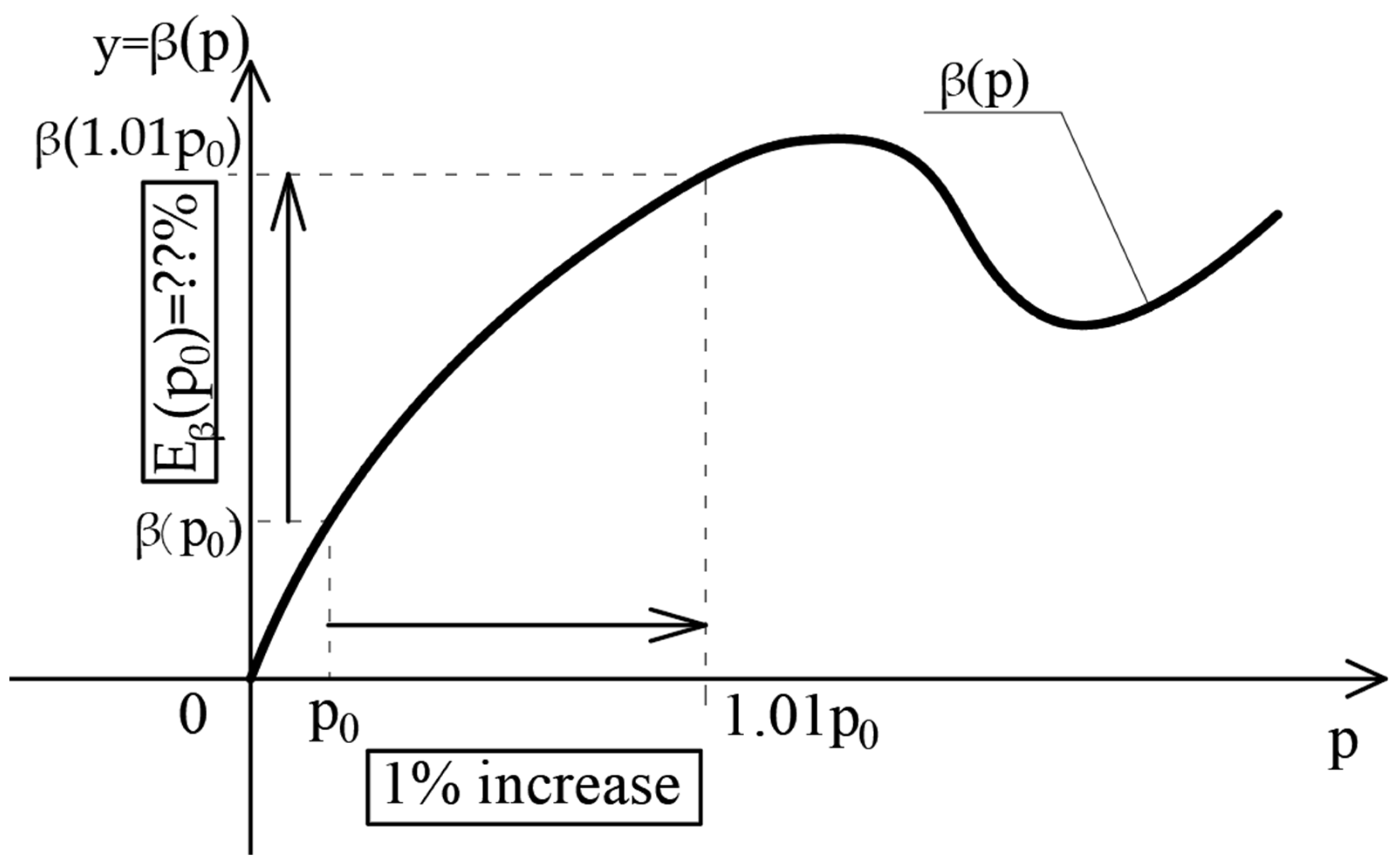
During the assessment of the reliability of building structures, it is important to determine the measures that can provide information about the influence of input random variables on the probability of failure. Classical measures include the coordinates of the vector α, obtained as a by-product of the first-order reliability method (FORM), and the elasticity of the reliability index (Figure 4).
The sensitivity of the reliability index to the coordinates of the design point Z* takes the following form:
β Z i z = z * = α i , i = 1 , , n
The vector α is often interpreted as a relative measure of the importance of individual standard variables. Higher values of the parameter αi indicate a higher sensitivity of β to the coordinate variable Zi. Negative values of αi mean that an increase in the coordinate Zi will cause a decrease in the reliability index β. On the other hand, positive values of the parameter αi are defined as an increase in the reliability index with an increase in the coordinate Zi. A correct understanding and interpretation of the sensitivity of the reliability index is helpful in predicting trends in the optimization process and building a stochastic model. In order to better compare the obtained sensitivity values, it is possible to include a standardized measure of sensitivity, the so-called elasticity of the reliability index, in the following form:
E β p i = β p i p i β
where Eβ is the percentage change of β with a 1% change in parameter pi. Parameter pi can be the expected value or standard deviation of a random variable. Respectively, they can be written as follows
E β σ i = β σ i σ i β
E β X i ¯ = β X i ¯ X i ¯ β
Taking into account the elasticity vector in the analyses allows for reducing the number of random variables in the description of the structure. Low values of the elasticity index resulting from the standard deviation of the variable Xi suggest that the influence of Xi on the failure probability value can be considered small, and the given quantities can be treated as deterministic in further calculations.
However, it should be remembered at all times that the FORM gives the best results with a single design point, where the limit state function is not strongly non-linear and is differentiable. If problems arise in calculating the gradients of the limit state function, the use of the FORM becomes impossible. In such cases, one must resort to using simulation methods that do not rely on gradient algorithms. While this is a viable solution for calculating the probability of failure, it does not provide the ability to determine significant sensitivity measures. We attempt to find an alternative solution using a simple limit state function. The sensitivity of the probability of failure to the input random variables will be determined using the analysis of variance of the failure area characteristic function I Ω f X (Formula (30)). The expected value and variance of this function are known (Formulas (32) and (33)). The probability of failure formula is presented below:
P f = Ω f f x d x = R n I Ω f x f ( x ) d x = E [ I Ω f X ]
In order to simplify the notation of the following mathematical formulas, Y = I Ω f X :
Y X = f 0 + i M f i X i + i < j M f i j X i , X j + + f 1 M X 1 , , X M
where f0 = E(Y) and E [ f i 1 i s ( X i 1 , , X i s ) = 0 for each subset of X i 1 , , X i s .
The variance of the function Y is presented as the sum of the variances Vi and Vi,j:
Var Y = i = 1 M V i + i = 1 M V ij + + V 1 M
where V i = Var E Y X i , and V ij = Var E Y X i , X j V i V j .
First-order Sobol indices Si and second-order indices Sij are defined as follows:
S i = V i Var Y S ij = V ij Var Y
For the Sobol indices Si and Sij, the following relationship occurs:
i M S i + i < j M S ij + + S 1 M = 1  
The total Sobol index STi is expressed by the following formula:
S T i = E V a r E Y X ~ i V a r Y = 1 = V a r E Y X ~ i V a r Y i M S T i 1
Var(Y) is known when calculating Sobol indices using the Monte Carlo method:
V a r I Ω f X = V a r Y = P f ( 1 P f )
The first-order Sobol index assesses the effect of changing Xi to the Y function. Interactions with other model input variables are not taken into account during the calculation. These interactions are included in the total Sobol index, which will not be analyzed in this example. Sensitivity measures based on Sobol indices [13,14] can be seen as an extension of variance-based sensitivity analysis. The first-order indices indicate the proportion of variance of the individual components of the X vector and can be regarded as a modified version of the moment-independent measure of failure probability sensitivity. The higher order and total effect indices represent the combined contribution of the components of vector X.

3. Case Study

The possibilities of calculating various sensitivity measures in reliability analysis will be presented using the example of a cantilever beam. For this purpose, a beam with a length l = 150 cm, a square tube-shaped section with dimensions D = 8.0 cm and d = 6.0 cm, Young’s modulus E = 21,000 kN/cm2, Poisson’s ratio v = 0.3, and yield strength fy = 23.5 kN/cm2 is used. The beam load was assumed to be uniformly distributed with an intensity of q = 0.06 kN/cm, as shown in Figure 5. The values are the mean values of the random variables D, d, E, q, l, fy (Table 1).
Random variables are described by a normal distribution. Correlations between random variables were not included in the calculations.
The vertical displacement of the cantilever end was computed according to the rules of statics as w = q   l 4 8   E   I , where I = D 4 d 4 12 .
The serviceability limit state function was defined as the condition of not exceeding the permissible vertical displacement wd = 1 cm:
f S LS X =   w d q l 4 8 E I
The reliability index and probability of failure were calculated using the FORM and SORM (Table 2).
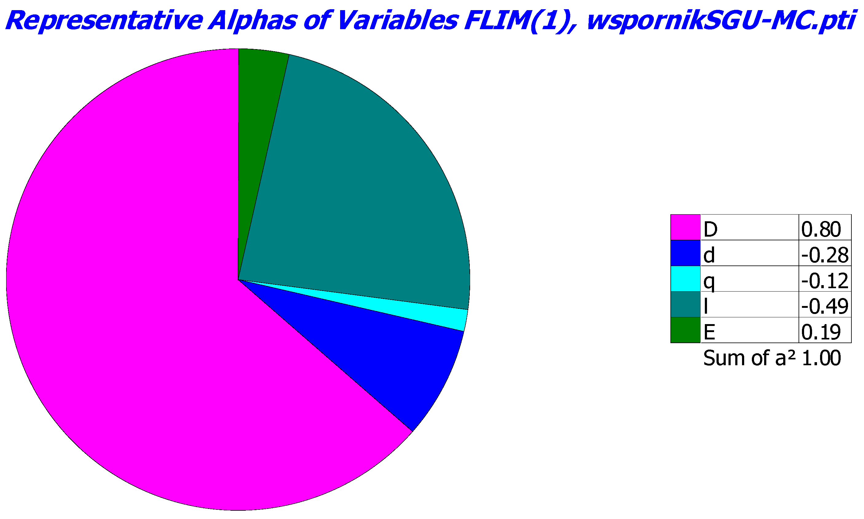
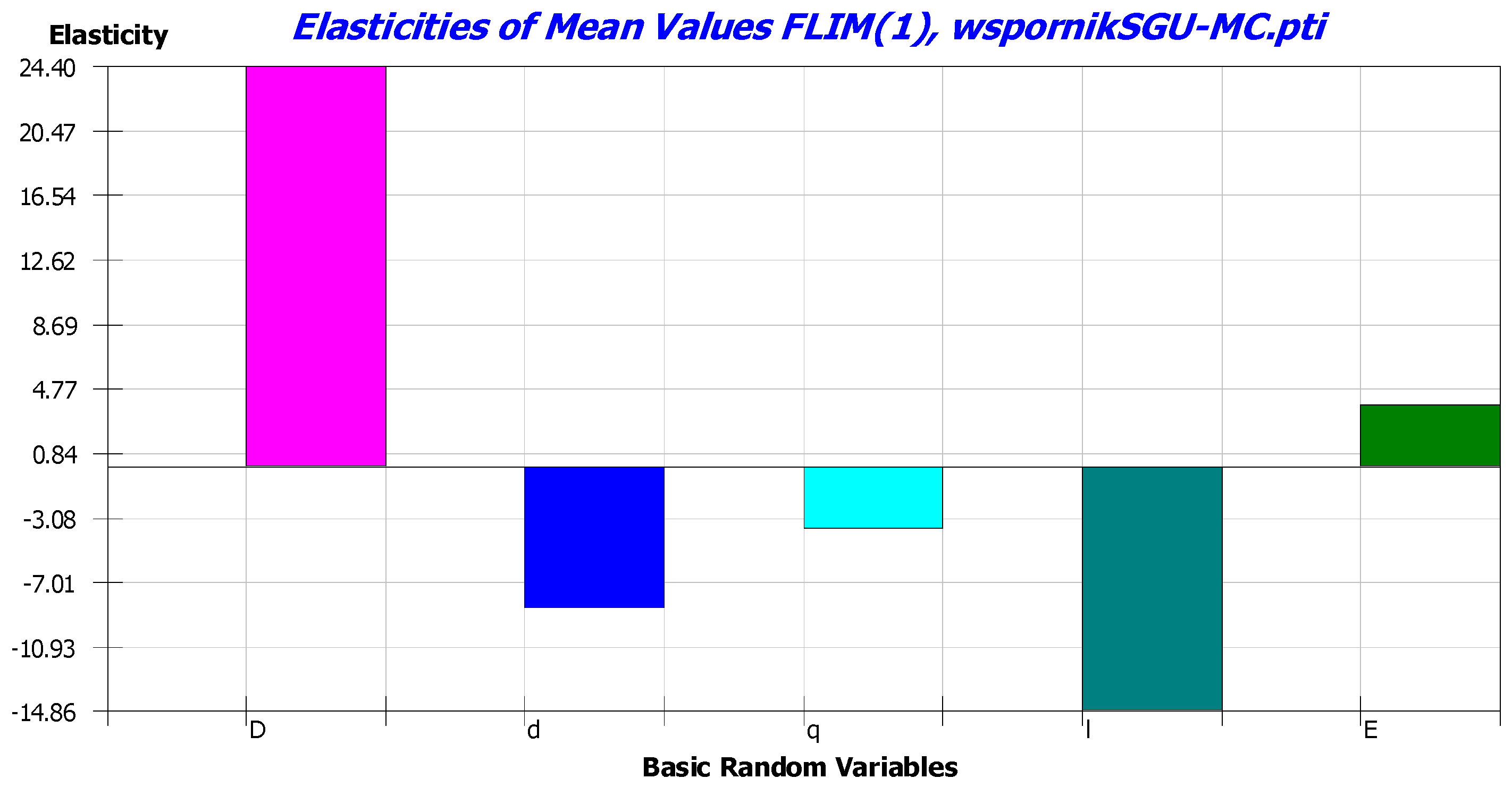
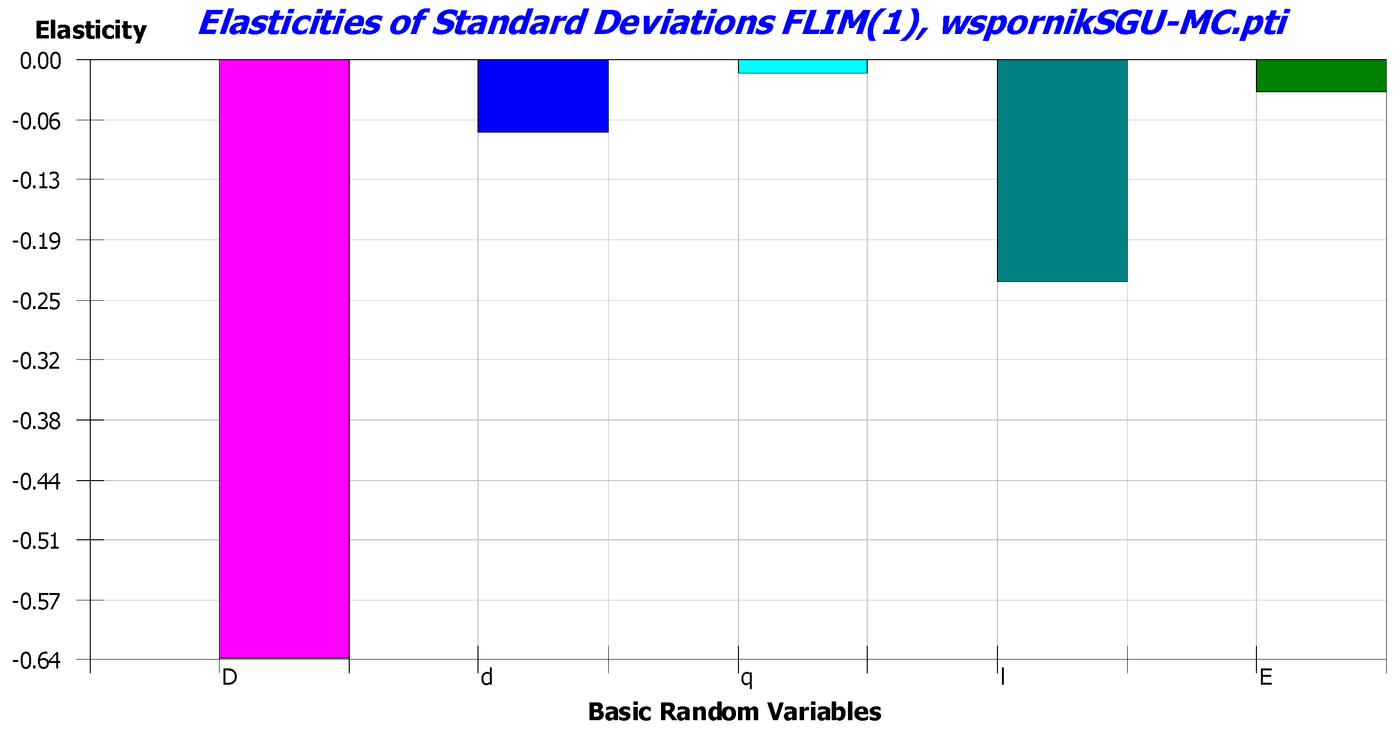
In addition, the coordinates of the vector α and measures of the elasticity of the reliability index due to the mean value and standard deviation were calculated (Figure 6, Figure 7 and Figure 8).
The next step was to calculate the reliability index, failure probability, Bayesian credible interval of failure probability, and first-order Sobol indices using the Monte Carlo method. Below is a description of the results obtained in COMREL.
###################################
Monte Carlo Sampling | Statistics
###################################
Total number of samples: 1,000,000
Total number of failed samples: 52,502
Beta reliability index: 1.621
Estimated probability of failure: 5.3 × 10−2
===================================
Bayesian credible intervals
===================================
upper bound
-----------------------------------
probability that the actual probability of failure does not exceed the indicated value
50%: p_f 5.3 × 10⁻²
75%: p_f 5.3 × 10⁻²
90%: p_f 5.3 × 10⁻²
95%: p_f 5.3 × 10⁻²
99%: p_f 5.3 × 10⁻²
-----------------------------------
equal tail
-----------------------------------
probability that the actual probability of failure is within the specified interval
50%: [5.2 × 10⁻² p_f 5.3 × 10⁻²]
75%: [5.2 × 10⁻² p_f 5.3 × 10⁻²]
90%: [5.2 × 10⁻² p_f 5.3 × 10⁻²
95%: [5.2 × 10⁻² p_f 5.3 × 10⁻²]
99%: [5.2 × 10⁻² p_f 5.3 × 10⁻²]
===================================
Variance based sensitivity analysis
===================================
-----------------------------------
first-order sensitivity index
-----------------------------------
Mean of LSF values: 2.1 × 10⁻¹
Variance of LSF values: 1.5 × 10⁻²
Standard deviation of LSF values: 1.2 × 10⁻¹
C.o.V. of LSF values: 5.7 × 10⁻¹
Variable|S_i
--------------------------
D|6.1 × 10⁻¹
d|6.3 × 10⁻²
q|1.7 × 10⁻²
l|2.7 × 10⁻¹
E|3.8 × 10⁻²
--------------------------
Sum of S_i|1.0 × 100
==========================
The ultimate limit state (ULS) function is defined as the difference between the bending resistance of the beam M d = f y W y = f y D 4 d 4 6 D and the bending moment M = q l 2 2 :
f ULS ( x ) =   M d q l 2 2
As a first step, the reliability index and probability of failure were calculated using the FORM and SORM (Table 3).
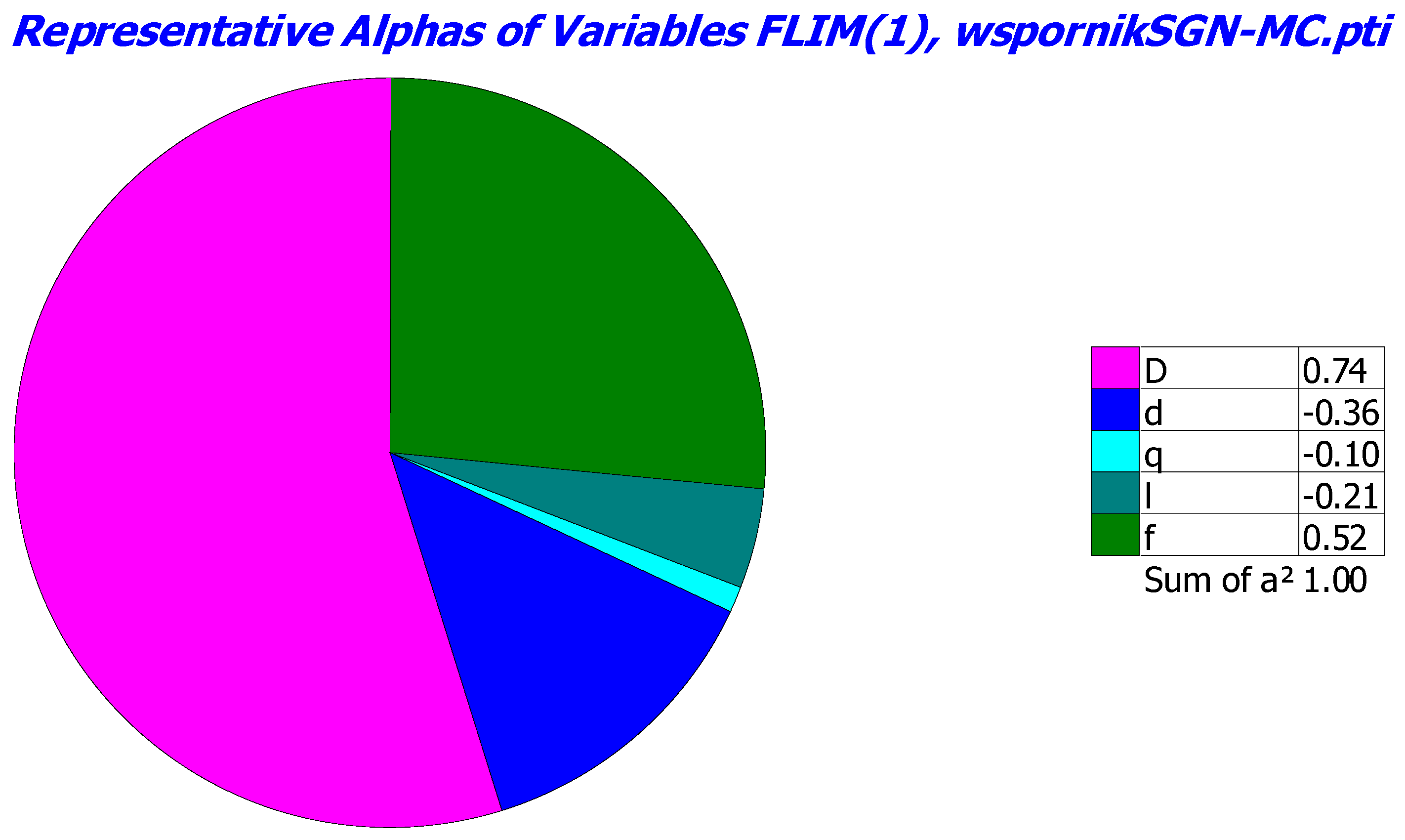
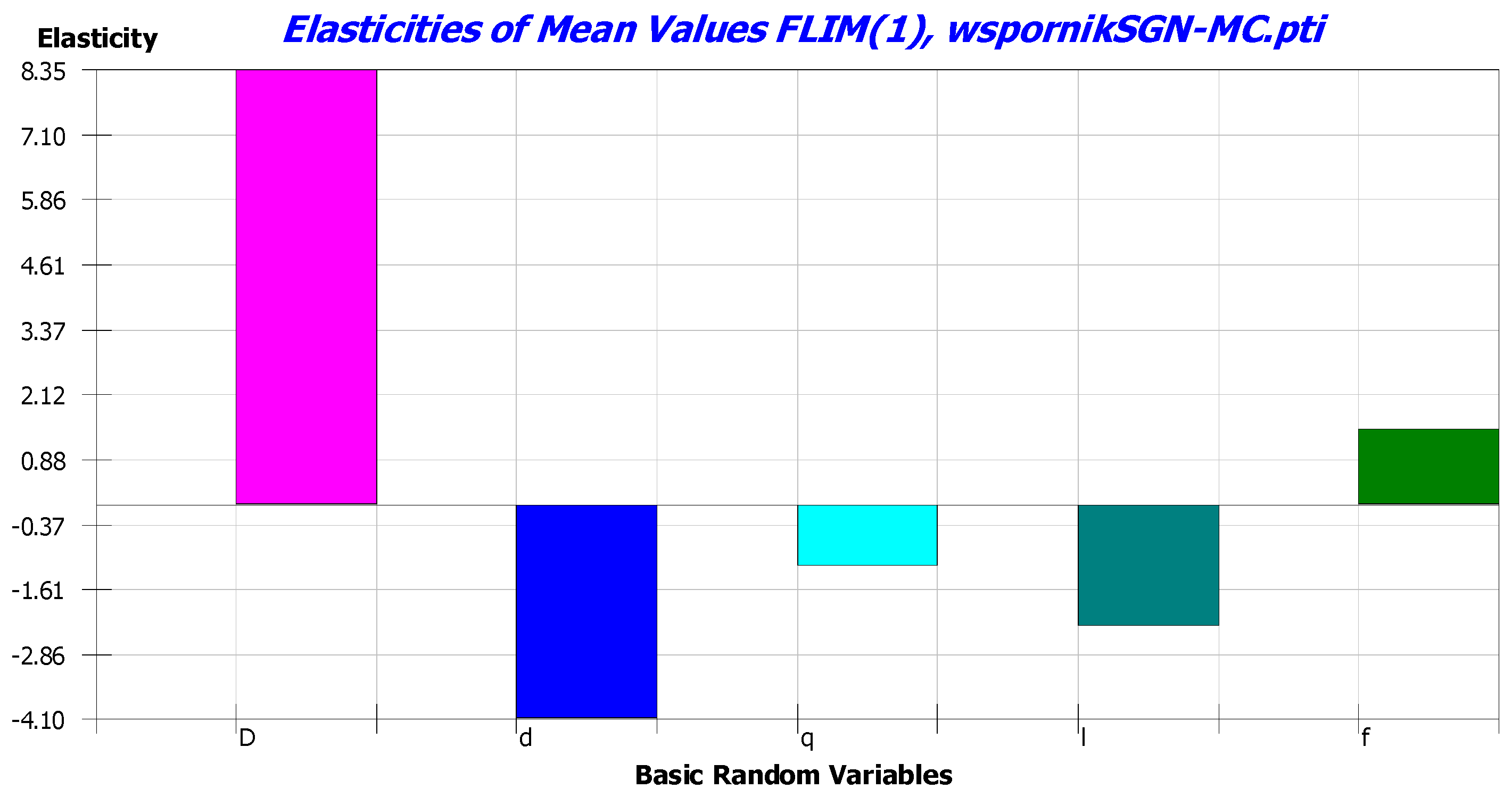
In addition, the coordinates of the vector α and measures of the elasticity of the reliability index due to the mean value and standard deviation for ULS were calculated (Figure 9, Figure 10 and Figure 11).
The next step was to calculate the reliability index, failure probability, Bayesian credible interval of failure probability and first-order Sobol indices using the Monte Carlo method. Below is a description of the results obtained in COMREL.
Monte Carlo Sampling | Statistics
###################################
Total number of samples: 1,000,000
Total number of failed samples: 8
Beta reliability index: 4.388
Estimated probability of failure: 8.0 × 10−6
===================================
Bayesian credible intervals
===================================
upper bound
-----------------------------------
probability that the actual probability of failure does not exceed the indicated value 50%:
p_f 8.7 × 10⁻⁶ 75%:
p_f 1.1 × 10⁻⁵ 90%:
p_f 1.3 × 10⁻⁵ 95%:
p_f 1.4 × 10⁻⁵ 99%:
p_f 1.7 × 10⁻⁵
-----------------------------------
equal tail
-----------------------------------
probability that the actual probability of failure is within the specified interval
50%: [6.8 × 10⁻⁶ p_f 1.1 × 10⁻⁵]
75%: [5.7 × 10⁻⁶ p_f 1.2 × 10⁻⁵]
90%: [4.7 × 10⁻⁶ p_f 1.4 × 10⁻⁵]
95%: [4.1 × 10⁻⁶ p_f 1.6 × 10⁻⁵]
99%: [3.1 × 10⁻⁶ p_f 1.9 × 10⁻⁵]
===================================
Variance based sensitivity analysis
===================================
-----------------------------------
first-order sensitivity index
-----------------------------------
Mean of LSF values: 7.0 × 10²
Variance of LSF values: 3.3 × 10⁴
Standard deviation of LSF values: 1.8 × 10²
C.o.V. of LSF values: 2.6 × 10⁻¹
Variable|S_i
--------------------------
D|5.3 × 10⁻¹
d|7.8 × 10⁻²
q|5.4 × 10⁻³
l|2.2 × 10⁻²
f|3.6 × 10⁻¹
--------------------------
Sum of S_i|1.0 × 100
Values of the Sobol indices and the coordinate vector α | | for SLS and ULS are listed in Table 4.
Comparing the values of vector α obtained using FORM with the values of the Sobol indices from the Monte Carlo method, a consistent trend can be observed.

4. Discussion

Based on the drawings, we observe that in the serviceability limit state, the most significant influence on the probability of failure comes from random variables associated with the beam’s geometry: D, d, l. Negative values associated with the random variables d and l indicate that an increase in these quantities will lead to a decrease in the reliability index, both in terms of mean values and standard deviation. An increase in d will reduce the moment of inertia of the cross-sectional area of the rod, consequently increasing displacement. The length of the rod, l, in the displacement expression is raised to the fourth power in the numerator, hence an increase in this quantity will also result in an increase in displacement. An increase in the dimension D of the cross-sectional area of the rod will increase the moment of inertia, significantly reducing displacement. This quantity, both in the α vector and in the elasticity of reliability index, is positive and has the highest value. The influence of changes in Young’s modulus E and load q on the probability of failure is minimal. In further calculations, these quantities can be treated as deterministic.
The probability of failure associated with the ultimate limit state depends, of course, on changes in the dimensions of the cross-sectional area, D and d. The elasticity of reliability index with respect to the mean value of the random variable D is +7.37, while for the random variable d, it is—4.15. An increase in the mean value of the random variable d will result in a decrease in the reliability index associated with a reduction in the moment of inertia. The influence of changes in the yield strength fy is significant. The influence of changes in the load and length of the beam is significantly smaller.
The authors present two alternative ways of designing in a probabilistic approach using the FORM (SORM) and Monte Carlo simulation. The approximation FORM cannot be used in every case in connection with gradient determination problems. In such cases, it is worth using the Monte Carlo simulation method. The results of both methods are comparable.

5. Conclusions

Every engineering structure must be stable and serviceable throughout its service life. The designer (Engineer) is responsible for designing it in such a way that it meets safety requirements. An alternative method for this approach is given in Annex C of Eurocode 0. The safety of the structure can be assessed probabilistically using reliability techniques. The use of probabilistic techniques in the design usually makes it more complex than the design based on the classical partial safety factor method. There is already software that successfully combines finite element method modules with reliability analysis software. An interesting review of the available software is given in papers [46,47,48,49,50,51,52,53,54,55]. Sensitivity analysis is extremely important in assessing the current condition of the structure as well as in structural health monitoring. The choice of the sensitivity analysis method should be guided by the goals. Following Saltelli [56], possible goals of sensitivity analysis are understanding the robustness of a model with respect to assumptions made on the model input, ranking input factors according to their importance, identifying input factors that are of minor importance and can potentially be omitted, and identifying the areas of the input random variable’s outcome space that lead to extreme model outputs, such as a failure event. From an engineering perspective, the most important goal is decision support. The engineer should understand the effect of changing specific decision variables on the performance of the system. Information obtained from sensitivity analysis enables safe optimization of the design.

Author Contributions

Conceptualization, U.R. and P.Z.; methodology, U.R. and P.Z.; software, U.R. and P.Z.; validation, U.R. and P.Z.; formal analysis U.R. and P.Z.; investigation U.R. and P.Z.; resources U.R. and P.Z.; data curation, U.R. and P.Z.; writing—original draft preparation, U.R. and P.Z.; writing—review and editing, U.R. and P.Z.; visualization, U.R. and P.Z.; supervision, U.R. and P.Z.; project administration, U.R. and P.Z.; funding acquisition, U.R. and P.Z. All authors have read and agreed to the published version of the manuscript.

Funding

This paper was supported by the statutory work no. 02.0.20.00/1.02.001, SUBB. BKTK. 24.001 of the Kielce University of Technology.

Institutional Review Board Statement

Not applicable.

Informed Consent Statement

Not applicable.

Data Availability Statement

The original contributions presented in the study are included in the article, further inquiries can be directed to the corresponding author.

Conflicts of Interest

The authors declare no conflicts of interest.

References

  1. Song, S.; Lu, Z.; Qiao, H. Subset Simulation for Structural Reliability Sensitivity Analysis. Reliab. Eng. Syst. Saf. 2009, 94, 658–665. [Google Scholar] [CrossRef]
  2. Dubourg, V.; Sudert, B. Meta-Model-Based Importance Sampling for Reliability Sensitivity Analysis. Struct. Saf. 2014, 49, 27–36. [Google Scholar] [CrossRef]
  3. Papaioannou, I.; Breitung, K.; Straub, D. Reliability Sensitivity Estimation with Sequential Importance Sampling. Struct. Saf. 2018, 75, 24–34. [Google Scholar] [CrossRef]
  4. Helton, J.C.; Johnson, J.D.; Sallaberry, C.J.; Storlie, C.B. Survey of Sampling-Based Method for Uncertainty and Sensitivity Analysis. Reliab. Eng. Syst. Saf. 2006, 91, 1175–1209. [Google Scholar] [CrossRef]
  5. Chun, M.H.; Han, S.J.; Tak, N.I. An Uncertainty Importance Measure Using a Distance Metric for the Change in a Cumulative Distribution Function. Reliab. Eng. Syst. Saf. 2009, 94, 596–603. [Google Scholar] [CrossRef]
  6. Borgonovo, E. Measuring Uncertainty Importance: Investigation and Comparison of Alternative Approaches. Risk Anal. 2006, 26, 1349–1361. [Google Scholar] [CrossRef] [PubMed]
  7. Li, L.; Lu, Z.; Feng, J.; Wang, B. Moment Independent Importance Measure of Basic Variable and Its State Dependent Parameter Solution. Struct. Saf. 2012, 38, 40–47. [Google Scholar] [CrossRef]
  8. Wang, Q.A.; Liu, Q.A.; Ma, Z.G.; Wang, J.F.; Ni, Y.Q.; Ren, W.X.; Wang, H.B. Data Interpretation and Forecasting of SHM Heteroscedastic Measurements Under Typhoon Conditions Enabled by an Enhanced Hierarchical Sparse Bayesian Learning Model with High Robustness. Measurement 2024, 230, 114509. [Google Scholar] [CrossRef]
  9. Wang, Q.-A.; Dai, Y.; Ma, Z.-G.; Ni, Y.Q.; Tang, J.Q.; Xu, X.Q.; Wu, Z.Y. Towards Probabilistic Data-Driven Damage Detection in SHM Using Sparse Bayesian Learning Scheme. Struct. Control. Health Monit. 2022, 29, e3070. [Google Scholar] [CrossRef]
  10. Zheng, X.-W.; Li, H.-N.; Lv, H.-L.; Huo, L.-S.; Zhang, Y.-Y. Bayesian-Based Seismic Resilience Assessment for High-Rise Buildings with the Uncertainty in Various Variables. J. Build. Eng. 2022, 51, 104321. [Google Scholar] [CrossRef]
  11. Zheng, X.-W.; Li, H.-N.; Shi, Z.-Q. Hybrid AI-Bayesian-Based Demand Models and Fragility Estimates for Tall Buildings Against Multi-Hazard of Earthquakes and Winds. Thin Walled Struct. 2023, 187, 110749. [Google Scholar] [CrossRef]
  12. Zheng, X.-W.; Li, H.-N.; Gardoni, P. Hybrid Bayesian-Copula-Based Risk Assessment for Tall Buildings Subject to Wind Loads Considering Various Uncertainties. Reliab. Eng. Syst. Saf. 2023, 233, 109100. [Google Scholar] [CrossRef]
  13. Sobol, I.M. Global Sensitivity Indices for Nonlinear Mathematical Models and Their Monte Carlo Estimates. Math. Comput. Simul. 2001, 55, 271–280. [Google Scholar] [CrossRef]
  14. Sobol, I.M. Sensitivity Estimates for Nonlinear Mathematical Models. Math. Modell. Comput. Exp. 1993, 1, 407–414. [Google Scholar]
  15. Iman, R.L.; Hora, S.C. A Robust Measure of Uncertainty Importance for Use in Fault Tree System Analysis. Risk Anal. 1990, 10, 401–406. [Google Scholar] [CrossRef]
  16. Szepietowska, K.; Magnain, B.; Lubowiecka, I.; Florentin, E. Sensitivity Analysis Based on Non-Intrusive Regression-Based Polynomial Chaos Expansion for Surgical Mesh Modelling. Struct. Multidisc. Optim 2018, 57, 1391–1409. [Google Scholar] [CrossRef]
  17. Szepietowska, K.; Lubowiecka, I.; Magnain, B.; Florentin, E. Modelling of Abdominal Wall Under Uncertainty of Material Properties. In Computer Methods, Imaging and Visualization in Biomechanics and Biomedical Engineering, Lecture Notes in Computational Vision and Biomechanics, 36, Proceedings of the 16th International Symposium on Computer Methods in Biomechanics and Biomedical Engineering, New York, NY, USA, 14–16 August 2019; Ateshian, G., Myers, K., Tavares, J., Eds.; Springer: Berlin/Heidelberg, Germany, 2020. [Google Scholar]
  18. Ghanem, R.G.; Spanos, P.D. Stochastic Finite Elements: A Spectral Approach; Springer: New York, NY, USA, 1991. [Google Scholar]
  19. Sudret, B. Global Sensitivity Analysis Using Polynomial Chaos Expansions. Reliab. Eng. Syst. Saf. 2008, 93, 964–979. [Google Scholar] [CrossRef]
  20. Crestaux, T.; Le Maître, O.; Martinez, J.M. Polynomial Chaos Expansion for Sensitivity Analysis. Reliab. Eng. Syst. Saf. 2009, 94, 1161–1172. [Google Scholar] [CrossRef]
  21. Wei, P.; Lu, Z.; Hao, W.; Feng, J.; Wang, B. Efficient Sampling Methods for Global Reliability Sensitivity Analysis. Comput. Phys. Commun. 2012, 183, 1728–1743. [Google Scholar] [CrossRef]
  22. Papaioannou, I.; Straub, D. Variance-Based Reliability Sensitivity Analysis and the FORM α-Factors. Reliab. Eng. Syst. Saf. 2021, 210, 107496. [Google Scholar] [CrossRef]
  23. Robert, C.P.; Casella, G. Monte Carlo Statistical Methods; Springer: Berlin/Heidelberg, Germany, 1999. [Google Scholar]
  24. Rubinstein, R.Y.; Kroese, D.P. Simulation and the Monte Carlo Method; Wiley-Interscience: Hoboken, NJ, USA, 2008. [Google Scholar]
  25. Schuëller, G.I. Efficient Monte Carlo Simulation Procedures in Structural Uncertainty and Reliability Analysis—Recent Advances. Struct. Eng. Mech. 2009, 32, 1–20. [Google Scholar] [CrossRef]
  26. Pradlwarter, H.J.; Schuëller, G.I.; Koutsourelakis, P.S.; Charmpis, D.C. Application of Line Sampling Simulation Method to Reliability Benchmark Problems. Struct. Saf. 2007, 29, 208–221. [Google Scholar] [CrossRef]
  27. Papaioannou, I.; Straub, D. Combination Line Sampling for Structural Reliability Analysis. Struct. Saf. 2021, 88, 102025. [Google Scholar] [CrossRef]
  28. Papaioannou, I.; Papadimitriou, C.; Straub, D. Sequential Importance Sampling for Structural Reliability Analysis. Struct. Saf. 2016, 62, 66–75. [Google Scholar] [CrossRef]
  29. Rackwitz, R.; Flessler, B. Structural Reliability Under Combined Random Load Sequences. Comput. Struct. 1978, 9, 489–494. [Google Scholar] [CrossRef]
  30. Hasofer, A.M.; Lind, N.C. Exact and Invariant Second Moment Code Format. J. Eng. Mech. Div. ASCE 1974, 100, 111–121. [Google Scholar] [CrossRef]
  31. Hohenbichler, M.; Gollwitzer, S.; Kruse, W.; Rackwitz, R. New Light on First and Second Order Reliability Thods. Struct. Saf. 1987, 4, 267–284. [Google Scholar] [CrossRef]
  32. Breitung, K.; Hohenbichler, M. Asymptotic Approximations for Multivariate Integrals with an Application to Multinormal Probabilities. J. Multivar. Anal. 1989, 30, 80–97. [Google Scholar] [CrossRef]
  33. Fiessler, B.; Neumann, H.-J.; Rackwitz, R. Quadratic Limit States in Structural Reliability. J. Eng. Mech. Div. ASCE 1979, 105, 661–676. [Google Scholar] [CrossRef]
  34. Abdo, T.; Rackwitz, R. Reliability of Uncertain Structural Systems. Proc. Finite Elem. Eng. Appl. 1990, 805, 161–176. [Google Scholar]
  35. Schittkowski, K. The Nonlinear Programming Method of Wilson, Han and Powell with an Augmented Lagrangian Type Line Search Function, Part 1: Convergence Analysis. Numer. Math. 1982, 38, 83–114. [Google Scholar] [CrossRef]
  36. Schittkowski, K. User’s Guide for the Nonlinear Programming Code NLPQL, Handbook to Optimization Program Package NLPQL; University of Stuttgart: Stuttgart, Germany, 1985. [Google Scholar]
  37. Schittkowski, K.; Zillober, C.; Zotemantel, R. Numerical Comparison of Nonlinear Programming Algorithms for Structural Optimization. Struct. Multidiscip. Optim. 1994, 7, 1–19. [Google Scholar] [CrossRef]
  38. Arora, J.S. Introduction to Optimum Design; McGraw-Hill: New York, NY, USA, 1989. [Google Scholar]
  39. Zabojszcza, P.; Radoń, U. Optimization of Steel Roof Framing Taking into Account the Random Nature of Design Parameters. Materials 2022, 15, 5017. [Google Scholar] [CrossRef]
  40. Zabojszcza, P.; Radoń, U. Stability Analysis of the Single-Layer Dome in Probabilistic Description by the Monte Carlo Method. J. Theor. Appl. Mech. 2020, 58, 425–436. [Google Scholar] [CrossRef]
  41. Hohenbichler, M.; Rackwitz, R. Improvement of Second-Order Reliability Estimates by Importance Sampling. J. Eng. Mech. ASCE 1988, 114, 2195–2199. [Google Scholar] [CrossRef]
  42. Doliński, K. Importance Sampling Techniques in Reliability Calculations; IPPT: Warsaw, Poland, 1988; Volume 37. [Google Scholar]
  43. Fujita, M.; Rackwitz, R. Updating First and Second Order Reliability Estimates by Importance Sampling. Proc. Jpn. Soc. Civ. Eng. 1988, 392, 53–59. [Google Scholar] [CrossRef]
  44. de Angelis, M.; Patelli, E.; Beer, M. Advanced Line Sampling for Efficient Robust Reliability Analysis. Struct. Saf. 2015, 52, 170–182. [Google Scholar] [CrossRef]
  45. Bucher, C.G. Adaptive Sampling—An Iterative Fast Monte Carlo Procedure. Struct. Saf. 1988, 5, 119–126. [Google Scholar] [CrossRef]
  46. Schuëller, G.I.; Pradlwarter, H.J. Computational Stochastic Structural Analysis (COSSAN)—Software Tool. Struct. Saf. 2006, 28, 68–82. [Google Scholar] [CrossRef]
  47. Reh, S.; Beley, J.D.; Mukherjee, S.; Khor, E.H. Probabilistic Finite Element Analysis Using ANSYS. Struct. Saf. 2006, 28, 17–43. [Google Scholar] [CrossRef]
  48. Pellissetti, M.F.; Schuëller, G.I. On General Purpose Software in Structural Reliability—An Overview. Struct. Saf. 2006, 28, 3–16. [Google Scholar] [CrossRef]
  49. Lemaire, M.; Pendola, M. Phimeca-Soft. Struct. Saf. 2006, 28, 130–149. [Google Scholar] [CrossRef]
  50. Lin, H.Z.; Khalessi, M.R. General Outlook of UNIPASSV5.0: A General-Purpose Probabilistic Software System. Struct. Saf. 2006, 28, 196–216. [Google Scholar] [CrossRef]
  51. Gollwitzer, S.; Kirchgabner, B.; Fischer, R.; Rackwitz, R. PERMAS-RA/STRUREL System of Programs for Probabilistic Reliability Analysis. Struct. Saf. 2006, 28, 108–129. [Google Scholar] [CrossRef]
  52. Der Kiureghian, A.; Haukaas, T.; Fujimura, K. Structural Reliability Software at the University of California, Berkeley. Struct. Saf. 2006, 28, 44–67. [Google Scholar] [CrossRef]
  53. Thacker, B.H.; Riha, D.S.; Fitch, S.K.H.; Huyse, L.J.; Pleming, J.B. Probabilistic Engineering Analysis Using the NESSUS Software. Struct. Saf. 2006, 28, 83–107. [Google Scholar] [CrossRef]
  54. Tvedt, L. Proban-Probabilistic Analysis. Struct. Saf. 2006, 28, 150–163. [Google Scholar] [CrossRef]
  55. Wu, Y.T.; Shin, Y.; Sues, R.H.; Cesare, M.A. Probabilistic Function Evaluation System (ProFES) for Reliability-Based Design. Struct. Saf. 2006, 28, 164–195. [Google Scholar] [CrossRef]
  56. Saltelli, A.; Ratto, M.; Andres, T.; Campolongo, F.; Cariboni, J.; Gatelli, D.; Saisana, M.; Tarantola, S. Global Sensitivity Analysis. The Primer; John Wiley & Sons: Hoboken, NJ, USA, 2008. [Google Scholar]
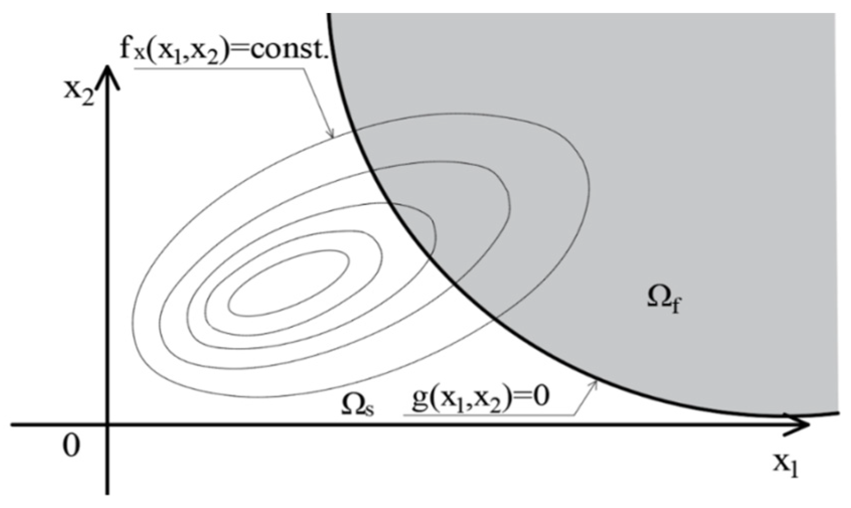
Figure 1. Illustration of limit state function g(x), safe area Ωs, and failure area Ωf for two random variables.
Applsci 15 00342 g001
Figure 2. Transformation of a limit state function to a standard Gaussian space.
Applsci 15 00342 g002
Figure 3. Concept of the Monte Carlo method.
Applsci 15 00342 g003
Figure 4. Illustration of the elasticity of reliability index β as a function of parameter p.
Applsci 15 00342 g004
Figure 5. Geometry and load of the cantilever beam.
Applsci 15 00342 g005
Figure 6. Graphical illustration of the coordinates of vector α for SLS.
Applsci 15 00342 g006
Figure 7. Graphical illustration of the elasticity of the reliability index based on mean value for SLS.
Applsci 15 00342 g007
Figure 8. Graphical illustration of the elasticity of the reliability index based on standard deviation for SLS.
Applsci 15 00342 g008
Figure 9. Graphical illustration of the coordinates of vector α for ULS.
Applsci 15 00342 g009
Figure 10. Graphical illustration of the elasticity of the reliability index based on mean value for ULS.
Applsci 15 00342 g010
Figure 11. Graphical illustration of the elasticity of the reliability index based on standard deviation for ULS.
Applsci 15 00342 g011
Table 1. Description of random variables.
Random VariableMean ValueStandard DeviationCoefficient of Variation
D8 cm0.16 cm2%
d6 cm0.12 cm2%
E21,000 kN/cm2630 kN/cm23%
q0.06 kN/cm0.0012 kN/cm2%
l150 cm3 cm2%
fy23.5 kN/cm21.88 kN/cm28%
Table 2. Estimation of reliability index and failure probability for serviceability limit state function.
FORMSORM
reliability index1.6341.62
failure probability5.11 × 10−25.26 × 10⁻²
Table 3. Estimation of reliability index and failure probability for ultimate limit state function.
FORMSORM
reliability index4.4344.388
failure probability4.62 × 10−65.73 × 10⁻⁶
Table 4. The values of Sobol indices and coordinate α vector | | for SLS and ULS.
VariableSLSULS
Sobol Index SiCoordinate α Vector | |Sobol Index SiCoordinate α Vector | |
D6.1 × 10−18.0 × 10−15.3 × 10−17.9 × 10⁻¹
l2.7 × 10−14.9 × 10−12.2 × 10−22.1 × 10⁻¹
d6.3 × 10−22.8 × 10−17.8 × 10−23.6 × 10⁻¹
E3.8 × 10−21.9 × 10⁻¹--
fy--3.6 × 10−15.2 × 10−1
q1.7 × 10−21.2 × 10−15.4 × 10−31.0 × 10⁻¹
Disclaimer/Publisher’s Note: The statements, opinions and data contained in all publications are solely those of the individual author(s) and contributor(s) and not of MDPI and/or the editor(s). MDPI and/or the editor(s) disclaim responsibility for any injury to people or property resulting from any ideas, methods, instructions or products referred to in the content.