
STGAN: Swin Transformer-Based GAN to Achieve Remote Sensing Image Super-Resolution Reconstruction


Abstract
1. Introduction
- We have innovatively designed a remote sensing image RefSR method (STGAN) based on the Generative Adversarial Networks (GANs) and self attention mechanism. STGAN adopts the GAN structure and introduces a specific improved Swin Transformer model. At the same time, it combines the residual network, the self-attention mechanism, and the dual-channel feature extraction of CNN to achieve accurate pixel-level fusion and significantly improve the quality of image reconstruction.
- The experimental results verify the excellent performance of STGAN in the field of super-resolution, which not only excels in many SISR solutions, but also demonstrates obvious advantages in comparison with mainstream RefSR methods. The STGAN is robust to the fluctuation of reference image quality and extends the upper performance limit of the SR task to a certain extent, which fully proves the RefSR method’s great potential of RefSR methods in the field of remote sensing.Our experimental data can be found on https://github.com/hw-star/STGAN, accessed on 27 December 2024.
2. Related Work
2.1. SR for Remote Sensing Images
2.2. Swin Transformer
2.3. RefSR
3. Method
3.1. Overview
3.2. Network Architecture
3.2.1. Generator
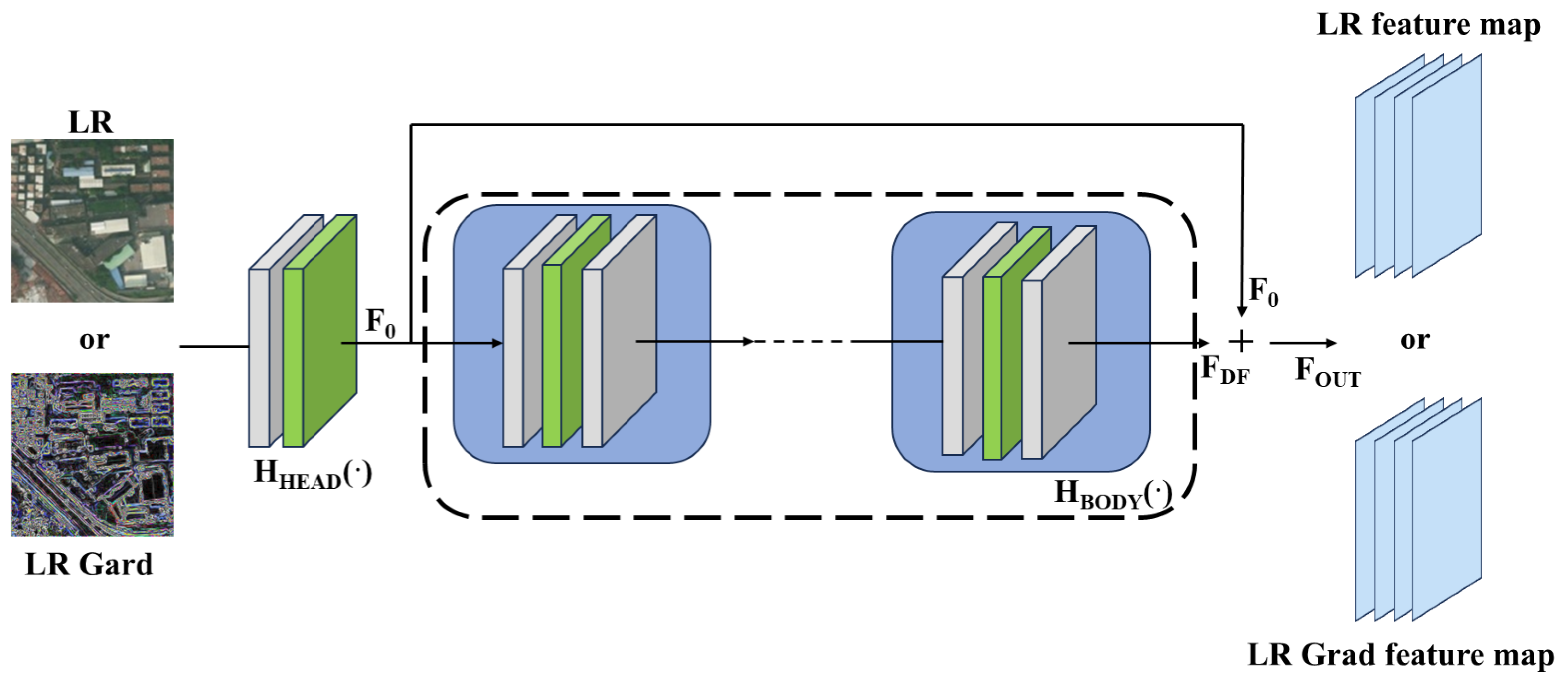
- Feature extraction module (SFE):Given a low-quality (LR) input (where H, W, and C are the image height, width, and the number of input channels, respectively), as shown in Figure 3, a convolutional layer (using a 3 × 3 convolutional kernel as well as a Leaky ReLU activation function) is firstly utilized to extract the shallow feature as: , and secondly, the deep feature as:where consists of multiple residual blocks (ResBlocks). Each residual block contains two convolutional layers inside, both of which use a 3 × 3 convolutional kernel and the same number of filters to ensure that the dimensionality of the input and output is consistent. It has been shown [44,45] that deep convolutional networks help to improve super-resolution performance. Finally, the shallow feature and the deep feature are summed up by residual concatenation to obtain the final output feature: . The design of the residual block is crucial when training deep networks, as it effectively mitigates the problems of gradient vanishing and gradient explosion, ensuring that information can be effectively passed through the network. In addition, the role of the SFE module is to perform shallow feature processing, and it is capable of performing image feature extraction and gradient map feature processing independently, respectively.
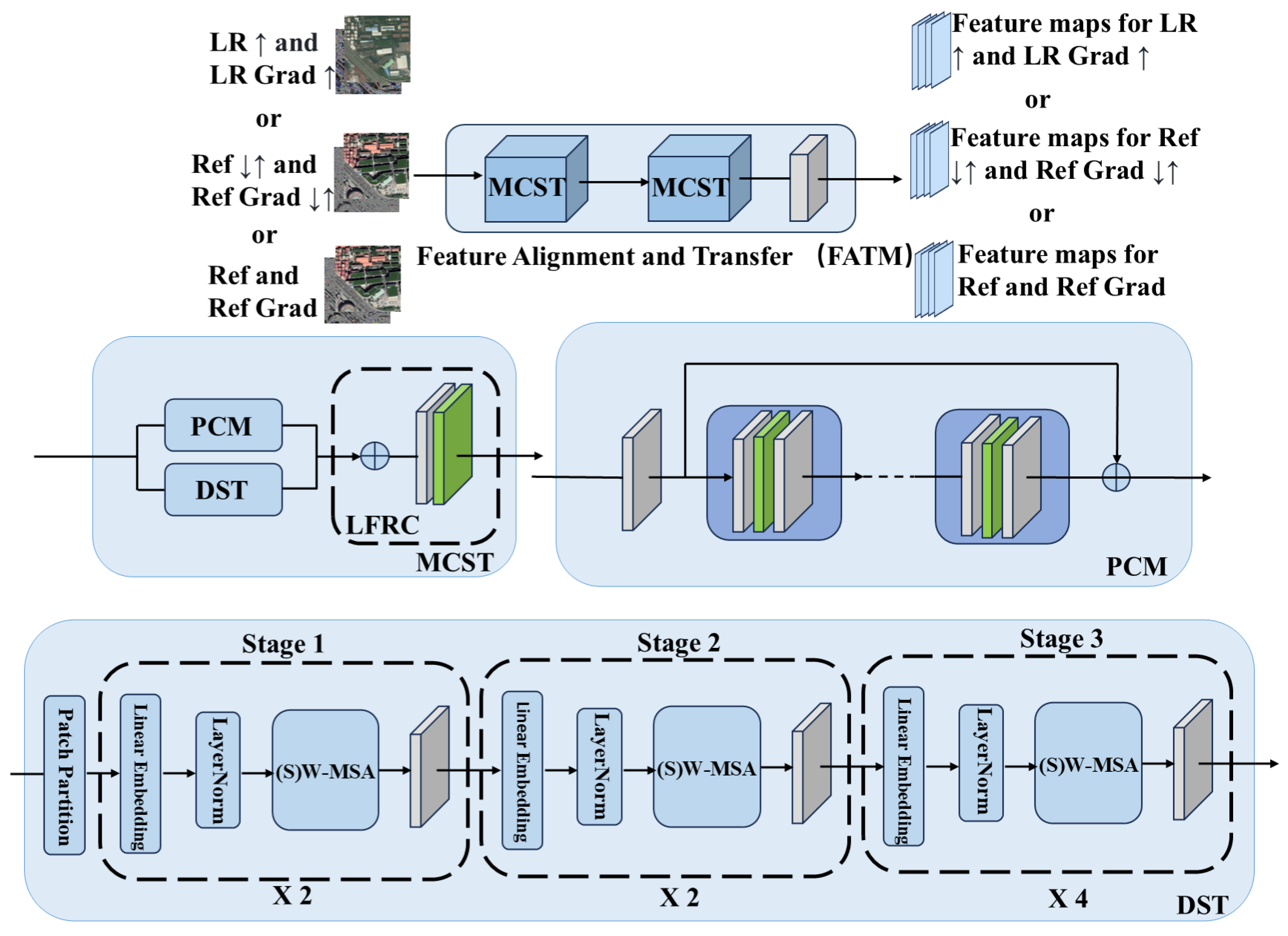
- Feature alignment and transfer module:In this module, as shown in Figure 4, two CNN-Swin Transformer blocks (MCST) and a fusion convolution block (LFRC) are included. Each MCST block adopts a two-channel design based on CNN and a specific modification of Swin Transformer, respectively. The Patch Convolutional Module (PCM) is adapted with a feature extraction module specifically designed for extracting rich features from the input image as:where consists of multiple residual blocks. PCM is responsible for local feature extraction, capturing basic features such as edges and texture of the image through a series of residual convolutional layers. The input image is first passed through an initial convolutional layer to extract primary features, and then further processed through multiple ResBlocks to capture more complex features. To maintain training stability and facilitate feature transfer, PCM employs residual connections in each ResBlock. Finally, the shallow and deep features integrated through residual concatenation from the final output . Deepened Swin Transformer (DST) is an adaptation of the Swin Transformer architecture based on the 7 × 7 sliding window mechanism, and is specifically designed to capture global detailed features of an image. The module keeps the (S)W-MSA mechanism of Swin Transformer unchanged while adding a convolutional layer at the end of it to further enhance the local feature extraction capability. In addition, DST fixes the size of the feature maps at each stage to improve the stability and consistency of feature extraction while maintaining the global context modeling capability. In this design, PCM and DST extract local and global features independently. To enhance the representational capability of the model, LFRC performs channel-level fusion of the features extracted by PCM and DST to generate a rich feature representation that integrates both global and local information.In the RefSR method, the module is designed to process multiple input data streams, including low-resolution (LR) images, reference (Ref) images, and their corresponding gradient maps, separately. Processing a set of corresponding images and gradient maps at a time allows the module to simultaneously analyze and integrate information from different sources, thus significantly improving the quality of the super-resolution reconstruction. By fusing local and global information, the module not only enhances the overall performance of the image, but also uses the gradient information to further optimize the edge and texture details, resulting in more accurate feature alignment and generating more natural and realistic visual effects.
- High-quality remote sensing image reconstruction moduleInstead of simply merging various image features as well as gradient feature map features, we employ a fine-grained feature fusion strategy. Our goal is to enhance the correlation between the two features while suppressing the less correlated information to optimize the texture transfer process. As shown in Figure 5, the first and second set of features are first fused at the channel layer, and then attention maps are generated through a series of convolutional layers. These attention maps are normalized by a sigmoid function and elementwise multiplied with the second set of features to strengthen the correlation between them. Next, the attention maps are again convolved and the results are summed with the previous results to further enrich the features. Finally, the enriched features are fused with the first set of features at the channel level to provide more accurate and enriched information for the subsequent texture transfer process. The Robustness Augmentation Module (RAM-V) is employed, the equation of which can be expressed as:where denotes the summed enriched features, and denote the first set of features and the second set of features, respectively, and and denote the computation including convolutional layers.
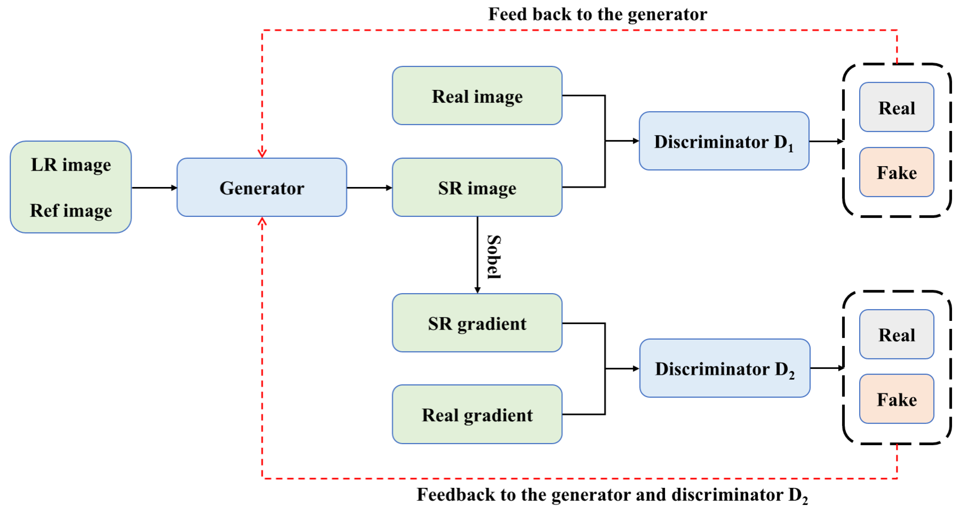
3.2.2. Discriminators
3.3. Loss Function
- Reconstruction Loss: It is used to measure the similarity between the reconstructed image and the high-resolution image to ensure that the reconstructed image is close to the target high-resolution image at the pixel level. The reconstruction loss is defined as:where denotes the HR image, denotes the SR image, = G(), G(·) denotes the generator, and denotes the LR image.
- Adversarial Loss: The discriminator in the generative adversarial network is used to generate more realistic images, and the generative ability of the model is enhanced by adversarial training. The optimization between generator G and discriminator is as follows:where aims to distinguish between the real and generated .
- Perceptual Loss: By mimicking the properties of the human visual system, a pre-trained network is used to measure the difference in perceptual space between the reconstructed image and the high-resolution image. The perceptual loss is defined as:where denotes the layer i output of ResNet-50.
- Gradient Loss: It is a key component used to maintain the image geometry in super-resolution tasks and ensures the sharpness of image edges and structures by limiting the second-order relationship between neighboring pixels. In the computation process, the gradient loss is obtained by comparing the gradient of a super-resolution image () with that of a high-resolution image (), i.e., by solving for the difference between neighboring pixels. This includes the gradient reconstruction loss () and the gradient adversarial loss (), defined as:where M(·) denotes the gradient operation and aims to distinguish between the real M () and generated M ().
3.4. Implementation Details
4. Experiments
4.1. Datasets
4.2. Assessment of Indicators
- PSNR measures the image quality by calculating the mean square error (MSE) between the original image and the processed image, and its value is measured in decibels (dB), which reflects the pixel-level difference of the image, and usually, a higher PSNR value indicates a better-quality image. The PSNR is calculated as:where N is the total number of pixels in the image, are the values of the original and reconstructed images at the ith pixel, respectively, R is the maximum possible pixel value (for 8-bit images, R = 255), and MSE is the mean square error.
- SSIM further takes into account the brightness, contrast, and structural information of an image and evaluates the similarity of two images by comparing their differences in these aspects, with a value between 0 and 1, with the closer to 1 indicating the better quality of the image. The formula for calculating SSIM is:where and are the mean values of the images x and y, and are their variances, is their covariance, and and are small constants introduced to avoid a zero denominator.
- PI and Natural Image Quality Evaluator (NIQE) [57] can be used as metrics for the evaluation of real images. NIQE and PI were originally introduced as nonreference image quality assessment methods based on low-level statistical features [58]. NIQE is obtained by computing 36 identical Natural Scene Statistical (NSS) features from the same-sized patches in an image. PI is calculated by merging the criteria of Ma et al. and NIQE [59] as follows:
- LPIPS is a full reference metric that measures perceptual image similarity using a pre-trained deep network. We use the AlexNet [60] model to compute the distance in feature space. LPIPS can be computed using a given image y and the real image as follows:where and denote the height and width of layer lth, respectively, and denote the features corresponding to y and of layer lth at position (h, w), respectively, is the learned weight vector, and ⊙ is the elementwise multiplication operation.
- SAM is mainly used to measure the consistency between the reconstructed image and the original image in terms of spectral information, which calculates the angle between the spectral vectors of the reconstructed image and the corresponding pixels of the real image; the smaller the angle is, the more similar the spectral distributions of the two are, and the better the spectral information is retained. The formula is as follows:where M is the dimension (i.e., number of bands) of each spectral vector, and denote the value of the jth band at the ith pixel for image 1 and image 2, respectively, and N is the total number of pixels in the image.
- RMSE calculates the pixel error between the reconstructed image and the original high-resolution image; the smaller the value, the closer the reconstructed image is to the real image and the smaller the error. The formula is as follows:where N is the total number of data points, is the actual observed value, and is the model predicted value.
4.3. Quantitative and Qualitative Comparison of Different Methods
4.4. Ablation Experiments
- Analysis of the effectiveness of the RefSR:To validate the effectiveness of the RefSR method, we conducted comparison experiments, keeping the same training strategy and network parameters. In the comparison experiments, the baseline method is constructed using only a convolutional neural network without the self-attention mechanism, while the STGAN(SISR) model removes all the reference image inputs and simulates the traditional SISR method by using only the LR images and their corresponding gradient maps for super-resolution reconstruction. The experimental results, as shown in Table 3, show that the RefSR method significantly improves the performance of super-resolution reconstruction through the synergistic effect of multiple image inputs and outperforms the SISR method and the baseline method. In addition, the gradual introduction of more depth-referenced features further enhances the reconstruction effect. Based on this, our method employs three levels of reference features to maximize the utilization of multi-image information, thus achieving better super-resolution reconstruction performance.
- Effectiveness of RAM-V:In order to verify the effectiveness of RAM-V, we removed RAM-V in the feature transfer process and replaced it with direct channel-level fusion of the inputs and processed them through a convolutional neural network instead. As shown in Table 4, the use of RAM-V significantly improves the robustness of the model in different scenarios. This is because RAM-V is able to suppress the influence of irrelevant information in Ref features and focuses on the relevant regions between LR images and Ref images. Thus, RAM-V significantly improves the robustness of the model by suppressing irrelevant information and enhancing the correlation between the two.
- Effectiveness of gradient loss:We analyze the impact of gradient loss. “Baseline” refers to the use of only common SR loss functions, including reconstruction loss , adversarial loss , and perceptual loss . We added gradient-based reconstruction loss and gradient-based adversarial loss in turn. As shown in Table 5, the gradient loss significantly improves the PI and LPIPS compared to the baseline model, suggesting that it produces more realistic visuals.
- Hyperparameter Tuning of Loss Weight:In our experiments, we used the same training strategy and network parameters, only adjusting the values of ///. As shown in Table 6, the model using the parameter combination /// = 0.1/0.001/1/0.001 performs well on several key metrics. On PSNR and SSIM metrics, the parameter combination achieves the best results on different test sets several times, indicating that the model is able to effectively improve the quality of image reconstruction and maintain structural consistency. Meanwhile, the excellent performance on the LPIPS metric further validates the model’s advantage in perceptual quality. These results indicate that the parameter combination has good robustness and wide adaptability, and is capable of achieving high-quality image super-resolution reconstruction in a variety of scenarios.
5. Conclusions
Author Contributions
Funding
Institutional Review Board Statement
Informed Consent Statement
Data Availability Statement
Acknowledgments
Conflicts of Interest
References
- Chaminé, H.I.; Pereira, A.J.; Teodoro, A.C.; Teixeira, J. Remote sensing and GIS applications in earth and environmental systems sciences. SN Appl. Sci. 2021, 3, 870. [Google Scholar] [CrossRef]
- Pan, B.; Shi, Z.; Xu, X.; Shi, T.; Zhang, N.; Zhu, X. CoinNet: Copy initialization network for multispectral imagery semantic segmentation. IEEE Geosci. Remote Sens. Lett. 2018, 16, 816–820. [Google Scholar] [CrossRef]
- Mathieu, R.; Freeman, C.; Aryal, J. Mapping private gardens in urban areas using object-oriented techniques and very high-resolution satellite imagery. Landsc. Urban Plan. 2007, 81, 179–192. [Google Scholar] [CrossRef]
- Li, W.; He, C.; Fang, J.; Zheng, J.; Fu, H.; Yu, L. Semantic segmentation-based building footprint extraction using very high-resolution satellite images and multi-source GIS data. Remote Sens. 2019, 11, 403. [Google Scholar] [CrossRef]
- Yuan, S.; Dong, R.; Zheng, J.; Wu, W.; Zhang, L.; Li, W.; Fu, H. Long time-series analysis of urban development based on effective building extraction. In Proceedings of the Geospatial Informatics X; SPIE: Bellingham, WA, USA, 2020; Volume 11398, pp. 192–199. [Google Scholar]
- Yang, W.; Zhang, X.; Tian, Y.; Wang, W.; Xue, J.H.; Liao, Q. Deep learning for single image super-resolution: A brief review. IEEE Trans. Multimed. 2019, 21, 3106–3121. [Google Scholar] [CrossRef]
- Kim, J.; Lee, J.K.; Lee, K.M. Accurate image super-resolution using very deep convolutional networks. In Proceedings of the IEEE Conference on Computer Vision and Pattern Recognition, Las Vegas, NV, USA, 27–30 June 2016; pp. 1646–1654. [Google Scholar]
- Lim, B.; Son, S.; Kim, H.; Nah, S.; Mu Lee, K. Enhanced deep residual networks for single image super-resolution. In Proceedings of the IEEE Conference on Computer Vision and Pattern Recognition Workshops, Honolulu, HI, USA, 21–26 July 2017; pp. 136–144. [Google Scholar]
- Yu, J.; Fan, Y.; Yang, J.; Xu, N.; Wang, Z.; Wang, X.; Huang, T. Wide activation for efficient and accurate image super-resolution. arXiv 2018, arXiv:1808.08718. [Google Scholar]
- Wang, P.; Bayram, B.; Sertel, E. A comprehensive review on deep learning based remote sensing image super-resolution methods. Earth-Sci. Rev. 2022, 232, 104110. [Google Scholar] [CrossRef]
- Yue, L.; Shen, H.; Li, J.; Yuan, Q.; Zhang, H.; Zhang, L. Image super-resolution: The techniques, applications, and future. Signal Process. 2016, 128, 389–408. [Google Scholar] [CrossRef]
- Ledig, C.; Theis, L.; Huszar, F.; Caballero, J.; Cunningham, A.; Aitken, A.; Tejani, A.; Wang, Z.; Shi, W. Photo-realistic single image super-resolution using a generative adversarial network. In Proceedings of the IEEE Conference on Computer Vision and Pattern Recognition, Honolulu, HI, USA, 21–26 July 2017; Volume 2017, pp. 4681–4690. [Google Scholar]
- Wang, X.; Yu, K.; Wu, S.; Gu, J.; Liu, Y.; Dong, C.; Qiao, Y.; Change Loy, C. Esrgan: Enhanced super-resolution generative adversarial networks. In Proceedings of the European Conference on Computer Vision (ECCV) Workshops, Munich, Germany, 8–14 September 2018. [Google Scholar]
- Ma, C.; Rao, Y.; Cheng, Y.; Chen, C.; Lu, J.; Zhou, J. Structure-preserving super resolution with gradient guidance. In Proceedings of the IEEE/CVF Conference on Computer Vision and Pattern Recognition, Seattle, WA, USA, 13–19 June 2020; pp. 7769–7778. [Google Scholar]
- Liu, Z.S.; Siu, W.C.; Chan, Y.L. Reference based face super-resolution. IEEE Access 2019, 7, 129112–129126. [Google Scholar] [CrossRef]
- Zheng, H.; Ji, M.; Wang, H.; Liu, Y.; Fang, L. Crossnet: An end-to-end reference-based super resolution network using cross-scale warping. In Proceedings of the European Conference on Computer Vision (ECCV), Munich, Germany, 8–14 September 2018; pp. 88–104. [Google Scholar]
- Zhang, Z.; Wang, Z.; Lin, Z.; Qi, H. Image super-resolution by neural texture transfer. In Proceedings of the IEEE/CVF Conference on Computer Vision and Pattern Recognition, Long Beach, CA, USA, 15–20 June 2019; pp. 7982–7991. [Google Scholar]
- Zhang, L.; Li, X.; He, D.; Li, F.; Wang, Y.; Zhang, Z. Rrsr: Reciprocal reference-based image super-resolution with progressive feature alignment and selection. In Proceedings of the European Conference on Computer Vision, Tel Aviv, Israel, 23–27 October 2022; Springer: Berlin/Heidelberg, Germany, 2022; pp. 648–664. [Google Scholar]
- Dong, C.; Loy, C.C.; He, K.; Tang, X. Learning a deep convolutional network for image super-resolution. In Proceedings of the Computer Vision–ECCV 2014: 13th European Conference, Zurich, Switzerland, 6–12 September 2014; Proceedings, Part IV 13; Springer: Berlin/Heidelberg, Germany, 2014; pp. 184–199. [Google Scholar]
- Shi, W.; Caballero, J.; Huszár, F.; Totz, J.; Aitken, A.P.; Bishop, R.; Rueckert, D.; Wang, Z. Real-time single image and video super-resolution using an efficient subpixel convolutional neural network. In Proceedings of the IEEE Conference on Computer Vision and Pattern Recognition, Las Vegas, NV, USA, 27–30 June 2016; pp. 1874–1883. [Google Scholar]
- Pan, Z.; Ma, W.; Guo, J.; Lei, B. Super-resolution of single remote sensing image based on residual dense backprojection networks. IEEE Trans. Geosci. Remote Sens. 2019, 57, 7918–7933. [Google Scholar] [CrossRef]
- Dong, C.; Loy, C.C.; He, K.; Tang, X. Image super-resolution using deep convolutional networks. IEEE Trans. Pattern Anal. Mach. Intell. 2015, 38, 295–307. [Google Scholar] [CrossRef] [PubMed]
- Kim, J.; Lee, J.K.; Lee, K.M. Deeply-recursive convolutional network for image super-resolution. In Proceedings of the IEEE Conference on Computer Vision and Pattern Recognition, Las Vegas, NV, USA, 27–30 June 2016; pp. 1637–1645. [Google Scholar]
- Jiang, K.; Wang, Z.; Yi, P.; Wang, G.; Lu, T.; Jiang, J. Edge-enhanced GAN for remote sensing image superresolution. IEEE Trans. Geosci. Remote Sens. 2019, 57, 5799–5812. [Google Scholar] [CrossRef]
- Guo, M.; Xiong, F.; Zhao, B.; Huang, Y.; Xie, Z.; Wu, L.; Chen, X.; Zhang, J. TDEGAN: A Texture-Detail-Enhanced Dense Generative Adversarial Network for Remote Sensing Image Super-Resolution. Remote Sens. 2024, 16, 2312. [Google Scholar] [CrossRef]
- Liang, J.; Cao, J.; Sun, G.; Zhang, K.; Van Gool, L.; Timofte, R. Swinir: Image restoration using swin transformer. In Proceedings of the IEEE/CVF International Conference on Computer Vision, Montreal, BC, Canada, 11–17 October 2021; pp. 1833–1844. [Google Scholar]
- Wang, Y.; Liu, Y.; Zhao, S.; Li, J.; Zhang, L. CAMixerSR: Only Details Need More “Attention”. In Proceedings of the IEEE/CVF Conference on Computer Vision and Pattern Recognition, Seattle, WA, USA, 16–22 June 2024; pp. 25837–25846. [Google Scholar]
- Chen, X.; Wang, X.; Zhou, J.; Qiao, Y.; Dong, C. Activating more pixels in image super-resolution transformer. In Proceedings of the IEEE/CVF Conference on Computer Vision and Pattern Recognition, Vancouver, BC, Canada, 17–24 June 2023; pp. 22367–22377. [Google Scholar]
- Vaswani, A. Attention is all you need. In Proceedings of the Advances in Neural Information Processing Systems s (NIPS 2017), Long Beach, CA, USA, 4–9 December 2017. [Google Scholar]
- Mikolov, T. Efficient estimation of word representations in vector space. arXiv 2013, arXiv:1301.3781. [Google Scholar]
- Sutskever, I. Sequence to Sequence Learning with Neural Networks. arXiv 2014, arXiv:1409.3215. [Google Scholar]
- Sarzynska-Wawer, J.; Wawer, A.; Pawlak, A.; Szymanowska, J.; Stefaniak, I.; Jarkiewicz, M.; Okruszek, L. Detecting formal thought disorder by deep contextualized word representations. Psychiatry Res. 2021, 304, 114135. [Google Scholar] [CrossRef] [PubMed]
- Casini, L.; Marchetti, N.; Montanucci, A.; Orrù, V.; Roccetti, M. A human–AI collaboration workflow for archaeological sites detection. Sci. Rep. 2023, 13, 8699. [Google Scholar] [CrossRef]
- Cao, J.; Liang, J.; Zhang, K.; Li, Y.; Zhang, Y.; Wang, W.; Gool, L.V. Reference-based image super-resolution with deformable attention transformer. In Proceedings of the European Conference on Computer Vision, Tel Aviv, Israel, 23–27 October 2022; Springer: Berlin/Heidelberg, Germany, 2022; pp. 325–342. [Google Scholar]
- Yang, F.; Yang, H.; Fu, J.; Lu, H.; Guo, B. Learning texture transformer network for image super-resolution. In Proceedings of the IEEE/CVF Conference on Computer Vision and Pattern Recognition, Seattle, WA, USA, 13–19 June 2020; pp. 5791–5800. [Google Scholar]
- Liu, Z.; Lin, Y.; Cao, Y.; Hu, H.; Wei, Y.; Zhang, Z.; Lin, S.; Guo, B. Swin transformer: Hierarchical vision transformer using shifted windows. In Proceedings of the IEEE/CVF International Conference on Computer Vision, Montreal, BC, Canada, 10–17 October 2021; pp. 10012–10022. [Google Scholar]
- Li, K.; Yang, S.; Dong, R.; Wang, X.; Huang, J. Survey of single image super-resolution reconstruction. IET Image Process. 2020, 14, 2273–2290. [Google Scholar] [CrossRef]
- Su, H.; Li, Y.; Xu, Y.; Fu, X.; Liu, S. A review of deep-learning-based super-resolution: From methods to applications. Pattern Recognit. 2024, 157, 110935. [Google Scholar] [CrossRef]
- Zhang, L.; Li, X.; He, D.; Li, F.; Ding, E.; Zhang, Z. LMR: A Large-Scale Multi-Reference Dataset for Reference-based Super-Resolution. In Proceedings of the IEEE/CVF International Conference on Computer Vision, Paris, France, 2–3 October 2023; pp. 13118–13127. [Google Scholar]
- Creswell, A.; White, T.; Dumoulin, V.; Arulkumaran, K.; Sengupta, B.; Bharath, A.A. Generative adversarial networks: An overview. IEEE Signal Process. Mag. 2018, 35, 53–65. [Google Scholar] [CrossRef]
- Tu, Z.; Yang, X.; He, X.; Yan, J.; Xu, T. RGTGAN: Reference-Based Gradient-Assisted Texture-Enhancement GAN for Remote Sensing Super-Resolution. IEEE Trans. Geosci. Remote Sens. 2024, 62, 5607221. [Google Scholar] [CrossRef]
- Wang, X.; Sun, L.; Chehri, A.; Song, Y. A review of GAN-based super-resolution reconstruction for optical remote sensing images. Remote Sens. 2023, 15, 5062. [Google Scholar] [CrossRef]
- Dong, R.; Zhang, L.; Fu, H. RRSGAN: Reference-based super-resolution for remote sensing image. IEEE Trans. Geosci. Remote Sens. 2021, 60, 1–17. [Google Scholar] [CrossRef]
- Zhang, Y.; Li, K.; Li, K.; Wang, L.; Zhong, B.; Fu, Y. Image super-resolution using very deep residual channel attention networks. In Proceedings of the European Conference on Computer Vision (ECCV), Munich, Germany, 8–14 September 2018; pp. 286–301. [Google Scholar]
- He, X.; Zhou, Y.; Zhao, J.; Zhang, D.; Yao, R.; Xue, Y. Swin transformer embedding UNet for remote sensing image semantic segmentation. IEEE Trans. Geosci. Remote Sens. 2022, 60, 1–15. [Google Scholar] [CrossRef]
- Simonyan, K.; Zisserman, A. Very deep convolutional networks for large-scale image recognition. arXiv 2014, arXiv:1409.1556. [Google Scholar]
- Xu, J.; Li, Z.; Du, B.; Zhang, M.; Liu, J. Reluplex made more practical: Leaky ReLU. In Proceedings of the 2020 IEEE Symposium on Computers and Communications (ISCC), Rennes, France, 8–10 July 2020; pp. 1–7. [Google Scholar]
- He, K.; Zhang, X.; Ren, S.; Sun, J. Deep residual learning for image recognition. In Proceedings of the IEEE Conference on Computer Vision and Pattern Recognition, Las Vegas, NV, USA, 27–30 June 2016; pp. 770–778. [Google Scholar]
- Goodfellow, I.; Pouget-Abadie, J.; Mirza, M.; Xu, B.; Warde-Farley, D.; Ozair, S.; Courville, A.; Bengio, Y. Generative adversarial nets. In Proceedings of the Advances in Neural Information Processing Systems 27 (NIPS 2014), Montreal, QC, Canada, 8–13 December 2014. [Google Scholar]
- Johnson, J.; Alahi, A.; Fei-Fei, L. Perceptual losses for real-time style transfer and super-resolution. In Proceedings of the Computer Vision–ECCV 2016: 14th European Conference, Amsterdam, The Netherlands, 11–14 October 2016; Proceedings, Part II 14; Springer: Berlin/Heidelberg, Germany, 2016; pp. 694–711. [Google Scholar]
- Li, Y.; Qi, F.; Wan, Y. Improvements on bicubic image interpolation. In Proceedings of the 2019 IEEE 4th Advanced Information Technology, Electronic and Automation Control Conference (IAEAC), Chengdu, China, 20–22 December 2019; Volume 1, pp. 1316–1320. [Google Scholar]
- Kingma, D.P. Adam: A method for stochastic optimization. arXiv 2014, arXiv:1412.6980. [Google Scholar]
- Irani, M.; Peleg, S. Super resolution from image sequences. In Proceedings of the [1990] Proceedings, 10th International Conference on Pattern Recognition, Atlantic City, NJ, USA, 16–21 June 1990; Volume 2, pp. 115–120. [Google Scholar]
- Blau, Y.; Mechrez, R.; Timofte, R.; Michaeli, T.; Zelnik-Manor, L. The 2018 PIRM challenge on perceptual image super-resolution. In Proceedings of the European Conference on Computer Vision (ECCV) Workshops, Munich, Germany, 8–14 September 2018. [Google Scholar]
- Zhang, R.; Isola, P.; Efros, A.A.; Shechtman, E.; Wang, O. The unreasonable effectiveness of deep features as a perceptual metric. In Proceedings of the IEEE Conference on Computer Vision and Pattern Recognition, Salt Lake City, UT, USA, 18–22 June 2018; pp. 586–595. [Google Scholar]
- Yuhas, R.H.; Goetz, A.F.; Boardman, J.W. Discrimination among semi-arid landscape endmembers using the spectral angle mapper (SAM) algorithm. In Proceedings of the JPL, Summaries of the Third Annual JPL Airborne Geoscience Workshop. Volume 1: AVIRIS Workshop, Pasadena, CA, USA, 1–5 June 1992. [Google Scholar]
- Mittal, A.; Soundararajan, R.; Bovik, A.C. Making a “completely blind” image quality analyzer. IEEE Signal Process. Lett. 2012, 20, 209–212. [Google Scholar] [CrossRef]
- Liu, L.; Liu, B.; Huang, H.; Bovik, A.C. No-reference image quality assessment based on spatial and spectral entropies. Signal Process. Image Commun. 2014, 29, 856–863. [Google Scholar] [CrossRef]
- Ma, C.; Yang, C.Y.; Yang, X.; Yang, M.H. Learning a no-reference quality metric for single-image super-resolution. Comput. Vis. Image Underst. 2017, 158, 1–16. [Google Scholar] [CrossRef]
- Krizhevsky, A.; Sutskever, I.; Hinton, G.E. ImageNet classification with deep convolutional neural networks. Commun. ACM 2017, 60, 84–90. [Google Scholar] [CrossRef]
- Dosovitskiy, A.; Fischer, P.; Ilg, E.; Hausser, P.; Hazirbas, C.; Golkov, V.; Van Der Smagt, P.; Cremers, D.; Brox, T. Flownet: Learning optical flow with convolutional networks. In Proceedings of the IEEE International Conference on Computer Vision, Santiago, Chile, 7–13 December 2015; pp. 2758–2766. [Google Scholar]


| Dataset | Number of Image Pairs | HR Image Source | Ref Image Source | Location | Resolution of HR Images | Resolution of Ref Images |
|---|---|---|---|---|---|---|
| Training set | 4047 | WorldView-2, 2015 and GaoFen-2, 2018 | Google Earth, 2019 | Xiamen and Jinan, China | 0.5 m and 0.8 m | 0.6 m |
| 1st test set | 40 | WorldView-2, 2015 | Google Earth, 2019 | Xiamen, China | 0.5 m | 0.6 m |
| 2nd test set | 40 | Microsoft Virtual Earth, 2018 | Google Earth, 2019 | Xiamen, China | 0.5 m | 0.6 m |
| 3rd test set | 40 | GaoFen-2, 2018 | Google Earth, 2019 | Jinan, China | 0.8 m | 0.6 m |
| 4th test set | 40 | Microsoft Virtual Earth, 2018 | Google Earth, 2019 | Jinan, China | 0.5 m | 0.6 m |
| Test Dataset | Metric | Bicubic | ESRGAN [13] | SPSR [14] | SRNTT [17] | Cycle-CNN [61] | VDSR [7] | CrossNet [16] | RRSGAN [43] | STGAN (Ours) |
|---|---|---|---|---|---|---|---|---|---|---|
| 1st test set | LPIPS↓ | 0.4312 | 0.1871 | 0.1804 | 0.1807 | 0.2566 | 0.2629 | 0.2411 | 0.1060 | 0.1059 |
| PI↓ | 7.1055 | 4.6872 | 3.4029 | 5.4150 | 6.2589 | 6.3553 | 6.1942 | 3.4206 | 4.3911 | |
| PSNR↑ | 29.5477 | 26.3259 | 27.1051 | 30.4578 | 31.3887 | 31.4109 | 31.3977 | 30.8390 | 31.4151 | |
| SSIM↑ | 0.7916 | 0.7797 | 0.7442 | 0.8062 | 0.8402 | 0.8398 | 0.8404 | 0.8123 | 0.8408 | |
| RMSE↓ | 11.9812 | 5.9048 | 5.7494 | 5.9353 | 5.8288 | 5.9756 | 5.7185 | 5.9496 | 5.5169 | |
| SAM↓ | 0.0212 | 0.0209 | 0.0145 | 0.0151 | 0.0129 | 0.0132 | 0.0128 | 0.0121 | 0.0116 | |
| 2nd test set | LPIPS↓ | 0.4278 | 0.2245 | 0.2135 | 0.2045 | 0.2845 | 0.2867 | 0.2754 | 0.1382 | 0.1085 |
| PI↓ | 7.0390 | 4.7230 | 3.2028 | 5.3888 | 6.2557 | 6.2979 | 6.2375 | 3.4362 | 3.3668 | |
| PSNR↑ | 29.5116 | 27.2998 | 27.1212 | 30.2077 | 30.9905 | 30.8611 | 31.0788 | 30.1294 | 30.3556 | |
| SSIM↑ | 0.7644 | 0.7557 | 0.7072 | 0.7853 | 0.7852 | 0.7707 | 0.7783 | 0.7824 | 0.7990 | |
| RMSE↓ | 11.8951 | 7.0831 | 6.8115 | 6.7203 | 6.4642 | 6.6314 | 6.5236 | 7.7645 | 6.3602 | |
| SAM↓ | 0.0210 | 0.0251 | 0.0172 | 0.0171 | 0.0143 | 0.0146 | 0.0146 | 0.0141 | 0.0104 | |
| 3rd test set | LPIPS↓ | 0.5279 | 0.2569 | 0.2263 | 0.2562 | 0.3658 | 0.3742 | 0.3188 | 0.1632 | 0.1570 |
| PI↓ | 7.0488 | 4.3254 | 3.2085 | 5.5561 | 6.5677 | 6.5961 | 6.4299 | 3.1879 | 4.0744 | |
| PSNR↑ | 27.7915 | 25.6126 | 25.7830 | 28.5190 | 29.3186 | 29.1658 | 29.5466 | 28.4583 | 28.7841 | |
| SSIM↑ | 0.7283 | 0.7121 | 0.6811 | 0.7481 | 0.7624 | 0.7568 | 0.7611 | 0.7471 | 0.7707 | |
| RMSE↓ | 14.6464 | 8.1976 | 9.2189 | 8.4218 | 8.3163 | 8.5115 | 8.5625 | 9.1680 | 8.1407 | |
| SAM↓ | 0.0260 | 0.0287 | 0.0182 | 0.0214 | 0.0184 | 0.0189 | 0.0169 | 0.0166 | 0.0163 | |
| 4th test set | LPIPS↓ | 0.4083 | 0.2357 | 0.2342 | 0.2172 | 0.2978 | 0.2990 | 0.2918 | 0.1632 | 0.1211 |
| PI↓ | 7.1417 | 5.0191 | 3.5213 | 5.8543 | 6.6818 | 6.6931 | 6.6999 | 3.6107 | 4.9014 | |
| PSNR↑ | 30.0461 | 27.6867 | 26.9556 | 30.5910 | 31.2929 | 31.2391 | 31.2405 | 30.1921 | 30.2993 | |
| SSIM↑ | 0.7854 | 0.7662 | 0.7904 | 0.7732 | 0.7986 | 0.7971 | 0.7983 | 0.7684 | 0.7902 | |
| RMSE↓ | 11.3478 | 7.4424 | 7.4681 | 7.1421 | 6.7719 | 6.9436 | 6.9173 | 9.1706 | 3.7800 | |
| SAM↓ | 0.0201 | 0.0264 | 0.0188 | 0.0181 | 0.0150 | 0.0154 | 0.0155 | 0.0166 | 0.0066 |
| Test Dataset | Metric | Baseline | STGAN (RefSR) | STGAN (SISR) |
|---|---|---|---|---|
| 1st test set | LPIPS↓ | 0.1589 | 0.1059 | 0.1477 |
| PI↓ | 3.6247 | 4.3911 | 4.5501 | |
| PSNR↑ | 29.5883 | 31.4151 | 29.8390 | |
| SSIM↑ | 0.7678 | 0.8408 | 0.8286 | |
| RMSE↓ | 8.2804 | 5.5169 | 7.6866 | |
| SAM↓ | 0.0174 | 0.0116 | 0.0162 | |
| 2nd test set | LPIPS↓ | 0.1986 | 0.1085 | 0.1513 |
| PI↓ | 3.5580 | 3.3668 | 4.6999 | |
| PSNR↑ | 29.1053 | 30.3556 | 29.1378 | |
| SSIM↑ | 0.7368 | 0.7990 | 0.7669 | |
| RMSE↓ | 11.6051 | 6.3602 | 8.8589 | |
| SAM↓ | 0.0190 | 0.0104 | 0.0145 | |
| 3rd test set | LPIPS↓ | 0.2140 | 0.1570 | 0.2119 |
| PI↓ | 3.2653 | 4.0744 | 5.4991 | |
| PSNR↑ | 27.5391 | 28.7841 | 27.5459 | |
| SSIM↑ | 0.7010 | 0.7707 | 0.7321 | |
| RMSE↓ | 11.0889 | 8.1407 | 10.9873 | |
| SAM↓ | 0.0222 | 0.0163 | 0.0219 | |
| 4th test set | LPIPS↓ | 0.2175 | 0.1211 | 0.1688 |
| PI↓ | 3.6153 | 4.9014 | 6.8320 | |
| PSNR↑ | 29.1843 | 30.2993 | 29.3837 | |
| SSIM↑ | 0.7163 | 0.7902 | 0.7663 | |
| RMSE↓ | 6.7907 | 3.7800 | 5.2689 | |
| SAM↓ | 0.0119 | 0.0066 | 0.0091 |
| Test Dataset | Metric | STGAN (with RAM-V) | STGAN (Without RAM-V) |
|---|---|---|---|
| 1st test set | PSNR↑ | 31.4151 | 30.2721 |
| SSIM↑ | 0.8408 | 0.8262 | |
| 2nd test set | PSNR↑ | 30.3556 | 29.2645 |
| SSIM↑ | 0.7990 | 0.7700 | |
| 3rd test set | PSNR↑ | 28.7841 | 27.7111 |
| SSIM↑ | 0.7707 | 0.7424 | |
| 4th test set | PSNR↑ | 30.2993 | 29.2344 |
| SSIM↑ | 0.7902 | 0.7628 |
| Test Dataset | Metric | Baseline | STGAN (with ) | STGAN (with and ) |
|---|---|---|---|---|
| 1st test set | LPIPS↓ | 0.1589 | 0.1034 | 0.1059 |
| PI↓ | 3.6247 | 3.3038 | 4.3911 | |
| PSNR↑ | 29.5883 | 29.5490 | 31.4151 | |
| SSIM↑ | 0.7678 | 0.7839 | 0.8408 | |
| 2nd test set | LPIPS↓ | 0.1986 | 0.1367 | 0.1085 |
| PI↓ | 3.5580 | 3.4702 | 3.3668 | |
| PSNR↑ | 29.1053 | 28.9768 | 30.3556 | |
| SSIM↑ | 0.7368 | 0.7562 | 0.7990 | |
| 3rd test set | LPIPS↓ | 0.2140 | 0.1592 | 0.1570 |
| PI↓ | 3.2653 | 3.3378 | 4.0744 | |
| PSNR↑ | 27.5391 | 27.6726 | 28.7841 | |
| SSIM↑ | 0.7010 | 0.7298 | 0.7707 | |
| 4th test set | LPIPS↓ | 0.2175 | 0.1589 | 0.1211 |
| PI↓ | 3.6153 | 3.7088 | 4.9014 | |
| PSNR↑ | 29.1843 | 29.0762 | 30.2993 | |
| SSIM↑ | 0.7163 | 0.7381 | 0.7902 |
| Test Dataset | Metric | /// = 1/0.005/1/0.005 | /// = 0.1/0.001/1/0.001 | /// = 0.01/0.001/1/0.001 |
|---|---|---|---|---|
| 1st test set | LPIPS↓ | 0.1098 | 0.1059 | 0.1218 |
| PI↓ | 4.6800 | 4.3911 | 4.3600 | |
| PSNR↑ | 31.2500 | 31.4151 | 31.4700 | |
| SSIM↑ | 0.8360 | 0.8408 | 0.8400 | |
| 2nd test set | LPIPS↓ | 0.1092 | 0.1085 | 0.1190 |
| PI↓ | 3.4700 | 3.3668 | 3.2800 | |
| PSNR↑ | 30.1600 | 30.3556 | 30.4300 | |
| SSIM↑ | 0.7950 | 0.7990 | 0.7987 | |
| 3rd test set | LPIPS↓ | 0.1580 | 0.1570 | 0.1750 |
| PI↓ | 4.1100 | 4.0744 | 4.2800 | |
| PSNR↑ | 28.6100 | 28.7841 | 28.9900 | |
| SSIM↑ | 0.7630 | 0.7707 | 0.7703 | |
| 4th test set | LPIPS↓ | 0.1240 | 0.1211 | 0.1350 |
| PI↓ | 5.1900 | 4.9014 | 5.0900 | |
| PSNR↑ | 30.3000 | 30.2993 | 30.5400 | |
| SSIM↑ | 0.7890 | 0.7902 | 0.7900 |
Disclaimer/Publisher’s Note: The statements, opinions and data contained in all publications are solely those of the individual author(s) and contributor(s) and not of MDPI and/or the editor(s). MDPI and/or the editor(s) disclaim responsibility for any injury to people or property resulting from any ideas, methods, instructions or products referred to in the content. |
© 2024 by the authors. Licensee MDPI, Basel, Switzerland. This article is an open access article distributed under the terms and conditions of the Creative Commons Attribution (CC BY) license (https://creativecommons.org/licenses/by/4.0/).
Share and Cite
Huo, W.; Zhang, X.; You, S.; Zhang, Y.; Zhang, Q.; Hu, N. STGAN: Swin Transformer-Based GAN to Achieve Remote Sensing Image Super-Resolution Reconstruction. Appl. Sci. 2025, 15, 305. https://doi.org/10.3390/app15010305
Huo W, Zhang X, You S, Zhang Y, Zhang Q, Hu N. STGAN: Swin Transformer-Based GAN to Achieve Remote Sensing Image Super-Resolution Reconstruction. Applied Sciences. 2025; 15(1):305. https://doi.org/10.3390/app15010305
Chicago/Turabian StyleHuo, Wei, Xiaodan Zhang, Shaojie You, Yongkun Zhang, Qiyuan Zhang, and Naihao Hu. 2025. "STGAN: Swin Transformer-Based GAN to Achieve Remote Sensing Image Super-Resolution Reconstruction" Applied Sciences 15, no. 1: 305. https://doi.org/10.3390/app15010305
APA StyleHuo, W., Zhang, X., You, S., Zhang, Y., Zhang, Q., & Hu, N. (2025). STGAN: Swin Transformer-Based GAN to Achieve Remote Sensing Image Super-Resolution Reconstruction. Applied Sciences, 15(1), 305. https://doi.org/10.3390/app15010305