Numerical Fit Modeling for Temperature Mitigation in Arid Cities

Abstract

The purpose of the study is to develop a general method to predict local temperature changes from mitigating the urban heat island effect using local climate engineering. Specifically, the effects of a plume of calcite particles above cities have been found. Previous modeling work has been carried out with supercomputers, but those models have limited geographies and timelines. The main goal of this work is to produce a method that can be applied more generally and more quickly. This overcomes limited modeling data in arid regions. Arid cities show the most effective use of calcite plumes for local solar radiation management, but those areas have limited data. The new method is to use numerical fit techniques using actual weather data. The default heating and cooling rates are fit to historic rates, and then the radiative properties of the calcite are used to predict the change in the heat transfer rates. Air temperatures at a standard height of 2 m are predicted. The key findings are that the numerical fit gives comparable results to the full supercomputer model, but the numerical fit gives predictions of greater temperature change. This was explained as primarily due to how advection is handled differently by the methods. Adjustments in the methods are discussed so that the effect of advection is included. The conclusion is that numerical fit provides a method that can easily be applied to arid regions.

1. Introduction

Some of the problems of global climate change (GCC) can be reduced by solar radiation management (SRM), which alters the radiative properties of the atmosphere. An example is releasing materials such as the mineral calcite or sulfur into the stratosphere [1]. SRM would have effects globally, so ethically it would require approval worldwide [2]. People need to be involved in decision making that affects them. One of the primary ethical concerns is whether the availability of climate engineering would reduce the implementation of greenhouse reductions because it can be seen as an alternative. This is a difficult issue that should be discussed in its own paper.

Local initiatives mostly focus on reducing local emissions of greenhouse gases [3] or through changes in the urban infrastructure to mitigate the buildup of heat locally [4]. In arid cities, it is recommended to reduce the heat island effect by increasing vegetation and water, reducing anthropogenic heat generation, and using cooling materials [5]. A difficulty with this approach is that it needs to be implemented household by household. Alternatively, weather modification at a regional scale could be performed for mitigation of heat waves. Plumes of particulates could be made over cities at low altitudes to cool them. Precedents for weather modification are altering cloud properties such as for increasing precipitation or reducing hail or fog. The paper will show the development of a modeling tool to predict temperature changes resulting from calcite aerosols at the local level. Synoptic, or large-scale, air movements are not considered here. An advantage of focusing on local mitigation is that people have local control over decisions that affect them.

Previous work has developed tools for the modeling of heat mitigation using calcite aerosols in humid regions [6].

The goal of this paper is to develop a tool for arid regions. The previous work used the community atmospheric model (CAM), which ran on a supercomputer. The analyses were limited to cases that had been previously installed on the computer and validated by other researchers. Those cases only included models of humid regions. The hypothesis of this work is that a numerical fit model can accurately represent the results so that it can be easily applied to any city in humid or arid climates.

The single-column model for CAM is limited to 15 cases that have been developed by the application programmers. These cases focus on locations that have interesting meteorology, such as humid regions. However, weather in arid regions has been investigated less since it is less complex. Therefore, there are no cases available that can be applied there.

To develop the modeling tools, it is necessary to first describe the operational plan. However, it is not within the scope of this paper to show complete engineering plans and cost analyses. Those will appear in follow-up papers.

Calcite will be used to mitigate high temperatures because it has exceptional radiant properties [7,8]. Calcite is a common mineral found in limestone. Reflection of radiation depends on the wavelength. Calcite causes near-infrared radiation to reflect, but it does so less effectively in the longwave band [9]. That means that it will have lesser effects on ground radiation.

The plume of calcite would be generated during daytime hours only so that it would reduce solar radiation. The material would need to be continually regenerated at varying rates depending on the wind speed. A maximum operating speed would be set based on economics. If larger particles are used, they would be controlled by gravity and would go through rapid settling. If smaller particles are used, they would more commonly go through wet removal further downwind.

The particles may be released into the atmosphere from tall towers or from aircraft. The common public may refer to this as creating a dust cloud, but the term cloud is more appropriately used for water, ice, or sulfate masses. Likewise, the term dust often implies naturally produced particles. Therefore, the proposed material will be referred to as a calcite plume.

Logistical challenges include being able to find appropriate mineral deposits near the implementation site. For dispersal from towers, the towers would have to encircle a city so that it would be protected when the wind is from any direction. The towers would need to be closely spaced so that Gaussian dispersal would create an even plume. The distribution of materials to the towers could burden local transportation infrastructure. Alternatively, dispersal from aircraft requires modification of aircraft and the construction of a new dedicated airport for each protected city.

The total mass of calcite required depends on the wind speed and the particle size range. Particle size strongly affects optical properties [7,8,9]. Dykema et al. [8] investigated calcite in the nanometer range for use in the stratosphere. The mass required is less for smaller particles because there are more reflection surfaces per mass for smaller particles. Therefore, smaller particles are preferred for efficiency. Whichever size is picked, the mass would be adjusted to provide the desired level of SRM. In this research, the solar radiation would be reduced by half. Two size ranges will be considered, 3 to 5 microns and 10 to 12 microns. The number of particles released depends on the wind speed, because the plan is to maintain a constant reduction in the level of solar radiation.

This project could have human health effects, but evaluating them is not the focus of this paper. A brief overview of the issue is discussed here. The selection of particles 3 to 5 microns and 10 to 12 microns in size is based on the premise that particles smaller than 2.5 microns and 10 microns make it further into the lungs with varying consequences. A dispersion model was performed with the method of Turner [10] to estimate the particle concentrations near the ground. When dispersed from aircraft, the worst-case scenario concentration is 0.3 mg/m³. These levels are known not to be a health concern for the lungs [6,11]. Calcite was specifically chosen for this research because it has insignificant impacts on health. These assertions require a full investigation later in an appropriate journal. However, it can be said that there is the possibility that health impacts may be tolerable compared to the health consequences of performing no temperature mitigation. Any effect on health from aerosols needs to be weighed against any benefits. Urban heat islands have been shown to increase health consequences, so mitigating heat improves health [12]. Additionally, ecological concerns for this SRM method need to be compared to other possible SRM methods.

It will be assumed that the particles are in the range of 10 to 12 microns and are uniformly distributed within that range. Some background in the production of small particles is necessary. Rotating mills with steel rods or balls produce particles with a Gaussian distribution. One pass through an air cyclone can sort out rejected particles smaller than the lower limit. Another pass through a cyclone can sort out particles that are too large and send those particles for further milling. The result is that the particles are nearly uniformly distributed over a desired range.

1.1. Modeling Options

Urban climate modeling can have many goals, such as finding the effects on local air temperatures due to urban geography or individual buildings, the effects on air pollution, and determining the effect of the urban area on the atmosphere. For example, air is more turbulent in urban areas due to ground roughness and thermal differences. This causes the urban boundary layer to be higher [13]. These methods focus on the microclimate, meaning on the scale of a neighborhood. The purpose of the current research is not to analyze the weather at a fine micro-scale or a macro- or synoptic scale but on a meso- or regional scale.

The goal of the modeling is to find surface temperatures due to the mitigation. Three main types of models exist for weather prediction: (1) three-dimensional models, (2) single-column models that are one-dimensional, and (3) one-dimensional energy budget equations. All methods have difficulties in matching actual weather observations. All models are simplifications of the processes that occur in the atmosphere. A problem with all modeling methods is acquiring and validating the necessary data.

1.1.1. Three-Dimensional Models

Three-dimensional models can analyze heat exchange and air movements between multiple levels of air vertically. Generally, they can also handle horizontal movement of air. Ensemble forecasts (multiple runs with different inputs) are made to access variability.

A three-dimensional model is necessary when synoptic air movement is significantly relevant. Several factors in evaluating the relevance of three-dimensional models to this project are discussed here.

Generally, when heating rate differences exist, air movements increase, so it could be assumed that movement will increase between local SRM mitigation and non-mitigation target areas. However, calcite will reduce thermal radiation, which is a cause of instability, and the local SRM will be carried out over cities which are sources of local heating difference. This means that the urban heat island (UHI) temperature increases will be reduced, and any resulting air movement will be reduced. Therefore, the direct effect of local SRM is to decrease air movement.

The goal of this paper is to focus on local effects due to local SRM. The material would be distributed widely and would have effects elsewhere. Dispersion is not a concern from a local modeling point of view because the operational plan is to continue to regenerate the particles as needed so that it remains constant. Therefore, for this reason large scale air movement is less relevant.

Water clouds have sophisticated physics of condensation and evaporation that are three-dimensional. Three-dimensional models are useful when overturning movement in water clouds needs to be modeled. However, calcite will become widely and evenly dispersed as the distance from the source increases. The material will eventually be distributed evenly between the ground and the planetary boundary layer (PBL), which is the level of the atmosphere which is affected by disturbance or turbulence from the surface. Once the calcite is evenly distributed, movement of air would have no consequences on its concentration.

There appears to be little need for 3D modeling. If the effects of the UHI are reversed by mitigation, then any effect that it had on synoptic weather patterns should return to those patterns before disruption by local heating.

1.1.2. Single-Colum Models

Another option is to use a single-column model (SCM). An SCM is a one-dimensional analysis, but it can allow for horizontal air flow at pre-determined values. SCMs have poor matching to actual conditions because they do not account for interaction between air columns [14]. Advection, or horizontal flow of heat, cannot be accurately modeled with one-dimensional methods, but can be estimated. However, the purpose of this research is not to perform exact weather prediction, but to establish whether mitigation of heat with calcite has a beneficial effect. Net changes in temperatures are needed, but not the absolute values.

An SCM was used in previous research about local SRM [6]. Other methods can be compared to those results.

A problem with any complex model is that it is a black box. In preliminary research, it is harder to see the processes work and to explain what is occurring. Another difficulty is that complex models require more data.

1.1.3. One-Dimensional Energy Budget Equations

Numerical models can be created in one dimension from energy budget equations. One advantage is the simplicity of observing changes in the flow of energy. However, a disadvantage is that it might simplify the scientific phenomena too much.

Most of the simple models do not consider interaction with clouds. This is a significant issue in humid regions, but is less significant in arid regions on cloudless days.

Changes in horizontal advection would not be modeled, just like other one-dimensional models. The heat mitigation is planned to have a buffer zone around its perimeter. Horizontal advection would have the most effect around the edges of a target zone, but the effect is less further inward. Advection will be discussed further in later sections of the paper.

One of the goals of this research is to determine whether a one-dimensional fit model can produce the same results as with an SCM. If it can, then it allows for greater use.

1.2. Interaction of Aerosols with Clouds

Calcite will be used for the purpose of reducing solar radiation, but it will cause other unintentional effects in the atmosphere. It is well established that aerosols, including dust and mineral particles, interact with the atmosphere. It has been seen that precipitation increases downwind of cities because they are sources of aerosols [15]. Water vapor in clouds usually forms on cloud condensation nuclei (CCN) because water droplets that form from chains of water molecules are more likely to evaporate than grow. However, water is more likely to remain saturated on a surface. Thus, under most conditions, adding aerosols to the air encourages droplet formation. An example of using this phenomenon for SRM is marine cloud brightening [16]. Adding particles to the air provides more CCN where droplets can form, and in marine clouds, the result is often that their optical depth is increased.

A second form of interaction is that heat fluxes are reduced with high aerosol loads [17]. This is due to two effects. First, evaporation rates on the ground are reduced when solar radiation and temperatures are lower. Second, adding aerosols to the atmosphere can increase temperatures at higher altitudes because they absorb solar radiation. Black carbon is an example of an aerosol that significantly warms the air [18]. When either of these effects occur, heat fluxes are reduced. The result is that there is a lower thermal difference between levels of the air, and so there is less convective cloud formation.

The two interactions, CCN action and reduced heat flux, have opposing effects, but they operate at different scales. The result is that low levels of aerosol loading may increase cloud formation, but high levels may decrease it [19]. Higher levels are expected in calcite plumes over cities, so reduction of cloud formation is expected. This reduces the benefit from local solar radiation management because clouds have a cooling effect from blocking ground radiation [20].

The proposed mitigation of high temperatures with calcite is more effective in arid regions [6]. Mitigation will occur mostly on cloudless days with low humidity, so there will be relatively fewer modes of atmospheric interactions. Feedback to convective clouds is an important consideration in humid regions, but less so in arid regions. Therefore, heat mitigation in arid regions should be more effective.

Previous work used the National Center for Atmospheric Research (NCAR) single-column atmospheric model version 6 (SCAM6), which is based on the community atmospheric model (CAM) [6]. The SCAM6 model provides 15 cases to choose from, and none of the cases are in arid regions [21]. The Atmospheric Radiation Measurement 97 (ARM) case is in the southern Great Plains of the US. Hoback modified ARM-97 so that the low altitude air was more typical of Las Vegas, NV [6]. The result was that as humidity decreased, cloud cover was reduced, and the net effect of the calcite on the clouds was reduced. The mitigation effort was much more effective in arid regions. The previous work found that when the relative humidity reached 40% near the ground, the losses to cloud interaction would become insignificant.

A new method is necessary to apply this information to new locations. Since the SCAM6 data is only available for 15 locations, it is not generalizable. Arid regions are expected to be the most effective location for this type of mitigation, but cases are not available in SCAM6 to analyze them.

2. Numerical Fit Model for Arid Regions

A numerical fit model will be created by fitting equations to heating and cooling rates. The heating rate will be fitted to solar insolation. The cooling rate will be fitted to air temperatures drops at night.

When interaction between the calcite plume and the water clouds becomes insignificant, it simplifies the modeling requirements. The energy budget is simplified to give the incident radiation I.

I = R (I) + B + L (E) + S + A

(1)

where the atmospheric warming is A, R is the surface reflectivity, B is the ground radiation, L is the latent heat of evaporation, E is the amount of water evaporated, and S is the heating of the soil. Cloud feedback normally makes all of these variables complex to analyze. For example, cloud cover reduces the incident radiation by making the surface appear more reflective. If clouds reduce radiation, then they prevent evaporation from occurring at the same rate. Cloud cover makes the atmosphere below more stable, so less heat flux occurs. The advantage of applying simple models to arid regions is that they are often cloudless.

Other processes also influence the energy budget. For example, other aerosols such as dust affect the energy budget processes [22]. However, these other processes are less complex than those found for water clouds. Dust is often produced by wind inflating it. There is little reason to expect that adding a calcite aerosol would cause wind to significantly increase or decrease. Therefore, calcite production could be considered constant. Another aerosol is black carbon (BC) or soot. The main source of BC is human activity [23]. Since human activity will not significantly change, the amount of BC could be assumed to be constant.

The calcite is likely to be distributed at aircraft heights of around 2 km. The material will disperse quickly horizontally and vertically. Previous work has shown that the elevation of the material had a low effect on differences in ground temperatures. With the numerical fit model, the effect on the solar radiation reaching the ground is the same regardless of its height. Therefore, height is not a factor in the analysis.

2.1. Options for Types of Numerical Models

The main assumption of a numerical fit model is that the relationship between temperature changes and solar insolation can be expressed with an equation. However, it will be shown that multiple equations are necessary because there are significant differences in the heating and cooling rates between various air masses. Whenever a front or trough moves through an area, it brings air with new properties. It is well known that water vapor is a greenhouse gas because it interacts with longwave infrared ground radiation [24]. Therefore, when the air mass changes, the heating and cooling rates change. However, this can be accounted for by changing the modeling fit parameters for each new air mass as it enters the study area. The revised assumption is that the relationships between temperature changes and solar insolation can be expressed with an equation for a specific air mass. Additionally, it is implied that adding calcite will have no other significant effects on the air mass properties except temperatures.

The diurnal temperature range (DTR) is an active area of study since global climate change (GCC) has been affecting it [25]. Therefore, much DTR modeling is related to changes in cloud cover at the global scale.

Diurnal models can be made by a numerical fit of solar radiation and assumed cooling parameters [26]. For example, diurnal temperature variations have been fitted to temperatures month by month in Portland, OR using an exponential equation [27]. Similar to numerical fitting is statistical prediction based on cloud cover. That fitting is the basis for numerical weather prediction [28,29]. However, a difficulty with using these methods is that the numerical or statistical predictions only work for the range of conditions that are fit. Cloud cover is very common with atmospheric fronts. Consequently, these methods could imply that if there is cloud cover, it is due to a front. The purpose of this section is to model unusual situations of such as calcite plumes, so those methods will not work.

The diurnal temperature range varies based on factors such as soil condition [30,31]. Continental areas with dry sandy soil have a higher diurnal temperature change than over water. In mid-latitudes, the difference between the maximum and minimum is often in the range of 10 to 20 °C.

Numerical fitting could fit existing data using sine, cosine, exponential, or Fourier series terms [27,32]. All numerical fits only apply to the conditions that they are fit to. Without modification, these methods are unsuitable to handle predictions of changes due to weather modification. These models have limitations because they do not consider the physics behind the phenomena but only use curve fitting. They do not work well when weather fronts pass through an area, because the heat flow rates change.

2.2. Choice of Method

A new numerical fit modeling process that is more generalizable will be developed here. The heating rate is taken as a function of the solar insolation at the top of the atmosphere. The radiation reaching the surface is reduced by clouds and calcite. Clouds nonlinearly reduce radiant transfer from the Beer–Lambert Law.

The cooling rate is a function of the ground temperature. Although the air at a height of 2 m is modeled, the ground temperature is assumed to be correlated to the modeled temperature. Air masses have characteristic heating and cooling rates due to several effects, such as typical cloud cover within the air mass. Also, the cooling rate is a function of humidity levels. Most of the diurnal change in humidity is in the lowest atmospheric layers, and the upper layers will not usually change as much.

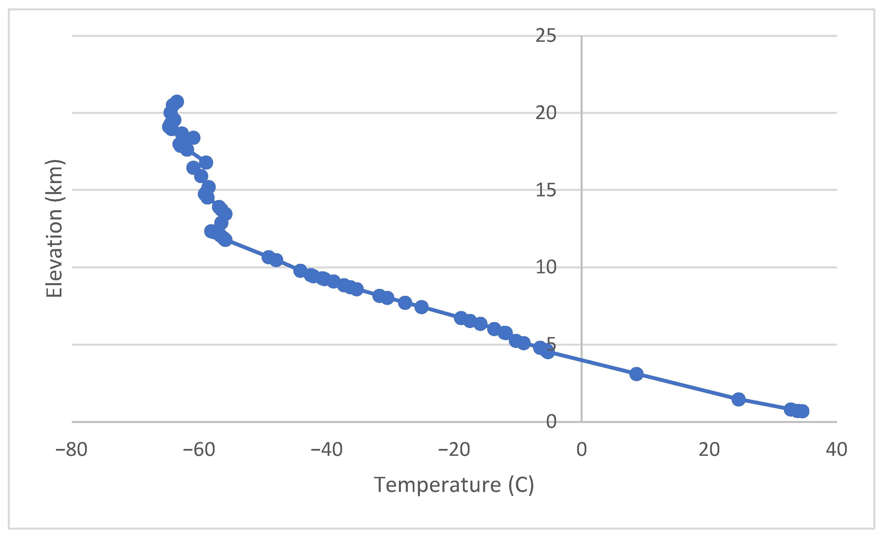
Air normally cools as altitude increases. The adiabatic lapse rate is the rate of temperature decrease with height when the temperature change with height is solely due to pressure changes. Data from radio balloon measurements was found for Las Vegas, NV for 24 May 2023 [33]. Temperature versus height is shown in Figure 1 for 0 UTC. The air temperature decreases from the ground to the top of the troposphere, which is shown here at 12,000 m.

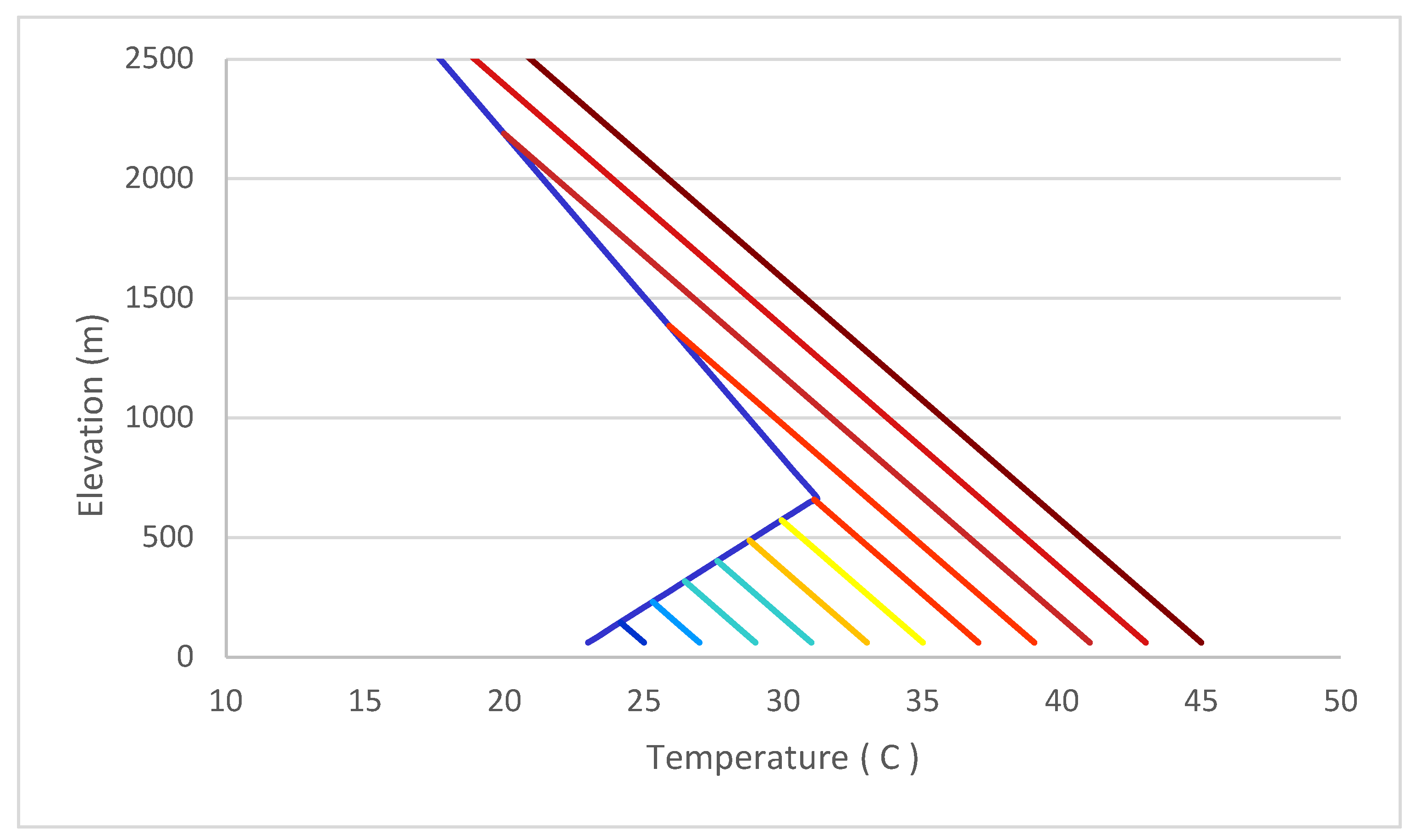
An additional factor is that air warms nonlinearly with increasing solar energy arriving at the surface. Figure 2 is a hypothetical temperature-versus-height (T-H) plot for the early mornings through mid-day. The leftmost T-H curve is the hypothetical temperature in the early morning. In that curve, the temperatures rise to the inversion, which is shown at 600 m.

In Figure 2, each curve to the right corresponds to increments in the surface temperature. As the air near the ground is heated during the day, the air above it will have to warm to the point where the line of adiabatic lapse intersects with the existing T-H curve. Figure 2 shows that incremental heating of air at the surface requires an increasing amount of thermal energy to heat the air column. The effect of this is that temperature rises rapidly in the mornings.

Non-linear heating of the air is a function of the amount of cooling the night before, the height of the PBL, and the density and humidity of the air at each level. It is complex to model it with a simple numerical equation. However, a simple model can account for the most predominant effects.

A ramp function captures the nonlinearity in the heating rate. Notice that in Figure 2, in early mornings, the heat required for each temperature increment is outlined by a triangle of increasing size. The heat required for each temperature increase goes up with the area of this triangle. Therefore, the heat required is roughly a ramp function, and the temperature change for each level of heating would ramp down:

F = 2 − t₁/13 ≥ 1

(2)

where F is the heating effectiveness factor, and t₁ is the time (hours) since sunrise. This is determined entirely empirically for the best fit under these conditions.

It will be shown that the numerical fit matches the actual temperatures when a square function is used, such that the heating rate is scaled to be double in the mornings. In the model, this is performed by including a linear ramp in the heating rate that doubles it in the mornings, but decreases to zero later. Figure 2 shows that at higher temperatures, the areas are roughly rectangular. Therefore, in afternoons, the temperature changes are roughly linear with the heating rate.

2.3. Method Details

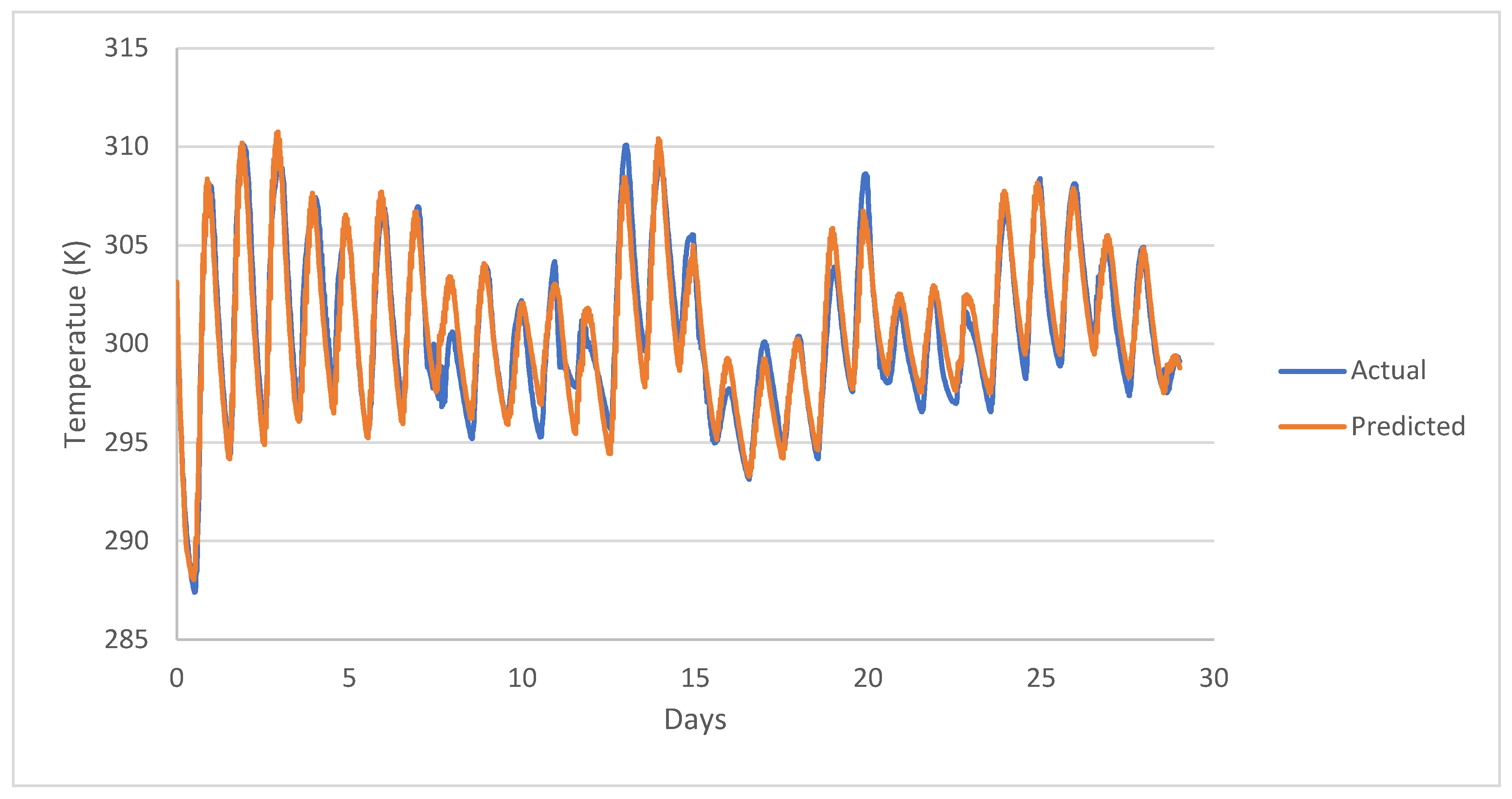
The numerical model considered the same data as the SCAM6 program. Over 29 days, all the fronts and troughs that passed through the area were found using weather maps [34]. A front or trough passed through the area every few days. There are stationary fronts on 26 June 1997 and 2 July 1997 for a few days. This is seen in the cool temperatures in Figure 3 around days 8 and 16. Stationary fronts are harder to numerically model since conditions are slowly and actively changing.

Since the frontal maps are daily, exact times for the passing of fronts are not known. Atmospheric conditions can change rapidly when a cold front passes through, but often conditions change gradually over the space of a few hours as the air mass changes. The time of passing of the front is approximated from the map. From this, modeling timelines were made by grouping together similar weather conditions. Then the groupings are finalized by confirming that the temperature data in each group appears to have the same pattern. The times for the air mass changes can be shifted a few hours if parts of a day fit better with a different grouping.

Wind varied from 0 to 38.9 m/s in the full height of the atmosphere, but in the lowest altitudes, the wind was usually below 10 m/s. The full list of data by hour and altitude are provided in http://doi.org/10.17632/n5xkn59j7h.1. The biggest effect of the wind speed is on logistics because it was assumed that higher wind requires a greater mass of calcite to maintain a constant effect on solar radiation. Therefore, it is assumed that wind has no effect on the radiation rates in the model.

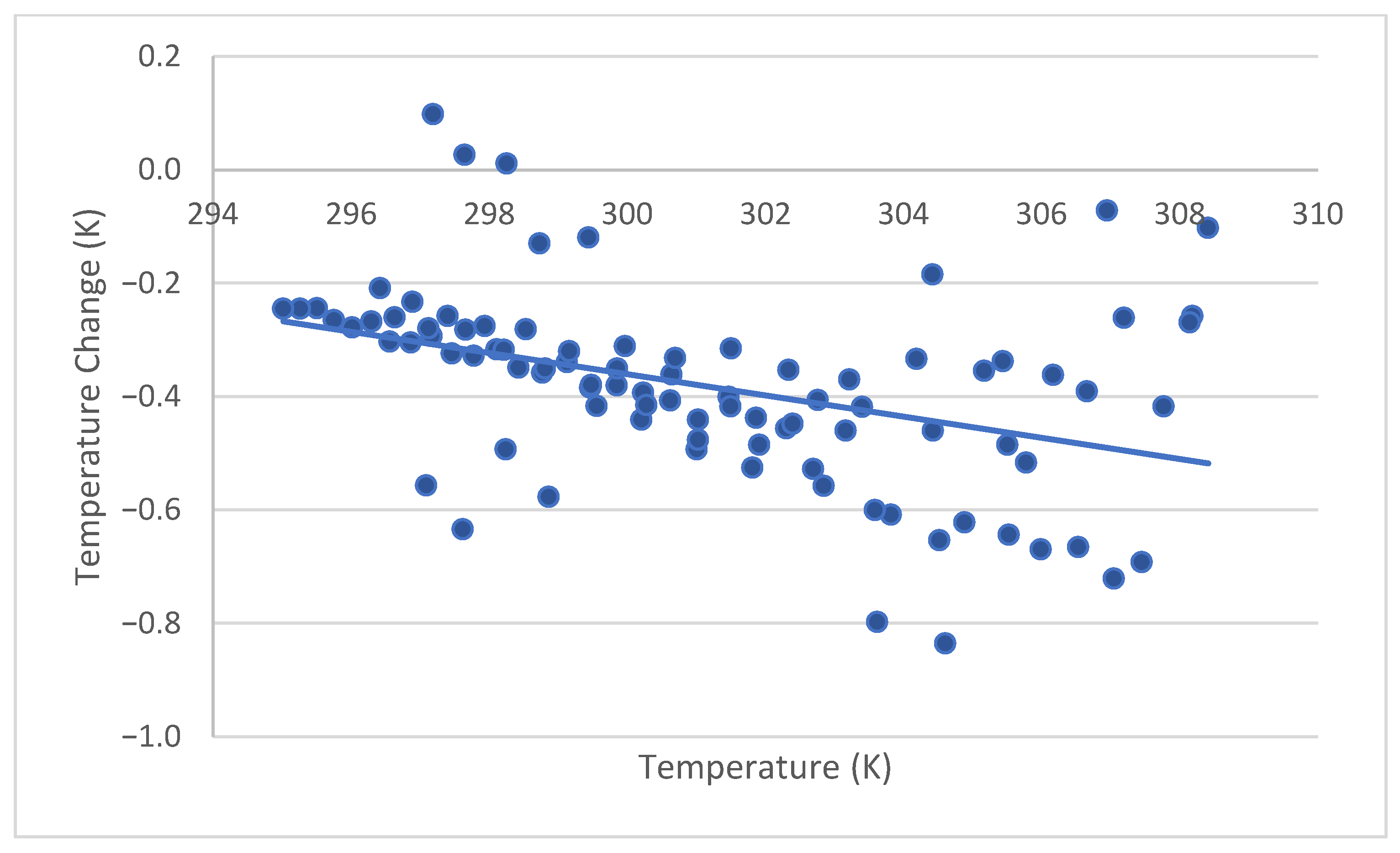
Next, for each air mass, cooling rate versus temperature is found. Figure 4 shows a sample for days 0.5 to 3.5. A weak trough passed through the area around day 3.5, but days 3.5 to 6.5 were found to have about the same cooling rates as days 0.5 to 3.5.

Figure 4 shows that the temperature changes can be bouncy while alternating from reading to reading. It is not the goal to model the apparently random bouncy changes over short time intervals. Smoothing would account for many of the unusually high or low temperature changes.

The final step in creating the numerical model is to determine the heating rate H. For days 0.5 to 3.5, the heating rate was 0.00215 degrees per watt per square meter solar radiation at the top of atmosphere. The rate was 0.00130 degrees per watt per square meter while the trough passed through day 3.5 to 4.5 and then 0.00160 degrees per watt per square meter from day 4.5 to 6.5. As mentioned previously, the rate was doubled at sunrise and ramped down to these values at later.

Cloud cover was present at various times during this model. Traditional weather reporting labels such as “partly cloudy” are insufficient to accurately model the effect of clouds on solar radiation. Instead, cloud results from SCAM6 were used. The variable CONCLD sums up the amount of condensation cloud in the air column. It was found that the model fit well to the actual temperatures on cloudy days when the CONCLD value of 1.2 was taken as reducing the solar radiation by half.

The resulting modeling equations for days 0.5 to 3.5 were:

T₁ = T₀ + ΔT_heat + ΔT_cool

(3)

ΔT_heat = 0.00215 K × I × F × (1 − 0.5/1.2 × CONCLD)

(4)

ΔT_cool = 7.13 K − 0.0250 T₀

(5)

where T₀ is the temperature in Kelvin, T₁ is the temperature one hour later, ΔT_heat is the change in temperature due to solar heating, and ΔT_cool is the change in temperature due to cooling. The time modeled was in 20-min increments because that is the CAM time. The base cooling rate is C_base and is 7.13 K for days 0.5 to 3.5, and the cooling rate is C_rate and is 0.0250 K/K per 20 min. When mitigation occurs, the solar radiation I is reduced accordingly. These calculations were performed in Excel.

Table 1. Fit factors.

Time (Days)	H (K m2/Watt)	Crate (K/K)	Cbase (K)
0.0–0.5	0.00215	−0.0409	11.22
0.5–3.5	0.00215	−0.0250	7.13
3.5–4.5	0.0013	−0.0260	7.55
4.5–5.5	0.0016	−0.0200	5.70
5.5–6.5	0.0016	−0.0250	7.21
6.5–8.5	0.0017	−0.0360	10.60
8.5–9.5	0.0012	−0.0304	8.90
9.5–11.5	0.0013	−0.0000	0.00
11.5–15.0	0.0014	−0.0193	5.56
15.0–16.9	0.0006	−0.0149	4.25
16.9–20.3	0.0011	−0.0156	4.48
20.3–23.5	0.0010	−0.0234	6.88
23.5–27.5	0.0011	−0.0230	6.75
27.5–28.5	0.0016	−0.0215	6.27
28.5–29.0	0.0007	−0.0215	6.27

shows the fit values for each time period.

A p-value < 0.001 and a 95% confidence of 3.6 K were found when comparing the numerical model to actual temperatures. A low p-value indicates that overall, the method predicts the conditions well. However, the confidence in temperature predictions shows that the numerical fit process is less useful for hour-by-hour weather prediction.

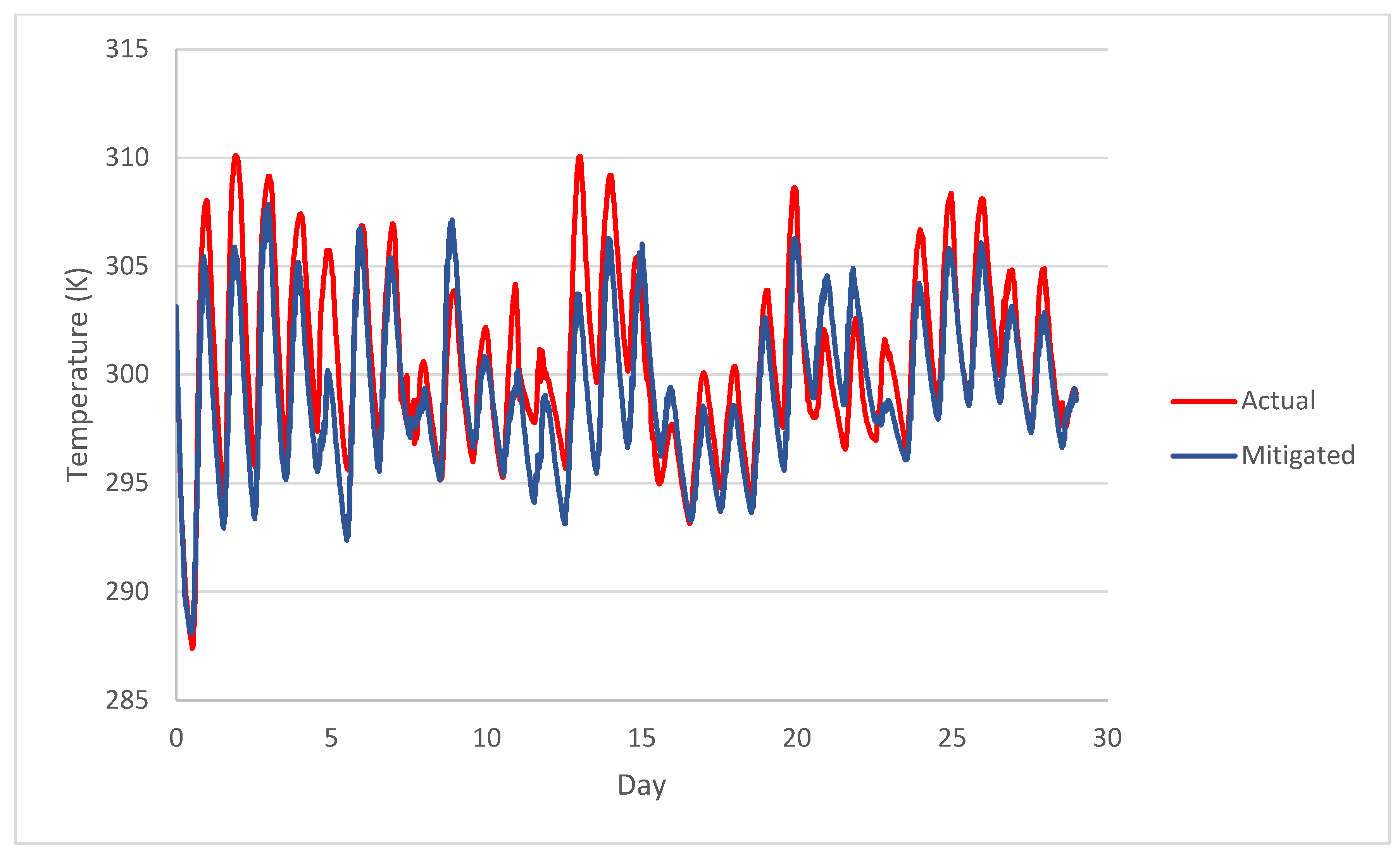
3. Results

Figure 3 shows the comparison between the actual temperatures and the numerical model. The numerical model agrees well with actual temperatures. The poorest fit is around day 8 when a stationary front is present. It would be possible to have the numerical model precisely fit the actual temperatures if it were to be fit for very short time intervals. However, the only fit factors were the heating and cooling rates for each air mass and one fit factor for the effect of the water clouds.

3.1. Mitigation

Considering that fit factors were only necessary when the air masses changed, it can be argued that the numerical model is capturing changes in heating and cooling rates. A mitigation using plumes of calcite would not significantly change the air mass locally over the city. Therefore, the same air mass heating and cooling rates can be used for mitigation cases.

During a long mitigation, ground temperatures may significantly cool. This method of modeling does not account for changes in ground temperatures.

Hoback [6] showed that interaction with water clouds significantly affected the SCAM6 modeling results in humid regions but not arid regions. To accurately check the model against results for humid regions, this interaction needed to be included. Rather than adjusting the numerical fit model to be much more complex, the solar radiation input to the numerical fit model was taken as the SCAM6 downwelling solar radiation.

Figure 5 shows the numerically predicted temperatures. Hoback [6] produced similar results using SCAM6. The days with greater cooling in one model also have greater cooling in the other. An exception is that from days 16 to 18, the SCAM6 model shows no cooling, but there is a small cooling found with the numerical fit on days 17 and 18 but a warming on day 16. The average temperature change was a decrease of 2.12 K, but for the SCAM6 model, the drop was 0.98 K for aircraft dispersal. When comparing the CAM and numerical fit results for mitigation, the p-value is less than 0.001.

A few reasons are discussed for the difference between the SCAM6 and fit models. The most significant reason may be that CAM considers horizontal advection, but the fit model does not. Advection would reduce cooling because warm air blowing into an area defeats some of the benefit. Therefore, it is reasonable to assume that the SCAM6 results would show fewer benefits. The effects of advection will be accounted for later. Since both methods show similar patterns, the numerical model can be said to be an approximation of the results from the single-column model when there is no significant water cloud interaction and if advection is accounted for. Another reason for differences is that the two models had different assumptions about whether cooling from mitigation would build up through changes in the ground temperatures.

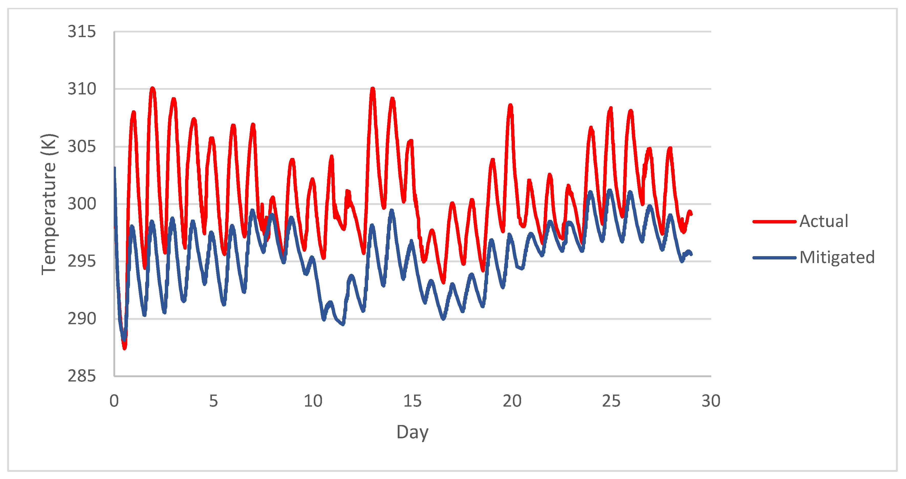
Next, an arid region was modeled with the numerical method considering that the full effect of the mitigation would be achieved. The optical depth of calcite was chosen to reduce the solar radiation by half. No interactions of the calcite with water clouds is anticipated because it is an arid location. Therefore, the heating at ground should be reduced by half due to the plume. Figure 6 shows the results of the mitigation.

The mitigation shows a dramatic drop in temperatures. The average temperatures are 6.37 K below the actual temperatures. The daytime highs are reduced by much higher amounts than the nighttime lows. In Figure 6, it is common to see a drop of 10 K during the daytime. The differences at night are usually less than 5 K. This suggests that the mitigation is well suited to reducing extreme temperatures.

3.2. Advection

The numerical fit model does not account for local horizontal advection. This was assumed to be the primary reason for the difference between the SCAM6 results and the current results.

Warm air flowing into a mitigated area will slowly adjust to a lower temperature. If lesser solar radiation has been incident on the ground from calcite plumes, the ground will slowly cool the air. A similar process occurs whenever fronts pass into a new area, and it happens at night as the ground radiates heat into space and the surface air cools. Therefore, around the edges of a plume of calcite, the numerical fit model will have a smaller benefit than predicted in Figure 6. This section is to develop a process to account for it.

Smedman et al. [35] analyzed the effects of warm continental air flowing over a cold sea. Air temperatures were simulated and compared to various aerial measurements. Heat exchange in marine environments is different than for continental areas, but the patterns are useful to understand. The simulation showed that an internal boundary layer forms immediately at the change of thermal properties. With a wind speed of 5 m/s, within 30 km, the surface wind had fully adjusted to the sea temperature. However, it took 120 km for the full height of the PBL to adjust to steady state temperatures. Higher wind speed caused the process to require longer distances.

Turbulence is a factor in the spread of heat throughout the PBL. The surface roughness of cities causes high turbulence, so it is expected that this will shorten vertical heat transfer times.

Measured temperatures in urban heat islands (UHI) at various wind speeds can be used to anticipate the effect of wind on cooled areas. Gedzelman et al. [36] correlated wind in New York City with the incremental temperatures from UHI. Below 5 m/s, the full UHI effect was observed. At twice that wind speed, the UHI effect was cut in half.

Therefore, it is expected that the benefit of mitigation will vary with wind speed. There will be a buffer distance under the edges of plumes that will vary with the wind speed. However, in typical conditions, near the center of the city, the full effect of the cooling from the calcite should be felt at the surface. In contrast, SCAM6 is a single-column model, so it finds an average temperature over a cell which smooths out temperatures. On average, the temperatures below the plume may be more similar to those found by SCAM6, but where it matters in the densely populated areas, it will be much cooler such as from the numerical fit model.

4. Discussion

Figure 5 and Figure 6 show dramatic differences in the expected temperatures depending on the region. The explanation is that the calcite plume caused a significant reduction in cloud cover in humid regions, but there are very few convective clouds in arid regions.

Hoback [6] predicted these results by extrapolating adjustments to the humidity and cloud cover. It was found that when there were fewer condensation clouds at low altitudes, the interaction with clouds decreased. Incremental reduction in humidity increased the performance of the mitigation. Eventually, with low humidity, there was no interaction with clouds. This shows that plumes of calcite are much more effective in areas of lower humidity.

Other methods of solar radiation management have a much lower local effect because they are intended to reduce average global temperatures. Stratospheric aerosol injection with sulfur could have an effect of 3.71 W/m² [37]. Small-scale experiments with MCB have achieved about 1 W/m² [38]. In comparison, the models show that mitigation with calcite at low altitudes can regularly reduce solar radiation by 100 W/m². However, it has only local effects, so it does not mitigate climate change globally; rather, it reduces the urban heat island effect in cities.

Other strategies for the mitigation of urban heat islands can reduce temperatures. Planting a dense canopy of trees in Montreal could reduce air temperatures by 4 C [39]. This is significantly less than the projected improvements for arid cities in Figure 6, but it matches the results for humid cities as shown in Figure 3. A full canopy of trees mitigates air temperatures in the immediate vicinity, but it does not have a significant effect on the solar heat gain felt in buildings.

A limitation of the modeling approach is that it is difficult to use for prediction of future weather. The numerical fit method uses historical data. Therefore, it is only a theoretical tool for evaluating scenarios. A bias would occur if it was applied to the future if it was assumed that the air mass properties would stay the same for the future.

Further validation of this work can be carried out with experimental methods. Also, surrogate data sources can be used. It is well documented that water clouds reduce solar radiation and temperatures. However, a complication is that clouds are correlated to changing atmospheric conditions as air masses change. Aerosols have varying effects on air temperatures depending upon the source of the aerosol. High temperatures increase the likelihood of dust storms [40]. Therefore, any correlations between temperatures and naturally occurring dust can confuse cause and effect. It would be difficult to isolate the effect that natural dust has on temperatures.

Experimental validation should be explored through application of the design of experiments methodology. One of the challenges will be real-time validation. In addition to standard meteorological data, during experimentation and implementation, it may be necessary for aircraft to collect aerial data about numerous factors such as solar radiation rates and dust plume elevations and concentrations. This may result in on-the-fly modification of procedures.

5. Conclusions

The goal was to show that numerical fit can be an alternative to more complex analysis. This was needed because only a few cases had been developed, and they were all in humid regions.

Key results were that (1) the numerical fit procedure discussed in Section 2 can model air temperature changes when plumes of calcite are placed above cities, (2) the numerical fit procedure and the supercomputer model of the previous work produce similar results, but the supercomputer results show lower changes in temperature, (3) the differences in temperatures between the methods are due to variations in how advection is handled, and (4) both methods have advantages with the supercomputer method representing an average and the numerical fit representing the peak benefit in the core urban area of the city.

Calcite reflects shortwave radiation more efficiently than longwave radiation, so as an aerosol it is effective at cooling the ground surface. Plumes of calcite can reduce temperatures in cities.

Placing calcite in the atmosphere in any region will reduce solar radiation. The amount of reduction may be lower in humid areas.

A numerical fit model was created that estimated temperatures with simple equations for heating and cooling rates. The model needed tuning whenever a new air mass entered the study area because the properties of the air changed. The fit model produced results similar to those of a SCAM6 model by Hoback [6] but with bigger temperature changes expected. A benefit of the numerical fit method is that it uses actual temperatures, so it can be used for weather forecasting during a mitigation. Accounting for advection in the numerical fit model makes it similar to the results from SCAM6, but the results vary geographically. Further, under the plume of calcite, the temperatures become less affected by advection and so would approach the results from the numerical fit model.

In arid regions, there is much less interaction of aerosols with clouds, so the analysis of temperature changes can be more simply modeled. The SCAM6 cases are not available in arid regions, so the numerical fit model should be applied. To apply this to humid regions, existing data about cloud interaction are necessary.

For each city where this is applied, a new model must be created. The heating and cooling rates vary by geography. The methods are generalizable to other arid cities, but the results are not. Section 3.1 illustrates that this method can be applied to humid cities. However, it was necessary to have extensive data about the clouds that were present. This is more data than are found in weather reports. Therefore, to apply this to humid cities requires a modification to account for clouds such as CONCLD or other equivalent data.

Several economic, health, social, and ecological issues should be considered. Those are outside of the scope of this paper.