Transformation of Hydroacoustic Energy into Seismoacoustic Energy at 22 Hz in Medium Depth- and Deep-Sea Conditions

Abstract

This work is devoted to an experiment studying the regularities of the propagation of hydroacoustic low-frequency signals in the conditions of the sea at intermediate depth and deep in terms of their transformation into vibrations in the upper layer of the Earth’s crust. This experiment belongs to the field of acoustic tomography and is aimed at solving the problems of non-contact methods for studying the geological structure of the shelf areas of the World Ocean. The novelty and uniqueness of the work lies in the use of a harmonic low-frequency hydroacoustic signal with a frequency of 22 Hz of high power, capable of creating Rayleigh surface waves at the “water–bottom” interface. The surface waves propagating at the bottom are registered by a coastal laser-interference measuring system capable of recording deformations in the upper crustal layer with an accuracy of 0.01 nm. The experimental results showed that the radiated hydroacoustic energy is not localized in the liquid half-space and propagates predominantly according to the law close to spherical divergence, even when the shelf depth is comparable to the wavelength of the radiated signal.

1. Introduction

Acoustic tomography methods have been developed for monitoring marine environment parameters in large- and deep-water areas. The method consists of detecting hydrophysical processes and anomalies by fluctuations in the parameters of the acoustic signal traveling from the radiation source to the receiver. The advantage of this method is that it is possible to cover large areas and volumes of the water column, which has an undeniable advantage over point measurements. However, recently, with the development of the shelf areas of the World Ocean, the tasks of monitoring the parameters of the shallow sea, where the bottom parameters can strongly influence the obtained results, especially in the conditions of a wedge-shaped shelf, are of great interest [1]. In this connection, another task arises, namely, the determination of the geologic structure of the upper layer of the marine crust.

Currently, the most common solution to this problem is the use of specialized vessels with towed acoustic antennas and seismic streamers, but their use has its limitations, for example, in the conditions of water areas covered with ice. Recently, to study the structure of the upper layers of the Earth’s crust and their characteristics, the method of emission seismic tomography has been used. This method is passive. Information about the structure and state of the environment is obtained by recording seismic noise from endogenous sources. However, although this type of tomography has great prospects, it has so far only proven itself in the discovery of minerals in limited areas [2].

One of the promising tools for the remote investigation of both inhomogeneities in the ocean and diagnostics of rocks of the ocean floor in shelf regions is low-frequency hydroacoustics. When powerful low-frequency hydroacoustic signals are used, some of the energy penetrates the seafloor and propagates as seismoacoustic and surface waves. In most sources, the use of such signals to determine seafloor parameters from geoacoustic modeling and in situ measurements is referred to as geoacoustic inversion. When solving these problems, it is necessary to know the diagnostic signals’ propagation patterns in various media, in this case, in the water, air, and seabed. Taking into account the media impedance, we can state that in the case of radiating in water, we will be interested in only two media—water and the upper layer of the marine Earth’s crust. It is in these media that the main radiated hydroacoustic energy will propagate. It is important to know the propagation patterns of these hydroacoustic signals, which are mainly associated with the frequency dependences of these patterns on the size of the inhomogeneities in the propagation media.

Both theoretical studies [3,4,5] and in situ measurements [6,7,8] can be used for studies related to the regularities of signal propagation and the formation of acoustic fields in liquid and solid half-space. At the same time, other complex problems such as ocean thermometry and the location of and communication with underwater objects located in the water space and on the seabed can be solved in parallel [9,10,11].

In the water environment, the depth of the sea and the size of the near-surface channel play the main role [12]. It is clear that with a decrease in the frequency of the radiated signals, the axis of the sound channel plays a smaller role, and at certain frequencies, the boundary of the density jump can be transparent for the radiated signals. It is clear that in this case the main radiated hydroacoustic energy will propagate both in the water and move into the seabed in the form of volumetric seismoacoustic waves; it also propagates in the form of attenuating and unattenuating surface waves of Rayleigh type along the “water–bottom” boundary. When solving tomographic problems, it is important to know the relationships of all the components propagating in the water media, at the bottom and at the “water–bottom” boundary. These relationships are especially interesting when performing works on a shelf of monotonously decreasing depth and when operating radiators that generate signals of varying complexity in the low-frequency audio range.

In recent years, we have conducted experiments using low-frequency hydroacoustic signals of various frequencies, which allowed us to better understand the patterns and mechanisms of formation of the acoustic field on the shelf, as well as the transfer of energy from the liquid to the solid half-space and vice versa. These studies were carried out using a complex [13] consisting of coastal laser-interference measuring systems recording seismic signals and low-frequency acoustic radiation systems of 22, 33, and 245 Hz. In addition, for measuring the characteristics of the acoustic fields created by the radiators, the complex includes several autonomous receiving systems with hydrophones.

Thus, one work [14] describes an experiment on the emission of harmonic signals with a frequency of 33 Hz, generated by a low-frequency hydroacoustic radiator in Vityaz Bay, which, having passed along the shelf of decreasing depth and having transformed into seismoacoustic signals of the upper layer of the earth’s crust and bedrock of Shultz Cape, excited hydroacoustic signals at the corresponding frequency in the waters of the shelf of the open part of the Sea of Japan. The experimental data were compared with a model, constructed taking into account the geological structure of the water areas, as a result of which the mechanisms of the transformation of hydroacoustic energy into seismoacoustic and back were described.

In [15], we considered some patterns of hydroacoustic signal generation in the bay, the depth of which is comparable to half the wavelength of the radiated harmonic hydroacoustic signal (22 Hz wavelength of about 68 m). When studying the patterns of radiated hydroacoustic signals transformation into seismoacoustic signals at the corresponding frequencies recorded by the laser strainmeter (V.I. Il’ichev Pacific Oceanological Institute, Far Eastern Branch, Russian Academy of Sciences, 690041 Vladivostok, Russia) located at Shultz Cape in the Sea of Japan, we believed that the laser strainmeter registered mainly surface Rayleigh waves, which propagate in water, along the “water–bottom” boundary, and on land—along the “Earth’s crust–air” boundary. In the described case, the sea depth is approximately two times smaller than the length of the hydroacoustic wave. This is a special case of hydroacoustic signal generation, in which the elastic bottom plays a certain role in the value of the radiated hydroacoustic signal’s amplitude. The considered case is not entirely typical when performing such hydroacoustic work. Carrying out further work in this direction, we are interested in cases where the sea depth is comparable to, greater than, and significantly greater than the length of the hydroacoustic wave. Similar experiments have been conducted; their results are described in this paper, with detailed interpretation of the obtained experimental data processing results.

2. Experiment

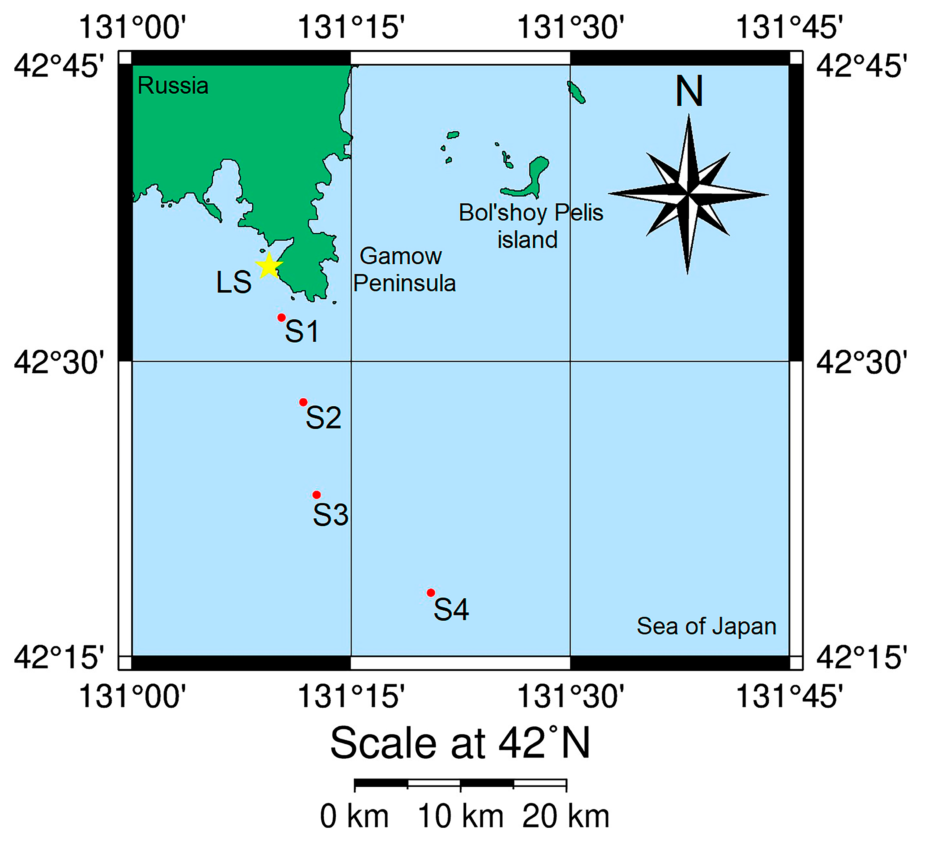
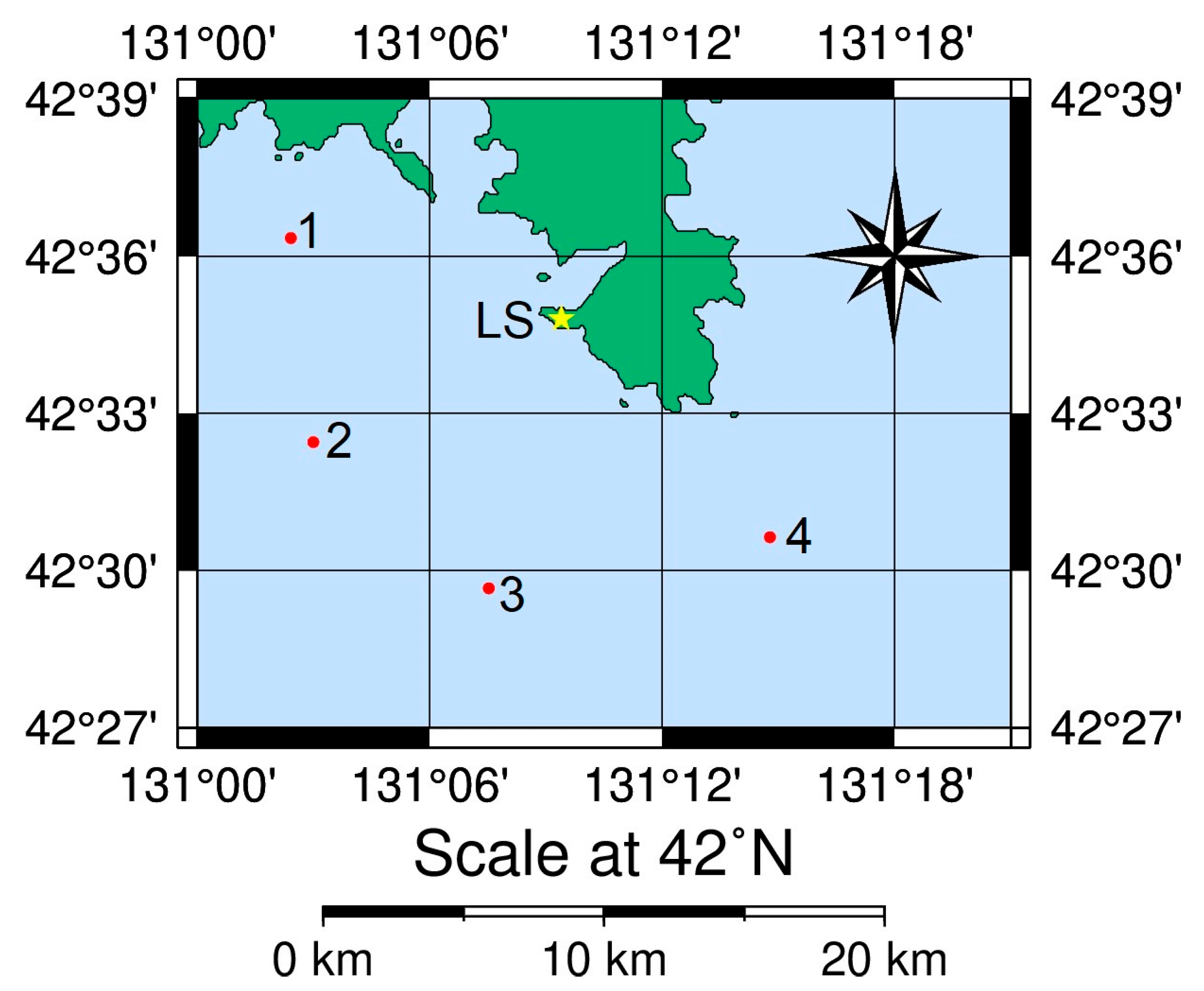
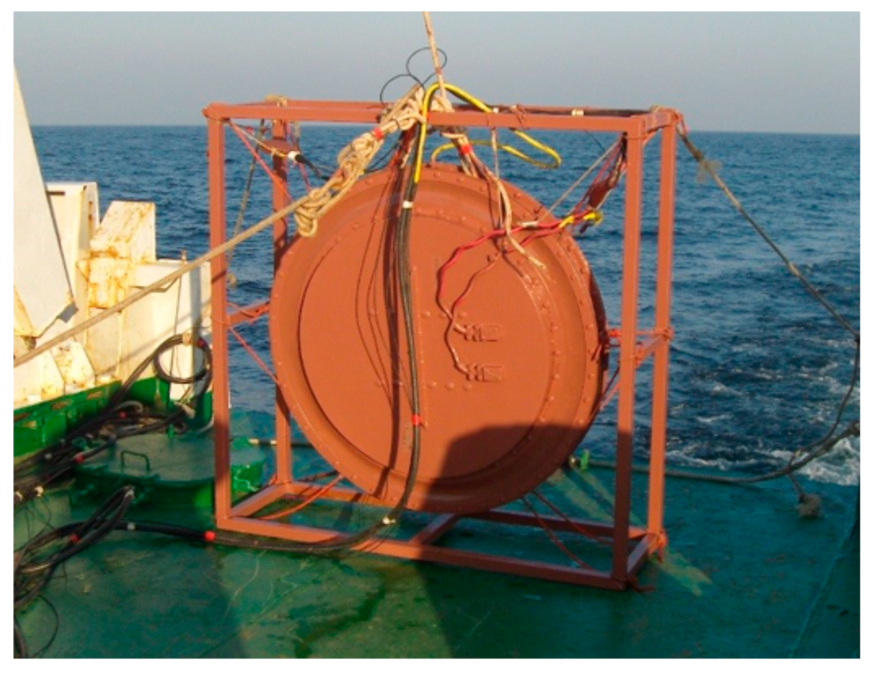
Figure 1 shows a map scheme of the experiment. A low-frequency hydroacoustic radiator operating at frequency of 22 Hz [16] was submerged from the “Akademik Oparin” research vessel to the depth of 18 m. The radiator is a part of radiating hydroacoustic system consisting of a radiator with an electromagnetic transducer, a frame for suspending the radiator, a cable-hose with a control manometer, a power source, an electric pump, a control hydrophone, and two calibration accelerometers. The radiating hydroacoustic system is designed to generate harmonic and phase-shift keyed hydroacoustic signals in the frequency band of about 1 Hz in the range of 19–26 Hz. The amplitude of the volumetric oscillatory displacements of the radiator reaches 0.0123 m³. At the frequency of 20 Hz in the limitless water area, this corresponds to a radiated acoustic power of 1000 W. The exterior view of the radiating hydroacoustic system is shown in Figure 2. During operation at each station, the low-frequency hydroacoustic radiator created pressure of about 7 kPa, which was registered by the control hydrophone.

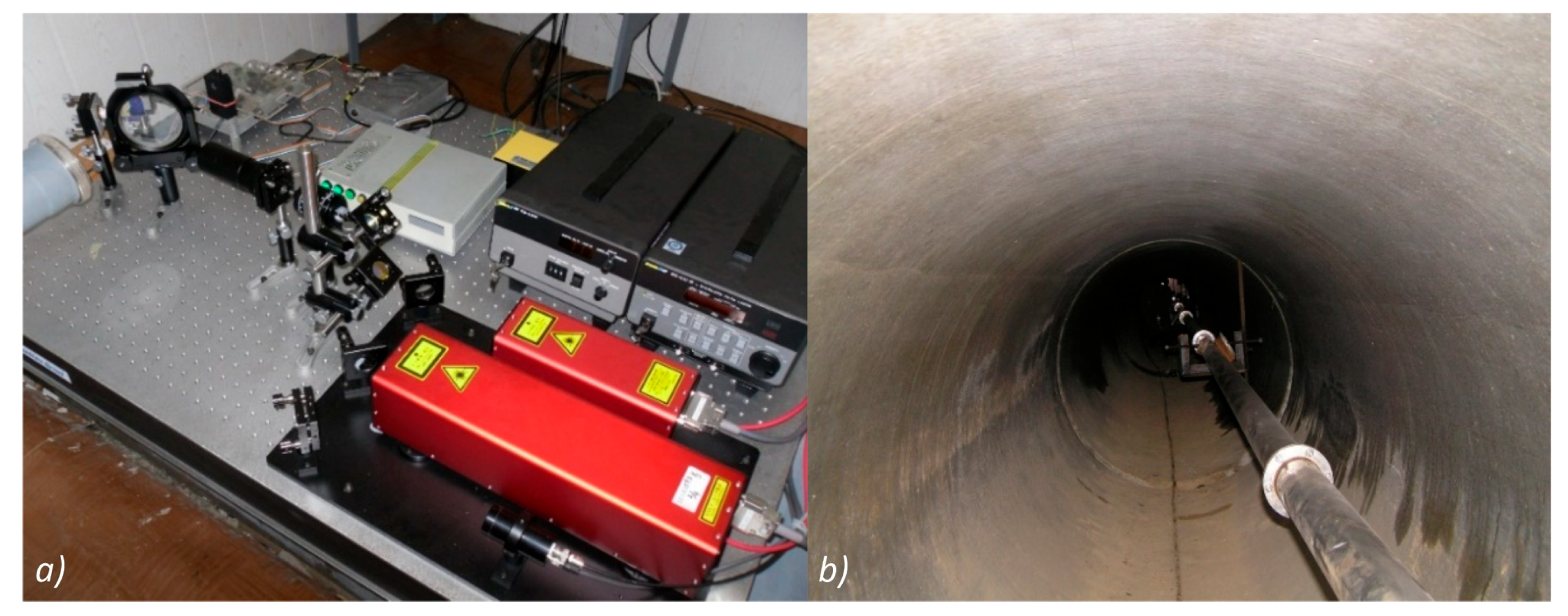
The seismoacoustic signal was recorded by the 52.5-meter laser strainmeter located on Shultz Cape. The laser strainmeter is installed at N42°35.5817′, E131°09.9667′ on Shultz Cape underground, at a depth of 3–5 m from the ground surface, in specially built underground hydro-thermally insulated rooms that ensure satisfactory temperature stability; see Figure 3. Operation of the laser strainmeter is described in [17]. The part of the 52.5-m laser strainmeter structure closest to the water (corner reflector) is located at the distance of 120 m from the water edge and at 67 m above sea level. The working arm of the 52.5-m laser strainmeter is oriented at the angle of 18° relative to the north–south line. All information from the laser strainmeter’s registration system is sent via cable lines to the laboratory building, where it is entered into a specially created database. The obtained experimental datasets are then subjected to preliminary and final processing, depending on the set tasks. The interferometry methods used in the laser strainmeter allow measuring changes in the intensity of the interference pattern with high accuracy. Theoretically, using interference methods, it is possible to measure the displacement between the strainmeter plates with an accuracy of ${10}^{-6}\times {\displaystyle \frac{{\lambda }_l}{2}}$, where ${\lambda }_l$ is the wavelength of the used frequency-stabilized laser. In our case, the accuracy of measuring the displacement between the plates is 0.01 nm.

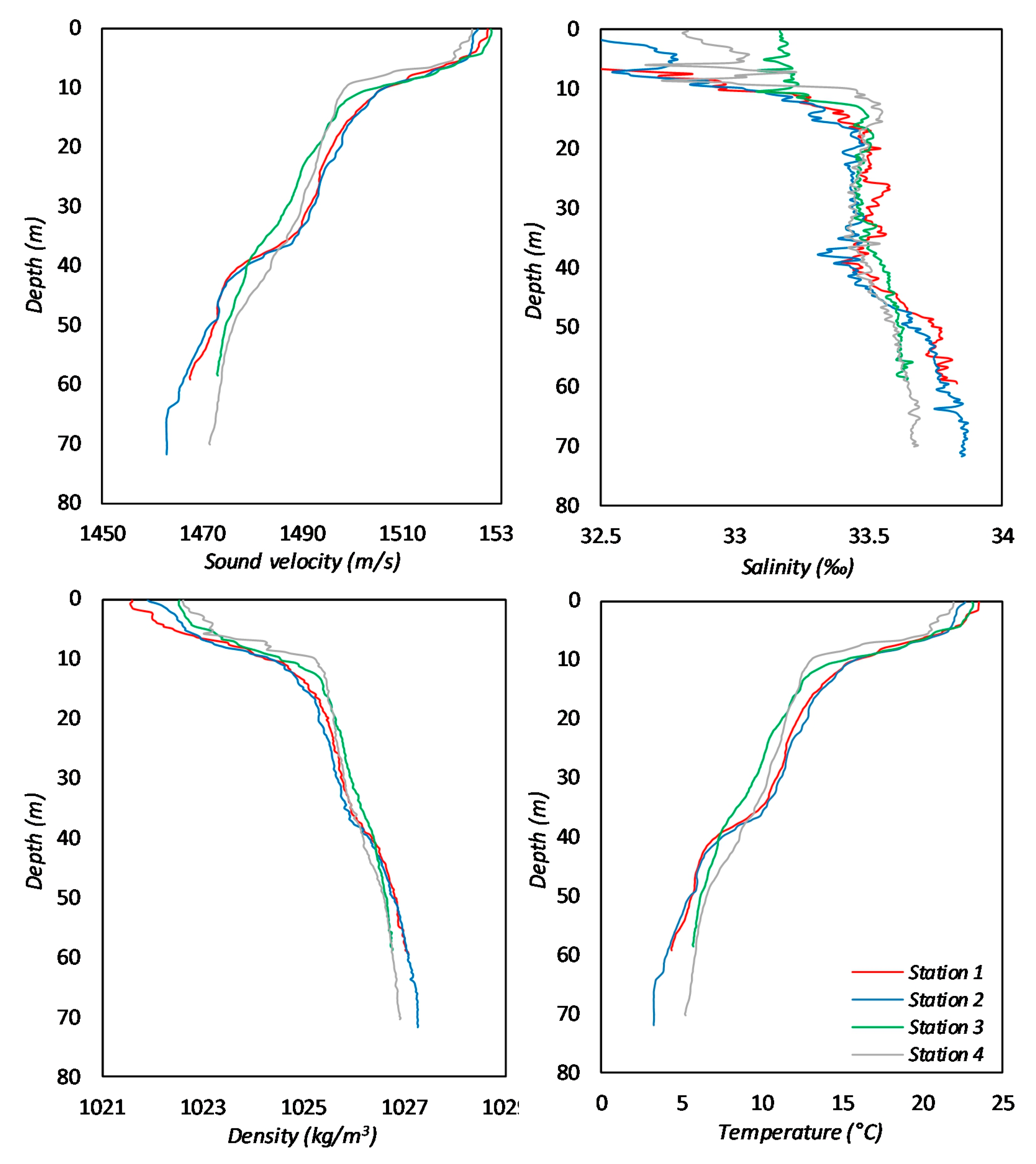
Also during the experiment, in each radiation station, hydrological parameters of the environment such as the temperature, salinity, density, and sound velocity were measured. The purpose of these measurements was to identify sound channels and inhomogeneities of the medium, affecting the sound propagation.

The obtained experimental datasets at the end of the experiment after preliminary processing were placed in the experimental database for further processing and interpretation of the results.

3. Description of the Obtained Results: Processing and Interpretation

Table 1. Data on radiation stations.

Station	21.07.2024, UTC	Latitude, N	Longitude, E	Azimuth, deg	Distance, m	Depth, m
1	Start—04:56	42°32.214	131°10.243	166.56	4926	52
	End—05:07	42°32.318	131°10.256	165.98	4742
2	Start—06:29	42°27.915	131°11.728	166.09	13,146	74
	End—06:38	42°27.995	131°11.710	165.99	12,996
3	Start—08:04	42°23.222	131°12.650	168.34	21,908	108
	End—08:13	42°23.368	131°12.641	168.24	21,641
4	Start—18:06	42°18.238	131°20.468	153.31	34220	1500
	End—18:15	42°18.275	131°20.518	153.21	34,189

shows some data on the radiation stations: the first column contains the radiation station number; the second column contains the radiation start and end time, UTC; the third column contains the latitudes of the radiation’s start and end; the fourth column contains the longitudes of the radiation’s start and end; the fifth column contains the azimuth of the laser strainmeter axis at the radiation’s start and end; the sixth column contains the distance from the radiation point to the laser strainmeter at the radiation’s start and end; and the seventh column shows the average sea depth at the radiation station according to the echo sounder (except for station 4, determined from the map).

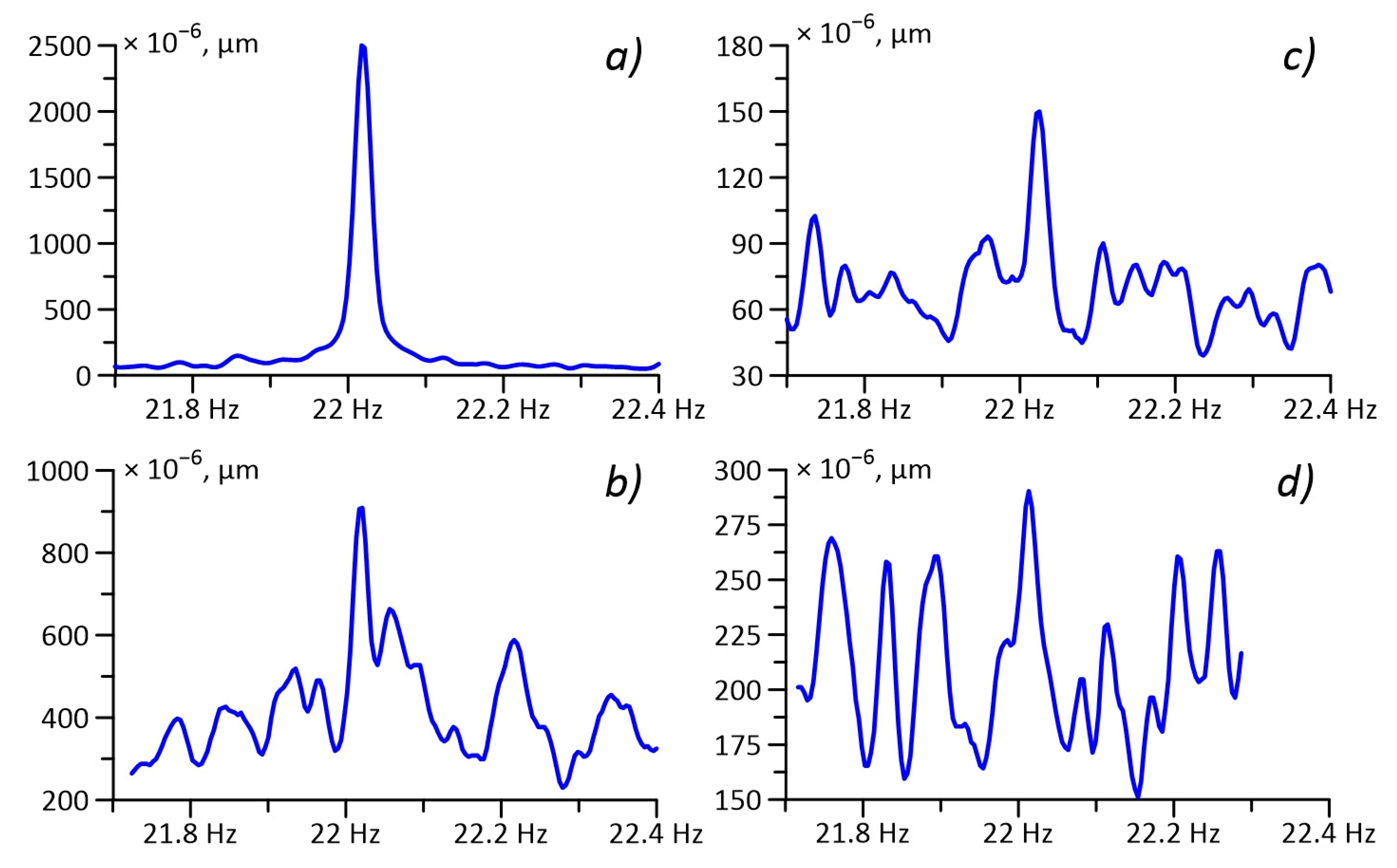
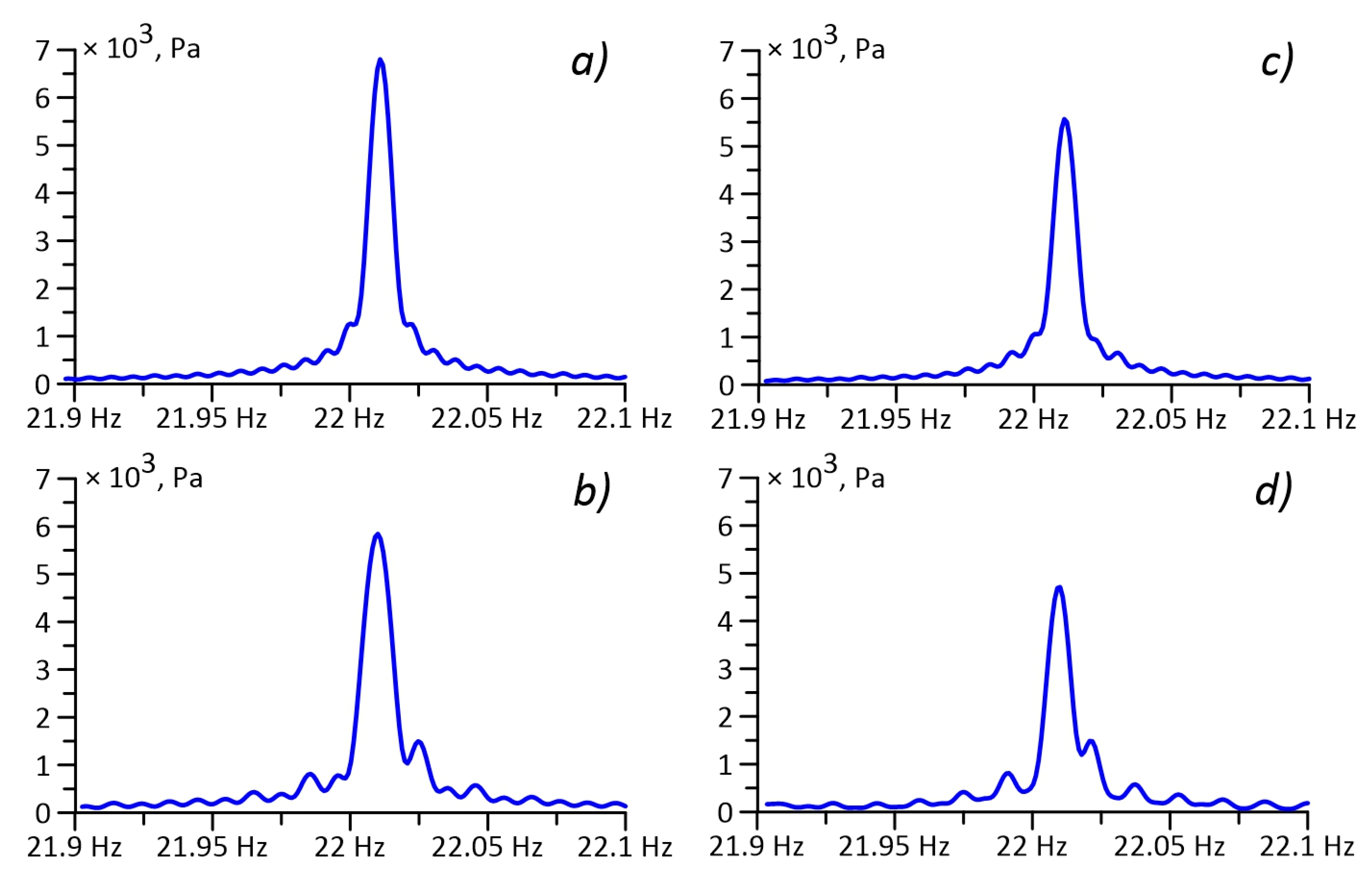
For further processing, we used experimental data obtained on the 52.5-m laser strainmeter. Processing was carried out using standard spectral methods; with their help we determined the amplitude of the registered signal at the radiation frequency during operation of the low-frequency hydroacoustic radiator at each station. Figure 4 shows fragments of spectra with the maxima at a radiation frequency of 22 Hz.

In our further calculations, in accordance with [15], we assume that the laser strainmeter records a Rayleigh-type surface wave formed as a result of the transformation of a hydroacoustic wave at the “water–bottom” boundary and propagating along “the Earth’s crust–air” boundary. We use the following data in our calculations: ${\rho }_w=1000 \mathrm{kg}/{\mathrm{m}}^3$ (water density), $c_w=1500 \mathrm{m}/\mathrm{s}$ (sound speed in water), ${\rho }_b=2100 \mathrm{kg}/{\mathrm{m}}^3$ (density of the rocks of the upper layer of the Earth’s crust), $c_b=2300 \mathrm{m}/\mathrm{s}$ (Rayleigh-type wave speed at “the Earth’s crust–air” boundary), $f=22 \mathrm{Hz}$ (frequency), $\theta$ is the angle between the laser strainmeter axis and the “radiator-stations 1, 2, 3, 4” line, $\omega =2\pi f$, and $R$ is the average distance from the radiation point to the nearest point of the laser strainmeter. For a Rayleigh wave, the amplitude decays exponentially with the depth of the Earth’s crust. The elastic energy density of Rayleigh-type surface waves can be calculated using the following equation [15]:

$$E_r={\int }_0^{{\lambda }_b}{\displaystyle \frac{{\rho }_b{\omega }^2{u}^2\exp (-4\pi z/{\lambda }_b)}{2\cos (\theta {)}^2}}dz,$$

(1)

where $u$ is the amplitude of the displacement at the frequency of the radiated signal, and ${\lambda }_b$ is the Rayleigh wavelength at the “air–the Earth’s crust” boundary, equal to 104.5 m.

In this work, it is fundamentally important to determine what laws will be used to propagate the energy from the radiation source to the receiving point. In particular, we are interested in the laws of energy attenuation, by which we can judge the processes of transformation of the acoustic into the seismoacoustic field. In this case, we consider the spherical and cylindrical divergence. For this experiment, the conditions of cylindrical divergence should correspond to stations 1, 2, and 3, since the depth of radiation is less or commensurate with the wavelength of the radiated signal (68 m). This means that the formation of the acoustic field will be influenced by the bottom, most of the energy will be concentrated in the liquid half-space, and its attenuation will be proportional to the square root of the distance to the receiving point. At radiation station 4, the depth is many times greater than the wavelength, respectively, and a free acoustic field will be formed, which is less affected by the seabed. In this case, we can talk about spherical divergence, and the attenuation will be proportional to the distance from the radiation source to the receiving system. Knowing the seismoacoustic energy density at the receiving point and the distance to the radiator, we can recalculate the energy density at the point of radiation according to the cylindrical and spherical divergence and compare them. The calculation results are summarized in

Table 2. Densities of seismoacoustic energy at the receiving point and at the emission points considering cylindrical and spherical divergence.

Station	Displacement, nm	Seismoacoustic Energy Density, J/m2	Distance to Source, m	Seismoacoustic Energy Density with Regard to Cylindrical Divergence, J/m2	Seismoacoustic Energy Density with Regard to Spherical Divergence, J/m2
1	2.5	$1.44\times 10^{-9}$	4834	$6.96\times 10^{-6}$	$3.4\times 10^{-2}$
2	0.91	$0.194\times 10^{-9}$	13,071	$2.5\times 10^{-6}$	$3.3\times 10^{-2}$
3	0.15	$0.0047\times 10^{-9}$	21,774	$0.1\times 10^{-6}$	$0.2\times 10^{-2}$
4	0.29	$0.028\times 10^{-9}$	34,204	$0.96\times 10^{-6}$	$3.3\times 10^{-2}$

.

Analyzing the results of the calculations given in Table 2, it becomes clear that we did not obtain the exact results we expected. It would be logical to assume that if the acoustic energy at each point of radiation is the same, then, when recalculated taking into account the cylindrical divergence, we should have obtained the same values of energy density at stations 1–3, and at station 4, the energy should have been different from all the others. However, considering the results, given in the last column of the table, we see that the energy (energy density) spreads from the emission site at each station to the laser strainmeter according to spherical laws, i.e., it is not localized in the liquid half-space. It can also be seen that the values of the energy density at station 3 are much smaller; we consider in detail the reasons for this in the discussion.

In order to be convinced of the correctness of the conclusions, let us consider one more experiment. Unlike the experiment presented above, the radiation was conducted at different points, at the same distance of 10 km from the laser strainmeter. The scheme of the experiment is presented in Figure 5.

The coordinates of the radiation stations and the distance from the measuring systems are presented in

Table 3. Coordinates of radiation stations and distance from laser strainmeters.

Station No.	Coordinates of the Radiation Stations	Distance from LS, km	Azimuth, deg
1	N 42°36′20.3″, E 131°2′25.3″	10	283.85
2	N 42°32′26.9″, E 131°2′59.9″	10	240.95
3	N 42°29′39.4″, E 131°7′31.7″	10	198.18
4	N 42°30′37.9″, E 131°14′47.3″	10	134.41

.

We calculate the energy densities using the same algorithm as for the first experiment. The calculation results are given in

Table 4. Calculation results based on the obtained data.

Station	Displacement, nm	Seismoacoustic Energy Density, J/m2	Distance to Source, m	Seismoacoustic Energy Density with Regard to Cylindrical Divergence, J/m2	Seismoacoustic Energy Density with Regard to Spherical Divergence, J/m2
1	0.71	$1.6\times 10^{-8}$	10,000	$1.6\times 10^{-4}$	$1.6$
2	0.87	$0.236\times 10^{-9}$	10,000	$2.36\times 10^{-6}$	$2.36\times 10^{-2}$
3	1.36	$0.31\times 10^{-9}$	10,000	$3.1\times 10^{-6}$	$3.1\times 10^{-2}$
4	1.00	$0.84\times 10^{-9}$	10,000	$8.4\times 10^{-6}$	$8.4\times 10^{-2}$

.

Based on the calculation results from Table 4, we can see a good agreement of the values of seismoacoustic energy densities at stations 2 and 3 with the first experiment. However, there are differences at stations No. 1 and No. 4, which we discuss below.

Usually, in our experiments, to quantify the transformation of energy from hydroacoustic to seismoacoustic, we measure the vertical distribution of the pressure field along the signal propagation path at several points. In the experiment, described in [15], such a measurement was made at a point at a depth of 37 m, 335 m from the radiator, and the energy density calculated from the obtained values was 0.176 J/m². Of course, this value is an order of magnitude larger than the values obtained in this work, but it confirms our earlier conclusions that the energy (energy density) propagates from the place of radiation at each station to the laser strainmeter according to the spherical law or close to it.

4. Discussion of the Results

As noted above, in the first experiment at station 3, the values of the upper crustal layer displacements were obtained at an order of magnitude lower than for the other stations. To explain this effect, we can make several assumptions. The most logical explanation for this may be that for some reason the acoustic energy does not pass into the bottom and remains in the liquid half-space. First of all, this could be due to the instability of the radiator. At each emission station, during the first experiment, we monitored the parameters of the emitted hydroacoustic field using a control hydrophone located 1 m from the acoustic axis of the radiator. The spectra of the recording of the control hydrophone are shown below, when the radiator is operating at each of the stations (Figure 6).

As can be seen from Figure 6, the radiator worked stably. There was a noticeable decrease in the amplitude of the signal at each of the subsequent stations. We associate this effect with an increase in the depth of the radiation stations: the greater the depth, the more acoustic energy goes into the aquatic environment, and the less energy remains in the near field of the radiator. Another reason may be a slight discharge of the accumulator batteries from which the radiator is powered, but this is unlikely and does not explain the low level of the seismoacoustic signal at station No. 3.

The reason for the concentration of hydroacoustic energy in the water may also be related to the hydrological conditions during the experiment. In paragraph 2, we mentioned that during the experiment, measurements of hydrological parameters were made in each radiation station; their graphs are presented below (Figure 7).

We can see from the presented graphs that, for the salinity, density, sound velocity, and temperature, there is a sharp change in behavior at depths in the range of 10–13 m. The radiator was submerged to the depth of 18 m, which was 5–8 m lower than the density jump. Considering that the wavelength of the radiated signal is significantly greater than these depths, we can state that such changes in hydrological parameters did not have a significant effect on the formation of a hydroacoustic wave at the frequency of 22 Hz (the frequency of the radiated signal).

Let us try to explain this behavior by the peculiarities of the hydroacoustic energy transformation into seismoacoustic in the conditions of a wedge-shaped shelf. In the conditions of the deep sea, the main loss in sound propagation is the medium itself. However, when passing the hydroacoustic signal to depths commensurate with the wavelength, the influence of the bottom increases. As the depth of the sea decreases, the fraction of energy that is released from the water layer to the sea bottom increases, passing into elastic vibrations of the water–bottom interface and seismoacoustic waves of the bottom soil of longitudinal and transverse polarization. According to [13], the density of energy transferred into elastic surface and volume waves at a point of a plane waveguide can be written as

$$\epsilon (x,z)={\displaystyle \frac{{[P(x,z)]}^2}{2\rho c^2}}={\displaystyle \frac{2P_0^2}{\rho c{H}^2{(f_0^2-f^2)}^{\frac{1}{2}}x}}{\sin }^2(\alpha z){\sin }^2(\alpha z_1)e^{-{\displaystyle \frac{4\pi }{c}}{(f_0^2-f^2)}^{{\displaystyle \frac{1}{2}}}x},$$

(2)

where H is the depth of the sea, P₀ is the acoustic pressure at the radiation point, α = 2πf₀/c is the vertical wave number, z is the depth at the measurement point, z₁ is the depth of the radiation source, ρ is the density of the medium, c is the speed of sound, f is the frequency of the radiated signal, and f₀ is the critical frequency, described by the expression

$$f_0={\displaystyle \frac{c}{4H\sqrt{1-n^2}}},$$

(3)

where n is the refractive index, equal to the ratio of the sound speed in water (c) to the sound speed in the sea bottom.

From expression (2), it can be seen that the maximum of the energy transferring to the solid half-space will be reached at f = f₀. Thus, from (3), each critical frequency will correspond to its critical depth H, at which the energy will be completely transferred to the elastic vibrations of the bottom. It follows from the above that the hydroacoustic signal should propagate in the water along the shelf and, when reaching the critical depth corresponding to its frequency, should completely transfer into seismoacoustic oscillations. In our case, the critical depth for the 22 Hz frequency is 34 m, which explains well the large amplitudes of the seismoacoustic signal at stations No. 1 and No. 2 in the first experiment, since the hydroacoustic signal is practically not delayed in the water and quickly reaches the critical depth, after which it is completely transformed into elastic vibrations of the bottom. However, this does not explain in any way the sharp decrease in the amplitude at station No. 3 and its reverse increase at station No. 4.

Thus, we are left with the only rational explanation of this phenomenon, namely the influence of the bottom relief and its geological structure at station No. 3. Several assumptions can arise here. The first of these is that, due to the complex relief of the seabed, there was an absorption of the hydroacoustic energy due to its dissipation during propagation, with only a small part of the energy transferred to the surface and seismoacoustic waves. In the second case, it can be assumed that, due to the geological structure of the seabed at this station, most of the hydroacoustic energy passed through the sedimentary rocks up to the granite base and propagated bypassing the laser strainmeter.

Let us return to the second experiment. As mentioned above, the values of the seismoacoustic energy at stations No. 1 and No. 4 differ from the others. This is due to the design features of the laser strainmeters, namely, their directional diagram, which is a dipole, and the width of its main lobes is about 90–100 degrees. Thus, the maximum sensitive zone of these devices is in the direction of the measuring arm; in the case of the two presented experiments, it is the North–South direction. In addition to the main directional lobes, there are side lobes caused by the reference arm of the laser strainmeter, located perpendicular to the measuring arm and having a length 175 times less than the measuring arm. As can be seen from Figure 5, radiation stations No. 1 and No. 4 are outside the main lobe of the laser strainmeter radiation pattern and can give inaccurate values of the displacements of the upper layer of the Earth’s crust; therefore, they cannot be used to estimate the seismoacoustic energy in this experiment.

5. Conclusions

The conducted experimental studies have shown that (1) the radiated hydroacoustic waves with a frequency of 22 Hz, when propagating along the shelf of medium depth, excite seismoacoustic waves at a similar frequency in the seabed and in the surf zone; (2) the radiated hydroacoustic energy is not localized in the “bottom–air” channel but propagates in the conditions of the deep sea and the sea of medium depth according to laws close to spherical; (3) with a decrease in the sea depth, the share of transformed energy increases.

Based on the results of two experiments (excluding the results of the second experiment at stations 1 and 4 and also the results of the first experiment at station 3), we can state that the hydroacoustic energy between the radiator and the laser strainmeter is distributed according to a law close to spherical.

To accurately determine the patterns of hydroacoustic energy transformation into seismoacoustic energy, it is necessary to study the spatial distribution of hydroacoustic energy along the “radiator–coastal laser strainmeter” route throughout the entire water column. These studies can be most effectively carried out using autonomous unmanned underwater vehicles that serve as carriers of highly efficient hydroacoustic receiving systems [18]. Additionally, it is necessary to install bottom seismoacoustic stations at control points on the seabed to determine the main characteristics of the generated seismoacoustic waves propagating in their zones.