Abstract
At present, the research significance of a waste heat recovery system of a gas turbine using CO2 is gradually becoming prominent, and accurate parameter measurement and performance monitoring are very necessary in the process of establishing coupled circulation system and actual operation. In this paper, a data reconciliation model is established based on the waste heat recovery system of a gas turbine using supercritical CO2 (S-CO2) cycle with two S-CO2 turbines, and several random errors and gross errors are added to verify the data reconciliation ability of the model. The calculation shows that the data reconciliation model established in this paper can obviously reduce the overall deviation level of each parameter in the thermal system, and can also identify and eliminate gross errors in the system. For some of the key parameters such as the total mass flow of CO2, data deviation is reduced to less than 1%, and high-precision power values of the equipment are calculated. This means that the measurement accuracy is effectively improved. In general, this paper makes a new attempt to use data reconciliation in parameter measurement and correction of a simple coupled cyclic system, and provides a certain reference for the subsequent application.
1. Introduction
The overall structure of the global energy consumption market is constantly changing and the proportion of clean energy is increasing due to climate change and air pollution control in recent years. However, clean environmental energy, such as wind energy, tidal energy, water energy, solar energy and others, has a very large limitation due to unstable collection [1], so the supporting effect of thermal power generation for the new power system is still significant. In the global energy consumption market in 2023, the proportion of fossil fuel power generation in the field of power generation still reached about 60%, of which the share of gas turbine power generation with natural gas as fuel was also stable at about 23% [2], and its importance is obvious. The gas turbine has the advantages of environmental friendliness, quick start and stop, easy adjustment, etc. At the same time, the gas turbine power generation cycle is also a relatively clean power generation technology which has a wide range of application scenarios.
The relatively high temperature of the gas turbine exhaust is usually around 500 °C [3], so there is still a wide range of waste heat that is worth recycling. For waste heat recovery system design of a gas turbine, the prevailing coupling cycles are steam Rankine cycle, organic Rankine cycle and S-CO2 power cycle. Steam Rankine cycle is suitable at higher permissible temperatures. In Europe, the United States and Japan, studies have been carried out to increase the efficiency of a gas–steam combined cycle as early as the end of the 20th century [4]. The organic Rankine cycle is suitable under lower temperatures due to the low decomposition temperature of the working medium [5]. However, the decomposition of organic working medium at high temperature may affect the safety of the whole system. The S-CO2 power cycle has recently aroused the interest of researchers because of its larger recovery temperature range, smaller size and lightweight system design [6]. For the coupling system of gas turbine power generation and S-CO2 cycle, most of the researches are still at the stage of system design and analysis. Due to the influence of measurement deviation and data transmission error during actual production and operation, it is difficult to obtain accurate measurement data and make it reflect the real operating state of the system. Therefore, further research is needed to perform accurate performance parameter analysis and error diagnosis identification in the simple coupling system.
To solve the problems mentioned above, fuzzy logic [7,8], genetic algorithms [9,10], neural networks [11,12], data reconciliation and other common methods may be used to monitor the performance of thermal system. Among these, data reconciliation technology is very effective in improving the measurement accuracy. Data reconciliation is a method that realizes the coordination and optimization of the input data of the system, reducing various random errors through the model principle and mechanism and various redundant information from the measurement process [13,14]. Data reconciliation technology can reduce the deviation of measurement data and identify gross errors, which can even obtain complete and accurate system performance parameters. Taking the optimization results after data reconciliation as system input data, the calculation accuracy of system performance analysis and error identification can be improved, and it also lays the foundation for the subsequent improvement of system cycle performance and thermal efficiency.
The development of data reconciliation technology has also been through the unremitting efforts of researchers. In theoretical researches, Kretsovalis et al. [15] used graph theory method for data reconciliation calculation and revealed the consistency between this method and the traditional algebraic method in solving data reconciliation problems. Crowe et al. [16,17] proposed a projection matrix to solve the problem of matrix singularity caused by unmeasured variables, and it is generalized to bilinear data reconciliation. Then, Swartz [18] eliminated the unmeasured variables in the constraint equations using the QR matrix orthogonal transformation and improved the solving speed. In addition, the global test method [19], the constraint equation test method [20] and the measurement test method are all suitable for identifying instrument deviation type of gross error. The generalized likelihood ratio test method [21,22] is suitable for identifying the equipment fault type of gross error. In industrial applications, data reconciliation technology is usually used for parameter correction and significant error monitoring in chemical process flow in the field of industrial chemistry [23,24,25,26]. By contrast, nuclear power units usually use data reconciliation technology for thermal reactor balance calculations and optimizing reactor power calculations [27,28,29,30], while thermal power units usually use data reconciliation technology to improve the measurement accuracy of feed water flow, electric power and other parameters, and to improve the recognition ability of gross errors [31,32,33,34].
It is very effective to rectify the parameters of thermal system by using data reconciliation technology, which greatly improves the measurement accuracy of mass flow and power, and it is also the case for the waste heat recovery system of a gas turbine. In the field of gas turbines, the researches on data reconciliation mainly focus on equipment breakdown identification and gas–steam combined cycle system at present, and there are no further researches on data reconciliation in the relatively new system configuration. The data reconciliation model for a waste heat recovery system of a gas turbine using an S-CO2 cycle established in this paper aims to solve the data reconciliation and suspect measurement identification problems in the relatively new waste heat recovery system of a gas turbine. It lays a foundation for the new system performance monitoring of a gas turbine coupled with S-CO2.
In this paper, the model is firstly built based on the heat balance equations of the system, and the accuracy of the model is tested using the original calculated design values of the system as the verification benchmark. Then, the optimization results of the model and the recognition of gross errors under 10 different working conditions are calculated, and the availability of the method is analyzed and evaluated. The results show that the model built in this paper improves the measurement data accuracy and the calculation accuracy of the component performance, and provides a certain reference for the model establishment and application of the simple coupled system based on the data reconciliation.
2. System Configuration
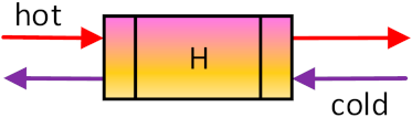
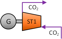
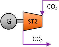
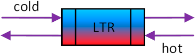
The thermal system used for data reconciliation calculation in this paper adopts the waste heat recovery system of a gas turbine proposed by Sun et al. [35], which uses an S-CO2 cycle with two S-CO2 turbines. The system layout diagram is shown in Figure 1. The S-CO2 bottom cycle consists of three heat exchangers, two S-CO2 turbines, one S-CO2 compressor, and one cooler. The technical data is listed in Table 1.
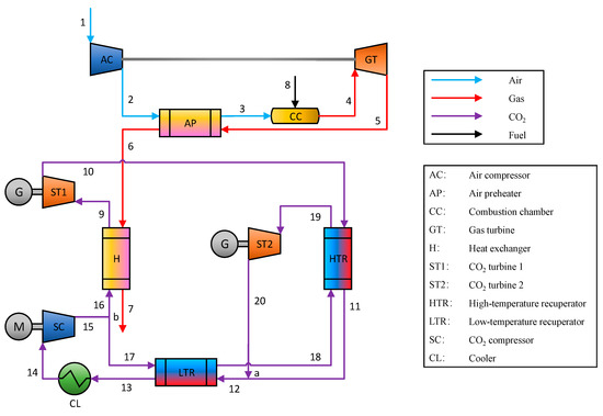
Figure 1.
Diagram of coupled system layout.

Table 1.
Different equipment characteristic parameters of waste heat recovery system.
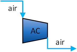
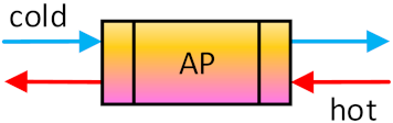
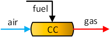
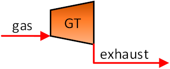
In the gas turbine cycle, after the air enters the cycle through stream 1, it first enters the air compressor and compressed. The compressed air enters the cold side of the air preheater to be heated by the gas turbine exhaust, then it enters the combustion chamber. In the combustion chamber, the fuel entering the circulation from stream 8 and preheated air are mixed for combustion, and the generated high-temperature gas makes the gas turbine generate power. After the work is done, the gas turbine exhaust enters the hot side of the air preheater for heating, then enters the heat exchanger to continue heating CO2. The heated exhaust of gas turbine is stream 7.
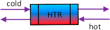
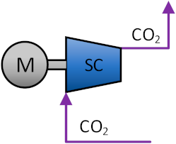
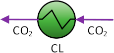
In the S-CO2 bottom cycle, the CO2 which is heated by the gas turbine exhaust enters the S-CO2 turbine 1 from stream 9 to do work. After the work is done, the CO2 successively enters a high-temperature recuperator and a low-temperature recuperator to heat another stream of CO2 from stream 17 to stream 19, then enters the cooler for cooling and enters the S-CO2 compressor for recompression. After being compressed by the S-CO2 compressor, the CO2 from stream 15 is divided into two streams. Stream 16 enters the heat exchanger to exchange heat with the gas turbine exhaust for continuous circulation. Stream 17 is heated by the two recuperators respectively, then enters the S-CO2 turbine 2 to generate power. After the work is done, it is merged with another stream of CO2 at stream 12 between the two recuperators. In this simple coupled circulation system, two S-CO2 turbines use heat exchangers to exchange heat with the gas turbine exhaust to generate electricity, which solves the recovery of gas turbine waste heat well.
In this paper, a gas turbine with exhaust temperature of 527.60 °C and exhaust mass flow of 92.90 kg/s was used for system construction and data reconciliation calculation. The following assumptions were made to simplify the calculation conditions:
- The waste heat recovery system is in a stable state, and the CO2 is always in a supercritical state;
- The external environment and the cooling water used by the cooler are both at 25 °C, 101 kPa;
- The pressure loss and heat loss of circulating equipment and pipelines can be ignored;
- The isentropic efficiencies of the air compressor and the S-CO2 compressor are constants, which are 80% and 85%, respectively;
- The isentropic efficiency of the gas turbine and the two S-CO2 turbines are also constants, which are all 90%.
3. Research Method
3.1. Heat Balance Model
The heat balance model of the waste heat recovery system is established according to the law of thermodynamics. For the system used in this paper, the following parameters are mostly concerned in the data reconciliation calculation process.
The total carbon dioxide mass flow in S-CO2 cycle expresses as follows:
where and are the mass flow of CO2 into ST1 and ST2 branches respectively.
The net output work of the coupled system expresses as follows:
where is the output power of the gas turbine, and are the output power of the S-CO2 turbines 1 and 2, respectively, and and are the consumption power of the air compressor and the S-CO2 compressor, respectively.
The heat balance equation models of the components in the system are shown in Table 2, where is the enthalpy value of stream , is the ideal enthalpy value after an isentropic process, is the mass flow of stream , is the heat exchange amount of a heat exchanger, and is the isentropic efficiency of the equipment.
Table 2.
Heat balance equations of each component.
3.2. Data Reconciliation Principle
In order to monitor the operating parameters in different position of the system, it is necessary to set sensors to obtain the measured values, and the data collected by these sensors is merged into the measurement data base as the input to data reconciliation. However, deviations in these measured values are unavoidable. Data reconciliation is a method to modify the measurement data under the premise of minimum total correction, so that all the measurement data can meet the constraint equations of the system. It can also solve the unknown data that is difficult to measure. When the whole thermal system is in a steady state, the vector composed of all known variables including characteristic data and measurement data with only random errors is defined as:
where is the true value vector of the known variable, and is the random error vector.
For the known variables in the thermal system, the problem that data reconciliation can solve is to minimize the sum of squares of the differences between the reconciliated values and the initial value under the constraint equations of energy and mass balance. Mathematically, this optimization problem can be converted to solving the least square solution that satisfies multiple constrained equations:
where is the component of known variable in Equation (3), is the reconciliated value of the known variable in group corresponding to (which compose the reconciled vector ), is the mean square deviation (standard deviation) corresponding to , is the object function of the optimization problem, is a equation vector representing a group of algebraic equations, and is the vector of the unknown variable.
If has a linear function to , then there is an analytical solution to this linear constrained problem after using the method of the unknown variable mentioned in Section 3.5. However, for general thermal systems, due to the existence of complex functions such as the property function of the working medium and the characteristic function of the equipment components, to should be nonlinear, so this problem is a quadratic solution problem with nonlinear constraints. The value of the unknown variable cannot be determined by the optimization problem and must be eliminated in the process of solving. In this paper, the improved Lagrange multiplier method proposed by VDI-2048 [36] is used for the calculation. This method converts constrained optimization into unconstrained optimization and nonlinear constraints into linear constraints in this problem in essence. After eliminating the effects of the unknown variable, the correction vector of the initial value vector is given as follows [36]:
where is the covariance matrix of the known variable vector, is the Jacobian matrix of equation vector to , is the inverse matrix of the covariance matrix of equation vector , which can be calculated as follows:
and presents the initial residual vector of whose notation in the upper right corner indicates that it has not been iterated. Here, the correction matrix of the covariance matrix is also given as follows:
which should be used to modify the covariance matrix .
The linearization method usually expands the nonlinear constrained equation according to Taylor’s formula and retains the first derivative term. However, in practical engineering applications, the expanded higher-order derivative term cannot be simply ignored by Jacobian matrix linearization, and the residual of constraint equation cannot be eliminated by a simple correction. Thus, the data reconciliation model established in this paper adopts the iterative algorithm framework developed by You et al. [37]. The correction vector iteration format is constructed as follows:
where is the number of iterations. Before the iterative computation begins, the updated Jacobian matrix is recalculated by numerical differentiation, and the covariance matrix of the equation residual vector is recalculated by Equation (6), then the iterative process continues. The covariance matrix of the correction vector for the iterative calculation process can be solved as follows:
And the iterative process is terminated when the incremental norm of the correction vector is too small:
where is the convergence limit. In this way, the optimizing calculation of data reconciliation for the initial value of variables is completed.
3.3. Gross Error Identification
Under normal circumstances, data reconciliation has a good coordination and optimization effect for random errors obeying statistical distribution law, but it may have a poor effect for gross errors disobeying statistical distribution law. The reason is that gross errors will be dispersed to all related data in the system during the process of data reconciliation, which may lead to a greater degree of overall deviation in the reconciliated data.
Gross error identification usually adopts the statistical hypothesis test method, which is only based on the operation data, has the characteristics of strong applicability, economy and simple operation, and has been widely studied and applied. Different test statistics correspond to the hypothesis statistical test methods, which commonly include the global test method, the constraint equation test method and the measurement test method. The data reconciliation model established in this paper adopts the global test method and the measurement test method.
The global test method is a method to judge whether a gross error in the whole system calculation model exists. In the global test method, the global test statistic can be defined as follows [38]:
If the gross error does not exist in the whole system, the test statistic following the chi-square distribution should meet the following requirements:
where is the chi-square distribution critical value. Normalization of this formula which is easy to use results in the following [38]:
where means quality factor is used to characterize the gross error of the whole system.
Even if the whole system satisfies Equation (15), there may still be gross errors in some parameters, and the measurement test method is used to identify the gross errors of parameters. In the measurement test method, in order to realize the identification of suspicious data with gross errors, the test statistics of variable based on the correction vector can be constructed as follows [36]:
where is the correction value of variable . For the right side of Equation (16), when reaches the allowable error maximum , there is the following equation:
where is the lower fraction of the normal distribution, which can be obtained by looking up the statistics table. In the process of systematic data reconciliation calculation, given which means the confidence level is 95%, it can be seen from the table that . Under normal circumstances, this should be:
This means that there are no anomalies in this set of data. If Equation (18) is not satisfied, it means that the confidence probability of the reconciliated value is less than 5%, and it can be considered that the parameter is suspicious with gross error. At this time, it is reasonable to think that an instrument error or equipment breakdown may have occurred, and further inspection must be carried out.
Therefore, how do we use practical identification methodology in data reconciliation process? First, we can build the overall model of heat balance equations and redundant constraint equations after determining known and unknown variables. At this time, we can give the global test statistic of the model and the test statistics of each variable respectively according to above formulas, which can be used as criteria for testing gross errors. Later, as the calculation of iterative process gradually converges, can be used to test whether the reconciliated system model has gross errors and can be used to test whether the reconciliated single variable contains gross errors.
3.4. Sensor Arrangement
The variables in the system can be divided into the known variables and the unknown variables. The known variables used as input for data reconciliation include two types: characteristic data and measurement data.
Characteristic data are generally based on characteristic parameters of the equipment or design values of system operation because of their relative stability in most situation. The characteristic data used in this paper are shown in Table 1.
For the measurement data, it is necessary to arrange sensors in each part of the whole system. There are three types of sensors: pressure, temperature and mass flow. The arrangement of sensors in this paper is shown in Table 3. It can be seen that three types of sensors are mainly arranged around the S-CO2 bottom cycle, while some sensors in the gas turbine cycle mainly supplement some necessary data and provide little redundancy for data reconciliation. There are more temperature sensors than sensors for pressure and mass flow, and several temperature sensors are arranged in one stream of waste heat recovery system in some cases.
Table 3.
Arrangement of sensors in different stream of waste heat recovery system.
The measurement uncertainty represents the reasonable distribution of the measured value under a specific probability. It can quantify the possible deviation of the measured value. It should be noted that the uncertainty here is not equivalent to the uncertainty level of the measurement instrument, but is only used in data reconciliation calculations. It is similar to a weight coefficient, reflecting the uncertainty of the data before and after the reconciliation.
For each pressure, temperature and mass flow sensor, there is a certain uncertainty. Even small fluctuations in environmental conditions will affect the measurement performance and lead to deviations. In general, the measurement uncertainty can be empirically assumed as either the instrument accuracy or the maximum permissible deviation in practice [28]. In this paper, the specific assumptions of uncertainty are as follows: the absolute uncertainty is taken as 2 °C for temperature sensors and parameters, the relative uncertainty is taken as 2% for pressure sensors and parameters, the relative uncertainty is taken as 5% for the mass flow sensors and parameters and the relative uncertainty is taken as 10% for the characteristic parameters such as ratio and efficiency.
3.5. Unknown Variables and Redundant Equations
For unknown variables in the system, because the value of unknown variables cannot be determined by the optimization problem, it is necessary to eliminate their influence through a reasonable method. The solution process needs to be added after the introduction of the unknown variables. In view of this, this paper adopts the “Intermediate variable method” [37]. By establishing the thermal balance model of the system, the unknown variable is expressed through the known variable and the uncertainty is also derived, so that the unknown variable can be better obtained in the reconciliation process. This method does not need to specify the initial value, and directly establishes the relationship between the known variables in the previous section and the residual vector of the equation. This method of eliminating unknown variables can make the convergence performance of the system more stable.
For example, for the HTR, our known variable is its terminal temperature difference, but we do not know the inlet or outlet temperature of the CO2 stream on both sides. Then, in the data reconciliation process, these temperature parameters are defined as unknown variables, which need to be expressed by the heat balance of other known variables in the system. After that, these unknown variables and all known variables participate in the data reconciliation process of the model.
After the heat balance model is established, the role of several heat balance equations is to solve the above unknown data using the measured or designed values of some sensors. The heat balance equations used are independent from the equations involved in the optimization problem, and cannot be reused for the subsequent iterative solution of the residual vector of the equation. Among the remaining sensors, there are multiple sensors in the same stream or sensors with known equipment characteristic parameters. These sensors can be involved in the redundant constraint equations as well, which are used to solve the subsequent optimization problem.
4. Model Verification
According to the above principles, we write a computer program of data reconciliation with Python 3.9.0 language, introduced REFPROP physical property library to calculate, so that we can establish heat balance model and data reconciliation model respectively.
The model established in this paper is verified by using the system model established by Sun et al. [35]. The specific verification results are shown in Table 4, in which the parameters used for comparison in this paper are the parameters of the design working condition after heat balance calculation under the same initial conditions. It can be seen from the table that the thermodynamic model established in this paper is in good agreement and has high credibility with the model of Sun L’s work.
Table 4.
Comparison of model validation.
Since the design value parameters of the system under design conditions strictly meet the constraint of energy and mass balance, theoretically there should be no coordination and correction process for data reconciliation calculation using the design value as the initial measured value without adding random errors. To verify the reliability of the data reconciliation algorithm, the data reconciliation calculation results of the model established in this paper are shown in Table 5. The reconciliated value and the design value have a good consistency, which proves that our model is dependable.
Table 5.
Verification results of data reconciliation model under the design condition.
5. Results and Discussion
5.1. General Computing Overview
The data reconciliation model used in this paper is based on design values of the system. The known variables of data reconciliation are given by adding certain random errors to the characteristic data and measurement data under the design condition, and the subsequent iterative calculation process of data reconciliation is carried out. The known variables with random errors can be represented here as follows:
where is the design value corresponding to the known variable and is the coefficient of random errors. Here, for the random error coefficient, the uniform distribution in [−1, 1] is taken to enhance the convergence of the data reconciliation calculation process. For gross errors, it is necessary to add a gross error much larger than on the basis of the corresponding design value of the known variable.
The data reconciliation model in this paper calculates ten groups of working conditions. Among them, the first two working conditions do not contain gross errors, and the last eight working conditions all contain one to four gross errors. The specific working conditions are set as shown in Table 6. Among them, Conditions 1 and 2 only contain automatically generated random errors, the purpose of which is to study the reconciliation ability and effect of the data reconciliation model without gross errors. Condition 3 to Condition 6 add one gross error of temperature, pressure or mass flow sensor, respectively, and Condition 7 to Condition 10 add two to four gross errors, respectively, to study the model ability of identifying suspicious sensors with gross errors and reconciliating of the overall system parameters under the condition of gross errors.
Table 6.
Setting of sensors with gross errors under different working conditions.
Under the above ten working conditions, the quality factors of the system in the data reconciliation calculation process which is defined in Equation (15) are shown in Figure 2. The quality factors of ten working conditions are all less than 1, which meets the requirements of global gross error inspection. Quality factor is a test statistic that characterizes whether there are serious errors within the whole system [37]. Only when it is less than 1 it can be indicated that it has passed the global inspection, which means the calculation of the system model does not contain serious errors at the system level. In addition, the quality factors of Conditions 1 and 2 which do not include gross errors are about 0.2. It can also be seen in subsequent working conditions that with the addition and setting of sensors with gross errors, the quality factor is gradually increased. Especially when adding four gross errors in Condition 10, its quality factor has been as high as 0.6 or so.
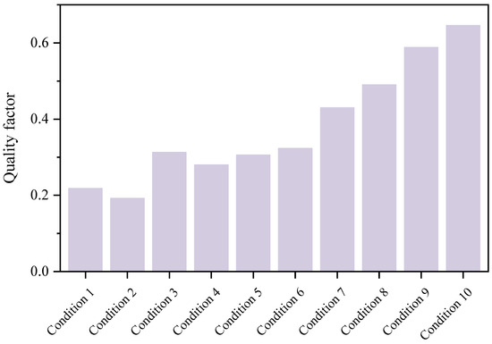
Figure 2.
Quality factor of parameters under different working conditions.
As we mentioned earlier, the established data reconciliation model requires an iterative process, and its convergence criteria are determined by the residual of redundant equations. Since there are many redundant equations, the residual of equations is introduced here as the determination of iterative convergence, which is calculated as follows [37]:
where represents the number of equations. It is only used to judge the iteration in the whole reconciliation calculation process, and has no physical significance. The iteration of residual of redundant equations under ten working conditions is shown in Figure 3. The iterative calculation of data reconciliation can converge within three steps, and the residual of redundant equations has been reduced to the magnitude order of 10−4 or below, which indicates that the data reconciliation model has a good convergence for the reconciliation process of system parameters, and has a good effect in reducing the residual of the redundant equations.
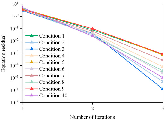
Figure 3.
Iterative calculation of equation residual under different working conditions.
5.2. Data Reconciliation Without Gross Errors
This section is an overview of two calculation conditions that do not include gross errors. The reconciliation results of some parameters under Conditions 1 and 2 are shown in Table 7 and Table 8, where Val. represents value, De. represents deviation, and Un. represents uncertainty. As can be seen from the tables, since Conditions 1 and 2 do not have gross error sensors, the overall reconciliation effect of the system is relatively good, and the overall reconciliation trend of the two is consistent. The level of reconciliated deviation is small. It can be seen deviations of most parameters under two working conditions are less than 1, and the deviations of very few parameters are also fluctuating around 1%. Measured values of known variables or calculated values of unknown variables still have large deviations from the design values within the allowable deviation range even if they do not contain gross errors. Most of them are mass flow sensors such as mass flow of gas and mass flow of CO2 in ST1, etc. The deviations of these sensors have been significantly reduced after reconciliation. However, in fact, the deviations of a very small number of parameters are increased, such as SC output pressure under Condition 1 and AC power under Condition 2. This is because data reconciliation is a reconciliation process for parameters of the whole thermal system, and its essence is to disperse the large deviations of some parameters into other parameters to improve the quality of all parameters. In addition, compared with the change of uncertainty before and after reconciliation, the uncertainties of parameters also have a very obvious decline, and those after reconciliation are below 3%. It can be shown that the data reconciliation greatly reduces the uncertainty of the parameter whether known variables or unknown variables, and effectively improve the accuracy of measurement data.
Table 7.
Reconciliation results of some parameters in Condition 1.
Table 8.
Reconciliation results of some parameters in Condition 2.
The distribution of standard deviation in Conditions 1 and 2 are shown in Figure 4 and Figure 5. The data reconciliation has a good effect on the deviation aggregation of parameters of such a thermal system, and the overall distribution curve of the deviation in Conditions 1 and 2 after reconciliation has an obvious effect of concentration towards the origin than that before reconciliation.
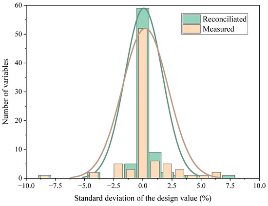
Figure 4.
Distribution of standard deviation in Condition 1.
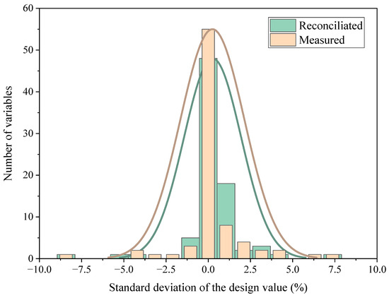
Figure 5.
Distribution of standard deviation in Condition 2.
The distribution of uncertainty in Conditions 1 and 2 are shown in Figure 6 and Figure 7. The uncertainty distributions of the two are basically the same, which indicates that the data reconciliation has a good correction for random errors and always converges on the data results with higher precision. At the same time, similar to the deviation distribution, the distribution curve of the uncertainty after reconciliation also has an obvious effect on the origin concentration before reconciliation, which also explains the improvement of the overall data accuracy.

Figure 6.
Distribution of uncertainty in Condition 1.
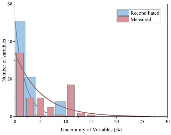
Figure 7.
Distribution of uncertainty in Condition 2.
5.3. Data Reconciliation with Gross Errors
This section is an overview of eight calculation conditions with gross errors. For each working condition, the recognition of sensors with gross errors is shown in Table 9. On the basis of passing the global inspection, the sensors with gross errors under each working condition are well identified, which is based on Equation (16) because the calculated criterion value of is greater than 1.96. Compared with the gross errors setting in Table 6, it is found that the two have a good consistency, which also indicates that the data reconciliation model established in this paper is relatively effective in identifying the gross errors of some sensors in the thermal system.
Table 9.
Identification with gross errors of the working conditions.
The reconciliation results of other sensors in Condition 10 except the sensors with gross errors is shown in Table 10. The deviation of sensors with gross errors is dispersed among all parameters, resulting in an increase in the deviation of some parameters from the design value standard, but the overall deviation level is still low. The highest deviation appears in unknown variables of power and fluctuates around 2%. This result can also show that the gross errors have an obvious influence on the data reconciliation effect, because these errors will not be eliminated, but only dispersed. Even so, it can be seen from the change of uncertainty that the data reconciliation still improves the data accuracy significantly in this case.
Table 10.
Reconciliation results of some parameters in Condition 10.
The distribution of standard deviation in Condition 10 is shown in Figure 8. Due to the addition of gross errors and more random errors, the overall distribution curve has a wider range. However, after data reconciliation, all deviations can be concentrated to the origin. Although the number of variable deviations near the origin is less than before reconciliation due to the effect of large error dispersion, the quality of parameters has been significantly improved. If the gross errors identified can be eliminated in the process of practical application, the reconciliation effect will be better.
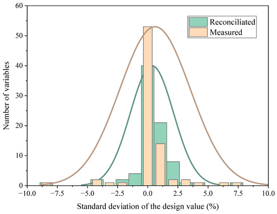
Figure 8.
Distribution of standard deviation in Condition 10.
The uncertainty distribution of working condition 10 is shown in Figure 9. There is no significant difference between the distribution trend of uncertainty after adding coarse errors and the previous working conditions. After coordination, the degree of uncertainty reduction is more obvious, the homogeneity is concentrated at the origin and the accuracy of measurement data is improved.
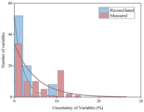
Figure 9.
Distribution of uncertainty in Condition 10.
6. Conclusions
In this paper, a data reconciliation model is established based on a waste heat recovery system of a gas turbine using an S-CO2 cycle with two S-CO2 turbines. The thermal system and the data reconciliation model are well fitted with the reference values. The data reconciliation calculation shows that the overall deviation level of each parameter of the thermal system after reconciliation is obviously reduced, and the uncertainty is also reduced, which reflects that the data reconciliation technology can improve the measurement accuracy of thermal system. In the case of adding random errors, the measurement deviation of key parameters in the system, such as the total mass flow of CO2, can be reduced to less than 1%. The power values, such as ST and SC, can be obtained with high data accuracy, and the deviation is also about 1%. In the conditions of adding gross errors, all kinds of sensors containing gross errors can be well identified and eliminated through the data reconciliation model, and the accuracy of the overall measurement data is still improved to a certain extent even under the influence of gross errors.
In summary, the data reconciliation model established in this paper can provide a certain reference for the accuracy of thermal system parameter measurement, and can be applied to scenarios such as parameter correction of thermal system test bench and equipment error detection, which has deep research significance. Building a system test bench can be used to validate the concrete results of the data reconciliation method and bring them into real-world environments. At the same time, it may be necessary to increase the research topics, such as variable operating conditions and heat transfer efficiency, to ensure the rigor of the test. In addition, further exploration of the performance in data reconciliation model in actual advanced power cycle is needed.
Author Contributions
Conceptualization, L.X. and J.Y.; Methodology, L.X. and J.Y.; Validation, J.Y., J.W. and Y.L.; Formal analysis, L.X.; Investigation, J.W., Y.L. and D.Z.; Writing—original draft, L.X.; Writing—review and editing, L.X., J.Y., J.W., Y.L. and D.Z.; Supervision, D.Z. All authors have read and agreed to the published version of the manuscript.
Funding
The work was fully supported by the University Joint Program of Shaanxi Province Key Research Project—Major Project (2022GXLH-01-17) and the Major Project of Shaanxi Province Key Research Project (2024PT-ZCK-47).
Institutional Review Board Statement
Not applicable.
Informed Consent Statement
Not applicable.
Data Availability Statement
Data will be made available on request.
Conflicts of Interest
The authors declare no conflicts of interest.
Nomenclature
| Symbol | Meaning |
| AC | Air compressor |
| AP | Air preheater |
| CC | Combustion chamber |
| CL | Cooler |
| GT | Gas turbine |
| H | Heat exchanger |
| HTR | High-temperature recuperator |
| LTR | Low-temperature recuperator |
| SC | S-CO2 compressor |
| ST1 | S-CO2 turbine 1 |
| ST2 | S-CO2 turbine 2 |
| Enthalpy | |
| Mass flow | |
| Heat exchange amount | |
| Power | |
| Efficiency | |
| The equation vector representing a set of algebraic equations | |
| The initial residual vector of the equation vector | |
| The initial residual vector after iterations | |
| The Jacobian matrix of equation vector versus | |
| The test statistics of variable based on the correction vector | |
| The covariance matrix of the equation vector | |
| The covariance matrix of the known variable vector | |
| The vector of the unknown variable. | |
| The component of | |
| The reconciliated value of the known variable | |
| The vector composed of all known variables | |
| The reconciliated value vector of the known variable | |
| The true value vector of the known variable | |
| The lower fraction of the normal distribution | |
| The random error vector | |
| The convergence limit | |
| The correction vector of the initial value vector | |
| The correction value | |
| The correction vector of the initial value vector after iterations | |
| The maximum allowable error | |
| The mean square deviation (standard deviation) | |
| The coefficient of random errors |
References
- Tian, H.; Ding, H.; Bin, W. A Summary of wearable textiles power generation. In IOP Conference Series: Earth and Environmental Science; IOP Publishing: Bristol, UK, 2021; Volume 772, p. 012037. [Google Scholar]
- EI Statistical Review of World Energy 2024; Energy Institute: London, UK, 2024.
- Heppenstall, T. Advanced gas turbine cycles for power generation: A critical review. Appl. Therm. Eng. 1998, 18, 837–846. [Google Scholar] [CrossRef]
- Can Gülen, S. Étude on gas turbine combined cycle power plant—Next 20 years. J. Eng. Gas Turbines Power 2016, 138, 051701. [Google Scholar] [CrossRef]
- Zhang, C.; Shu, G.; Tian, H.; Wei, H.; Liang, X. Comparative study of alternative ORC-based combined power systems to exploit high temperature waste heat. Energy Convers. Manag. 2015, 89, 541–554. [Google Scholar] [CrossRef]
- Rajinesh, S.; Miller, S.A.; Rowlands, A.S.; Jacobs, P.A. Dynamic characteristics of a direct-heated supercritical carbon-dioxide Brayton cycle in a solar thermal power plant. Energy 2013, 50, 194–204. [Google Scholar]
- Ruby Meena, A.; Senthil Kumar, S. Genetically tuned fuzzy PID controller in two area reheat thermal power system. Russ. Electr. Eng. 2016, 87, 579–587. [Google Scholar] [CrossRef]
- Chowdhury, J.I.; Thornhill, D.; Soulatiantork, P.; Hu, Y.; Balta-Ozkan, N.; Varga, L.; Nguyen, B.K. Control of supercritical organic Rankine cycle based waste heat recovery system using conventional and fuzzy self-tuned PID controllers. Int. J. Control Autom. Syst. 2019, 17, 2969–2981. [Google Scholar] [CrossRef]
- Christoph, S.; Dimache, L.; Lohan, J. Operational Optimisation of a Heat Pump System with Sensible Thermal Energy Storage using Genetic Algorithm: A Case Study. Therm. Sci. 2018, 22, 2189–2202. [Google Scholar]
- Qian, Y.; Du, W.-J.; Cheng, L. Optimization design of heat recovery systems on rotary kilns using genetic algorithms. Appl. Energy 2017, 202, 153–168. [Google Scholar]
- Reza, B.; Eiamsa-ard, S. Genetic algorithm multiobjective optimization of a thermal system with three heat transfer enhancement characteristics. J. Enhanc. Heat Transf. 2020, 27, 123–141. [Google Scholar]
- Lin, Y.; Wang, H.; Hu, P.; Yang, W.; Hu, Q.; Zhu, N.; Lei, F. A study on the optimal air, load and source side temperature combination for a variable air and water volume ground source heat pump system. Appl. Therm. Eng. 2020, 178, 115595. [Google Scholar] [CrossRef]
- Shankar, N.; Jordache, C. Data Reconciliation and Gross Error Detection: An Intelligent Use of Process Data; Elsevier: Amsterdam, The Netherlands, 1999. [Google Scholar]
- Romagnoli, J.A.; Sánchez, M.C. Data Processing and Reconciliation for Chemical Process Operations; Elsevier: Amsterdam, The Netherlands, 1999. [Google Scholar]
- Kretsovalis, A.; Mah, R.S.H. Observability and redundancy classification in multicomponent process networks. AIChE J. 1987, 33, 70–82. [Google Scholar] [CrossRef]
- Crowe, C.M.; Campos, Y.G.; Hrymak, A. Reconciliation of process flow rates by matrix projection. Part I: Linear case. AIChE J. 1983, 29, 881–888. [Google Scholar] [CrossRef]
- Crowe, C.M. Reconciliation of process flow rates by matrix projection. Part II: The nonlinear case. AIChE J. 1986, 32, 616–623. [Google Scholar] [CrossRef]
- Swartz, C.L.E. Data reconciliation for generalized flowsheet applications. In Proceedings of the ACS National Meeting, Dallas, TX, USA, 9–14 April 1989. [Google Scholar]
- Reilly, P.M.; Carpani, R.E. Application of statistical theory of adjustment to material balances. In Proceedings of the 13th Canadian Chemical Engineering Congress, Montreal, QC, Canada, 23 October 1963. [Google Scholar]
- Mah, R.S.H.; Tamhane, A.C. Detection of gross errors in process data. AIChE J. 1982, 28, 828–830. [Google Scholar] [CrossRef]
- Narasimhan, S.; Mah, R.S. Generalized likelihood ratio method for gross error identification. AIChE J. 1987, 33, 1514–1521. [Google Scholar] [CrossRef]
- Narasimhan, S.; Mah, R.S. Generalized likelihood ratios for gross error identification in dynamic processes. AIChE J. 1988, 34, 1321–1331. [Google Scholar] [CrossRef]
- Holly, W.; Cook, R.; Crowe, C.M. Reconciliation of mass flow rate measurements in a chemical extraction plant. Can. J. Chem. Eng. 1989, 67, 595–601. [Google Scholar] [CrossRef]
- Sriniketh, S.; Billeter, J.; Narasimhan, S.; Bonvin, D. Data reconciliation for chemical reaction systems using vessel extents and shape constraints. Comput. Chem. Eng. 2017, 101, 44–58. [Google Scholar]
- Humaad, I.; Ati, U.M.K.; Mahalec, V. Heat exchanger network simulation, data reconciliation & optimization. Appl. Therm. Eng. 2013, 52, 328–335. [Google Scholar]
- Martínez-Maradiaga, D.; Bruno, J.C.; Coronas, A. Steady-state data reconciliation for absorption refrigeration systems. Appl. Therm. Eng. 2013, 51, 1170–1180. [Google Scholar] [CrossRef]
- Magnus, L.; Jansky, J. Process data reconciliation in nuclear power plants. In Proceedings of the EPRI Nuclear Power Performance Improvement Seminar, Saratoga Springs, NY, USA, 15–16 July 2002. [Google Scholar]
- Magnus, L. Power recapture and power uprate in NPPS with process data reconciliation in accordance with VDI 2048. Int. Conf. Nucl. Eng. 2006, 42428, 7–14. [Google Scholar]
- Svein, S.; Berg, Ö. Data reconciliation and fault detection by means of plant-wide mass and energy balances. Prog. Nucl. Energy 2003, 43, 97–104. [Google Scholar]
- Damianik, V.E.; Schirru, R. Simultaneous model selection, robust data reconciliation and outlier detection with swarm intelligence in a thermal reactor power calculation. Ann. Nucl. Energy 2011, 38, 1820–1832. [Google Scholar]
- Hartner, P.; Petek, J.; Pechtl, P.; Hamilton, P. Model-based data reconciliation to improve accuracy and reliability of performance evaluation of thermal power plants. Turbo Expo Power Land Sea Air 2005, 47276, 195–200. [Google Scholar]
- Jiang, X.; Liu, P.; Li, Z. Data reconciliation and gross error detection for operational data in power plants. Energy 2014, 75, 14–23. [Google Scholar] [CrossRef]
- Chen, P.-C.; Andersen, H. The implementation of the data validation process in a gas turbine performance monitoring system. Turbo Expo Power Land Sea Air 2005, 46997, 609–616. [Google Scholar]
- Can, G.S.; Smith, R.W. A simple mathematical approach to data reconciliation in a single-shaft combined cycle system. J. Eng. Gas Turbines Power. Mar 2009, 131, 021601. [Google Scholar]
- Sun, L.; Wang, D.; Xie, Y. Energy, exergy and exergoeconomic analysis of two supercritical CO2 cycles for waste heat recovery of gas turbine. Appl. Therm. Eng. 2021, 196, 117337. [Google Scholar] [CrossRef]
- VDI-2048: Control and Quality Improvement of Process Data and Their Uncertainties by Means of Correction Calculation for Operation and Acceptance Tests; Association of German Engineers; VDI Verein Deutscher Ingenieure: Düsseldorf, Germany, 2017.
- You, J.; Wu, J.; Xu, L.; Xie, Y.; Qiu, J.; Wan, L.; Qin, Q. Exploration on the comprehensive data reconciliation framework for unknown parameter inference in the nuclear power plant system. Appl. Therm. Eng. 2024, 247, 123138. [Google Scholar] [CrossRef]
- Langenstein, M.; Jansky, J.; Laipple, B.; Eitschberger, H.; Grauf, E.; Schalk, H. Finding megawatts in nuclear power plants with process data reconciliation. Int. Conf. Nucl. Eng. 2004, 46881, 43–52. [Google Scholar]
Disclaimer/Publisher’s Note: The statements, opinions and data contained in all publications are solely those of the individual author(s) and contributor(s) and not of MDPI and/or the editor(s). MDPI and/or the editor(s) disclaim responsibility for any injury to people or property resulting from any ideas, methods, instructions or products referred to in the content. |
© 2024 by the authors. Licensee MDPI, Basel, Switzerland. This article is an open access article distributed under the terms and conditions of the Creative Commons Attribution (CC BY) license (https://creativecommons.org/licenses/by/4.0/).