Energy Management Strategies for Extended-Range Electric Vehicles with Real Driving Emission Constraints

Abstract

Fuel economy has long been the core control objective in the energy management strategies of extended-range electric vehicles (EREVs), but little research has considered real driving emissions. In this paper, the real driving emissions of an EREV are investigated, and the abnormal pollutant emissions caused by engine start–stop events are clarified. Accordingly, an interpolated-startup-corrected method is proposed to construct real driving emission models. Next, an optimization problem is constituted with real driving emissions as the constraints and fuel consumption as the objective. The optimization problem is solved using a dynamic programming (DP) algorithm embodying the interpolated-startup-corrected emission models, and the start–stop reduction strategies and condition migration strategies are derived. Compared to the strategy without the emission constraints, the CO and NO_x emissions under the no-start–stop strategy are cut down by about 70%; the PN emissions are even orders of magnitude lower. Meanwhile, the condition migration strategy can compromise the fuel economy and pollutant emissions by adjusting the engine operating points, thus possibly limiting pollutant emissions beyond the start–stop reduction strategy.

1. Introduction

Energy shortage [1], environmental pollution [2], and global warming [3] are urgent problems that need to be solved for the development of society today. As a significant contributor to the overconsumption of fossil fuels, road transport has been widely criticized [4], which spurs transport electrification and gives rise to electrified vehicles, such as battery electric vehicles (BEVs), hybrid electric vehicles (HEVs), plug-in electric vehicles (PHEVs), and extended-range electric vehicles (EREVs) [5,6,7]. An EREV uses a generator in series with an internal combustion engine so that when the state of charge (SOC) of the battery falls below a specified level, the engine starts and continues the vehicle’s journey by recharging the battery [8,9], thus solving the problem of range anxiety [10]. In addition, the engine converts heat from fuel combustion into mechanical energy, which is then converted by a generator into electrical energy that is either stored in the battery or fed directly to an electric motor to drive the vehicle [11]. During this process, engine speed is decoupled from vehicle travel speed. As a result, the engine can achieve high thermodynamic efficiency by operating in its optimal operating region [12]. Much research has been carried out to design energy management strategies to coordinate the power allocation between the engine and the electric motor [13,14]. These developed energy management strategies include rule-based strategies and optimization-based strategies [15,16]. Rule-based strategies are usually basic control logic extracted from knowledge and experience, and these strategies are empirically adjusted using data acquired offline [17]. Optimization-based strategies, such as model predictive control [18,19], dynamic programming (DP) [20,21], and deep reinforcement learning (DRL) [22,23], employ control action as a solution to the optimization problem.

Fuel economy has long been the core control objective in EREV energy management strategies [24,25,26]. However, in pursuit of efficient operation, the engine must frequently switch between efficient and shutdown conditions [27]. Engine speed rapidly increases from zero to thousands of revolutions per minute in one second during the start-up process. This extreme transient change in the engine’s frequent start–stop operating conditions results in abnormal exhaust emissions, so the tailpipe after-treatment system must be reconfigured [28]. Inevitably, the superior fuel economy of EREVs is usually accompanied by a significant increase in exhaust pollutant emissions. Currently, only a few works touch on pollutant emissions for EREV energy management strategies. Liu et al. [29] proposed a hybrid-point-line energy management strategy based on multi-objective optimization for EREVs and then applied barebones multi-objective particle swarm optimization to solve a multi-objective optimization model that takes into account energy consumption, emissions, and battery life. In their study, the establishment of the engine fuel efficiency map and the comprehensive emission (CO, HC, and NO_x) map are all derived from actual engine steady-state measurements. Lin et al. [30] developed a multi-objective optimization adaptive control strategy based on an equivalent consumption minimization strategy and an adaptive equivalence factor method. The strategy models the relationship between road grade and emissions and uses a proportional-integral controller to update the equivalence factor based on road grade. However, the emission model is still based on engine steady-state performance test data. Chang et al. [31] proposed an adaptive two-point energy management strategy to improve vehicle economy, reduce emissions, and extend battery life. This article examines gas pollutant emissions through engine steady-state bench tests to study the relationship between EREV exhaust emissions and engine operating conditions. Tang et al. [32] proposed three distributed DRL-based energy and emission management strategies to achieve near-optimal fuel economy and outstanding computational efficiency, regarding a DP strategy as the optimal benchmark. In the DRL-based strategies, the engine’s fuel consumption and emission model are still modeled by steady-state engine performance maps. As can be seen, these existing studies tried to use steady-state engine performance data measured on a laboratory engine bench to construct emission models. However, under real driving conditions, the engine operating state and control parameters change instantaneously, and transient pollutant emissions differ from those under stable engine operating conditions on the test bench [33]. Many existing studies have revealed that the dynamic characteristics of the engine’s operating conditions influence exhaust pollutant emissions [34]. On-road driving tests have also verified that the real driving pollutant emissions in the aggressive driving style are significantly higher than those under the smooth driving style [35,36,37]. Evidently, emission models based on steady-state engine performance test data are much less likely to characterize the severe emissions resulting from extreme transient changes of engine states in the engine’s start-up, making it challenging to consider exhaust emissions in energy management strategies for EREV.

This study aims to develop a dynamic model of engine pollutant emissions to fully reflect the emission deterioration caused by engine start–stop during real driving conditions of EREVs and to optimize energy management strategies with strict constraints on pollutant emissions. This study investigates the real driving emissions of an EREV based on regulatory test procedures and determines the engine start-up events that lead to abnormal pollutant emissions under real driving conditions. Inspired by real driving emission characteristics, an interpolated-startup-corrected method is proposed to construct the real driving emission model of EREV, which approximates the engine non-start-up conditions to the steady operating conditions and corrects the engine start-up emissions. Then, an optimization problem is constructed with real driving emissions as the constraints and minimum fuel consumption as the objective. Using the penalty function method, the emission constraints are assembled with the objective function to guide the optimization solution toward satisfying the emission constraints. Next, the DP algorithm embodying the interpolated-startup-corrected emission models is developed by inventing multiple interpolation operations in the value-space and action-space domains, which is used to solve the optimal engine operating sequence to obtain the lowest fuel consumption under the given emission limits. This study creates a new pathway to combine fuel economy-centered strategies and emission pollution-limited strategies for the energy management of EREVs.

This paper is organized as follows: Section 2 introduces the EREV real driving emission tests based on the regulatory test procedures, demonstrates the modeling methodology and model validation of the interpolation-startup-correction emission model, and proposes the DP algorithm embedding the real driving emission model for energy management strategy optimization. The start–stop reduction strategies and condition migration strategies resulting from the DP algorithm are analyzed, explained, and discussed in Section 3. Finally, conclusions are drawn in Section 4.

2. Models and Methods

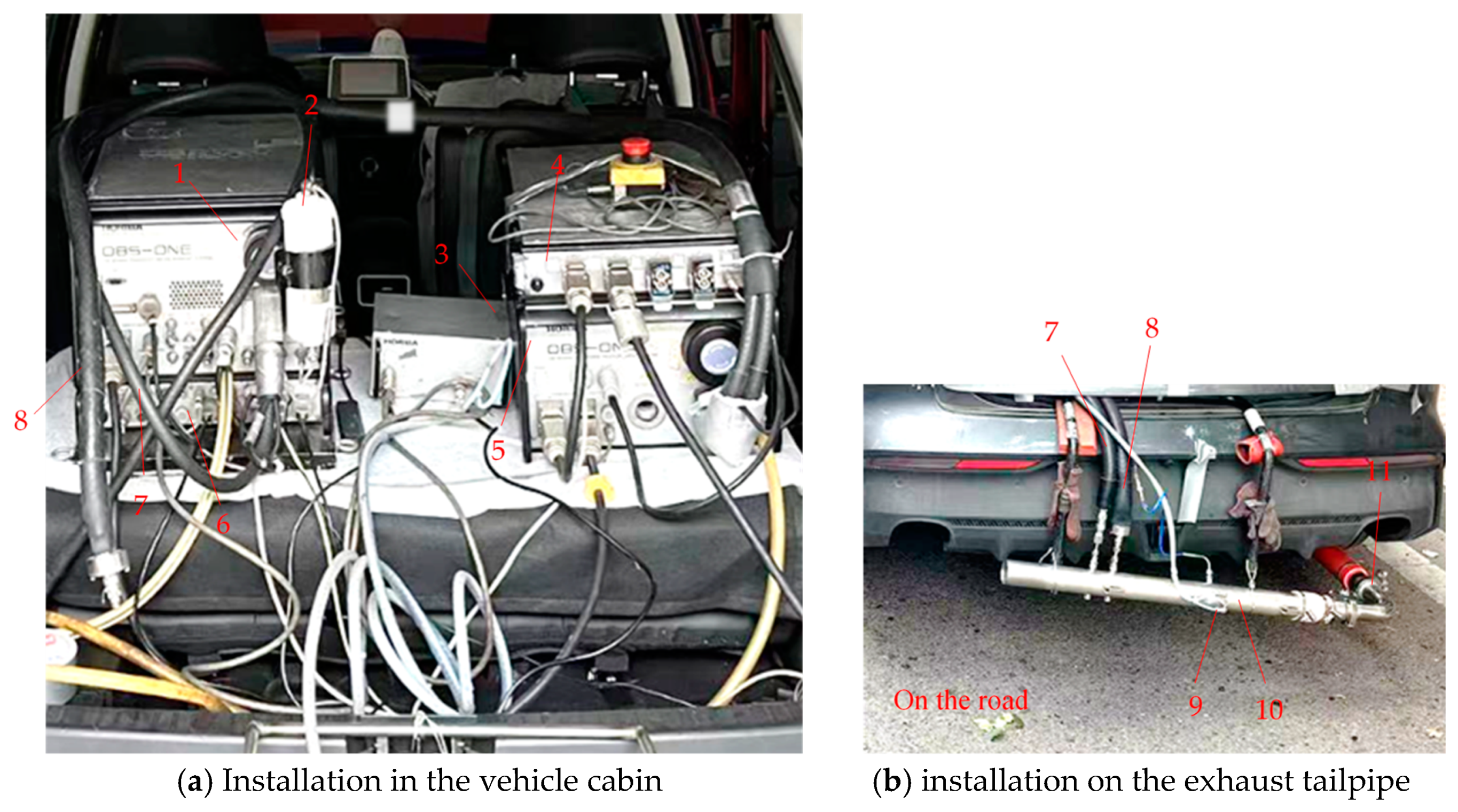
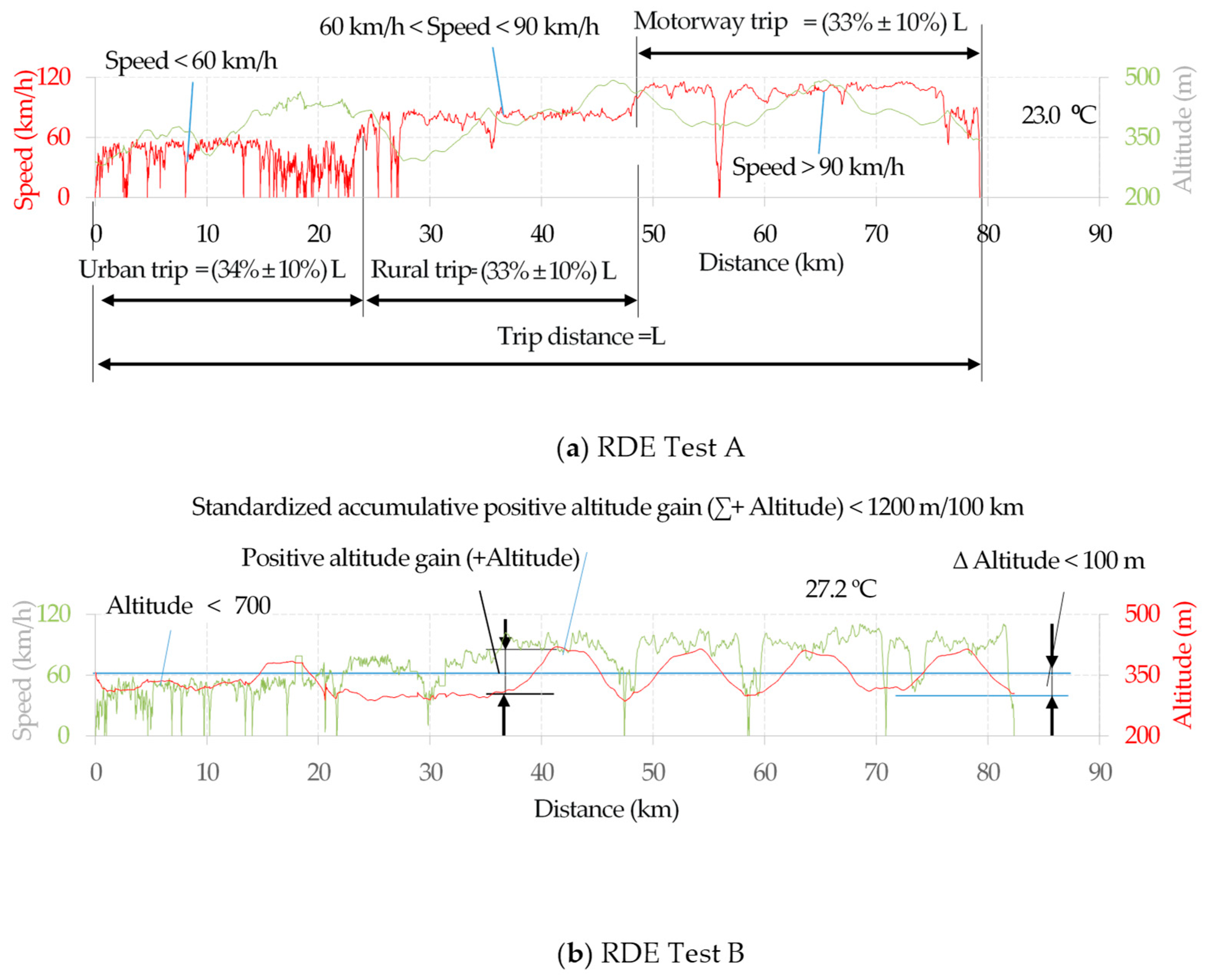
2.1. Real Driving Emission Tests

Vehicle pollutant emissions have been widely measured using the driving cycle testing method in a laboratory environment. The driving cycle testing method combines some common vehicle operating conditions and severe polluting emission conditions into a test cycle, and the specific-distance pollutant emissions of the vehicle are measured during this test cycle on a laboratory chassis dynamometer. However, the vehicle’s real driving conditions are very diverse. The constructed test cycles (e.g., NEDC, WLTC) cannot adequately characterize the real driving conditions of the vehicles, resulting in the emission test results of the driving cycle test method being often inconsistent with the reality of vehicle emissions [38,39,40,41]. Thus, Europe introduced the real driving emission test procedure in the Euro 6 emission standards, which requires real-time measurement of pollutant emissions under on-road driving conditions using a portable emission measurement system (PEMS). It has become a global consensus to examine vehicle pollutant emissions based on real driving emission test procedures [42]. In this study, the real driving emission test procedure specified in the China 6 emission standard is followed to investigate the real driving emissions of the EREV.

The test EREV has a total mass of 1600 kg and a whole load mass of 2125 kg. The extended-range powertrain consists of an engine, generator, drive motor, power battery, and electronic controller. The engine is an upright, 4-cylinder, 1.5 L, naturally aspirated Atkinson gasoline engine with multi-point fuel injection technology; it has a maximum power of 51.6 kW at 4200 r/min and a minimum fuel consumption rate of 215 g/(kW·h). The exhaust after-treatment uses a three-way catalytic, whose front stage is connected to the engine cylinder head, and the rear stage is assembled after the exhaust connecting pipe; the exhaust after-treatment system is not equipped with a gasoline particulate filter (GPF). The drive motor is a permanent magnet synchronous motor with a rated power of 50 kW, a rated torque of 90 Nm, a maximum speed of 16,000 r/min, and a peak efficiency of 96%. The drive motor drives the front axle wheels directly through a two-stage gearbox. The generator is also a permanent magnet synchronous motor with a voltage rating of 350 V, a rated power of 42 kW, a rated torque of 47 Nm, and a maximum speed of 15,000 r/min. The power battery is a lithium iron phosphate battery with a capacity of 75 Ah and a rated voltage of 350 V. The control system has a vehicle control unit responsible for vehicle drive mode management, energy management, and accessory management; it also includes an engine control unit, a battery management unit, and a power control unit responsible for generator and motor control.

The portable emission test system used for the tests is the HORIBA OBS-ONE, which consists of a gaseous pollutant analysis module (OBS-ONE-GS), a particle counting module (OBS-ONE-PN), a central control unit, an exhaust flow meter, and a power supply, attaching the peripherals of a weather station and a global positioning system. The OBS-ONE-GS uses a heated non-dispersive infrared (NDIR) analyzer to measure CO and CO₂ emissions and a chemiluminescent detector (CLD) to measure NO_x emissions. The OBS-ONE-GS measures these gaseous pollutant concentrations with an accuracy of ±2%. The OBS-ONE-PN uses laser scattering condensed ion counting (CPC) to detect the particle number concentration of test vehicle emissions, with a measurement accuracy of ±10%. GPS and the weather station measure real-time vehicle driving speed, altitude, latitude and longitude, ambient temperature, humidity, and atmospheric pressure. The atmospheric pressure measurement range is 0–115 kPa and measurement accuracy is ±2%; the atmospheric temperature measurement range is −40–60 °C and measurement accuracy is ±0.5 °C; the atmospheric humidity measurement range is 0–100% and measurement accuracy is ±1.5%. The HORIBA OBS-ONE provides real-time exhaust flow data based on the exhaust pressure, exhaust temperature, and upstream–downstream differential pressure measured by the exhaust flow meter, which is then combined with the pollutant emission concentration to obtain the exhaust mass data for each pollutant. Engine operating data, such as engine speed, torque, and coolant temperature, are read directly by the onboard diagnostics (OBD) assembled inside the engine control unit. Figure 1 shows the installation of the HORIBA OBS-ONE on the test vehicle. The gas analyzer model, PN measurement module, system control unit, power management model, etc., are placed inside the cabin (Figure 1a), and the sampling pipes and temperature sensors are installed on the exhaust tailpipe (Figure 1b).

To reduce the excessive influence of various random factors (traffic flow, driving style, road gradient, etc.) on real driving emission tests, the real driving emission test procedure defines the test boundary conditions, including the test environment (ambient temperature and altitude, etc.), trip dynamics, test routes, road topography, vehicle test mass, auxiliary equipment, lubricants, and fuels [43,44]. Real driving emission tests should be conducted consecutively in the order of urban, rural, and motorway sections. The driving speed is below 60 km/h on the urban trip, between 60 km/h and 90 km/h on the rural trip, and greater than 90 km/h on the motorway trip. The mileage of the urban, rural, and motorway sections should account for 34%, 33%, and 33% of the total trip, respectively, and the error in the mileage proportion should be controlled within ± 10%. Moreover, the minimum driving distance of the test vehicles in the urban, rural, and motorway sections is 16 km, and the minimum cumulative urban mileage for engine operation of EREVs is 12 km. The altitude difference between the start and end points of the test route must not exceed 100 m, and the standardized cumulative positive altitude gain of the test route is not greater than 1200 m/100 km [44]. Figure 2 shows the test vehicle’s driving speed and altitude profiles in the two real driving emission tests conducted in the study, which are referred to as RDE Test A (Figure 2a) and RDE Test B (Figure 2a), respectively. The two real driving emission tests comply with the above provisions specified in the regulation and also meet the requirements for the normal altitude condition (altitude more than 700 m) and the normal temperature condition (ambient temperature more than 0 °C and less than 30 °C) defined in the real driving emission test procedure. During these two real driving emission tests, no external charging is carried out, and the charge-sustaining under a power-following strategy is used to operate the engine more frequently to obtain more real-time data on engine fuel consumption and pollutant emissions under limited vehicle driving mileage conditions. In what follows, the data collected in these two real driving emission tests are used to construct real driving emission models of the EREV.

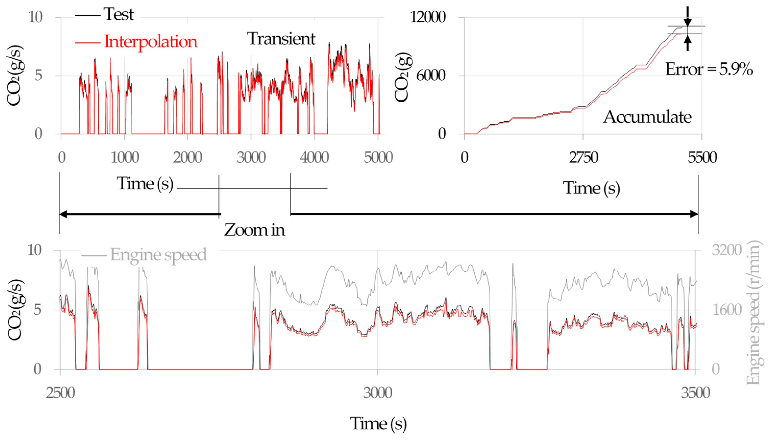
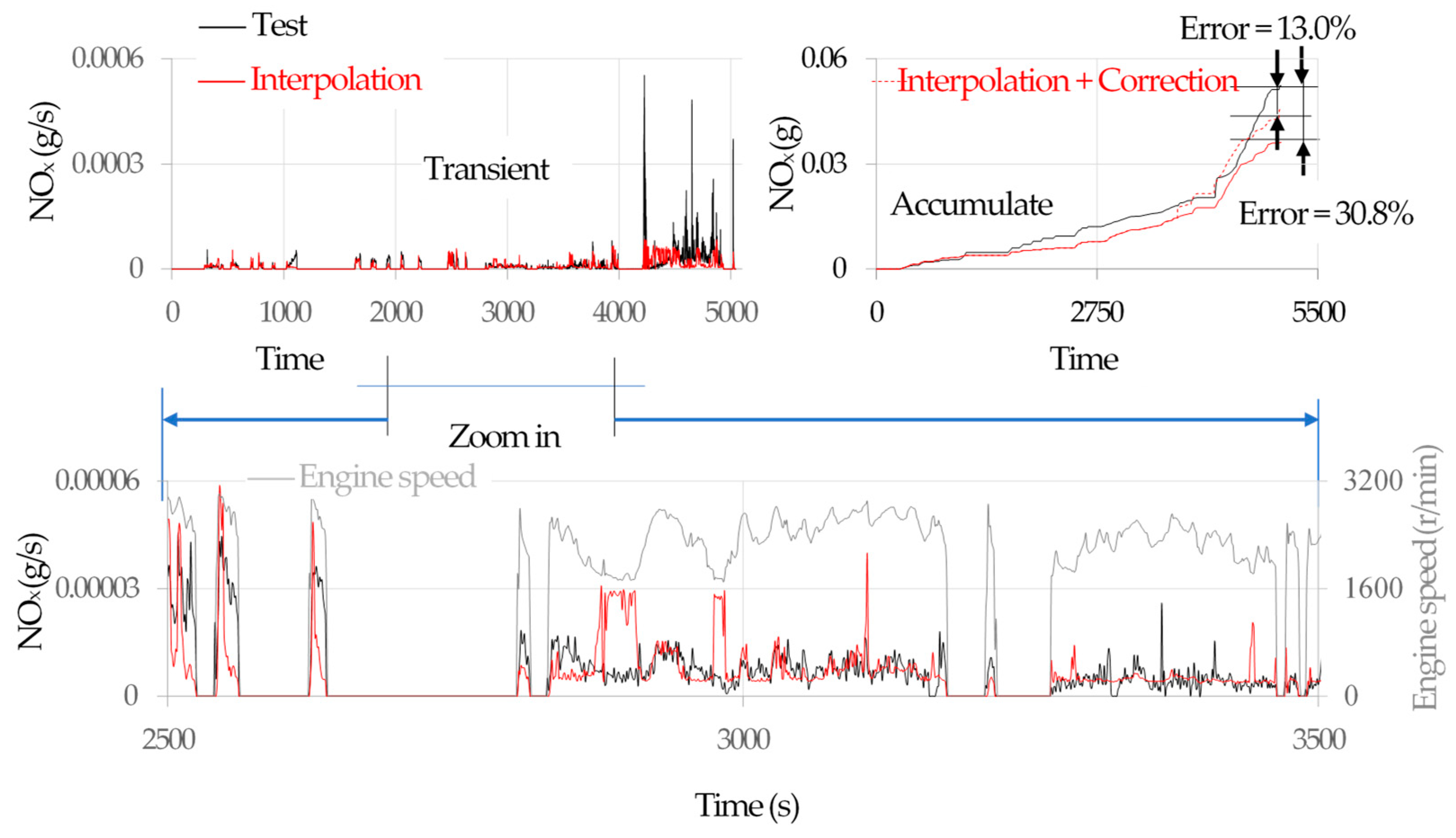
2.2. Real Driving Emission Modeling

The real driving CO₂, CO, NO_x, and PN emissions of the test vehicle in RDE Test A and their accumulation over the total trip are given in Figure 3, Figure 4, Figure 5 and Figure 6, respectively. In these figures, frequent changes in engine operating conditions and many start–stop events can be observed. However, CO₂ emissions seem to be less affected by engine operating dynamics. Using the engine speed and torque recorded in the real driving emission test as input, the steady-state CO₂ emissions can be interpolated in the steady-state CO₂ emission data map from the engine bench tests. Comparing the real driving CO₂ emissions and the interpolated steady-state CO₂ emissions under the same engine speed and torque conditions, it can be found that the difference between the two is not significant. The error of the interpolated total trip cumulative CO₂ emissions relative to the measured data is only 5.9%. In the enlarged view of Figure 3, the engine start–stop events can be recognized by the transient changes in engine speed, but no transient jump-up in CO₂ emissions corresponds to engine start-up; the interpolated CO₂ emissions are still close to the measured CO₂ emissions at the moment when the engine starts up. Thus, the error due to using the interpolated steady-state CO₂ emissions to predict the real driving CO₂ emissions of this EREV should not be too large. In addition, the carbon in the fuel is mainly discharged as CO₂ emissions after in-cylinder chemical reactions (other carbon-containing pollutants in the exhaust are emitted in orders of magnitude lower than CO₂ emissions). Thus, fuel consumption is linearly correlated with CO₂ emissions. This study also uses the interpolated fuel consumption from the engine bench steady-state performance data to predict the real driving fuel consumption.

However, the engine start–stop events significantly affect real driving CO, NO_x, and PN emissions. As shown in Figure 4, some non-continuous singular data points can be observed in the real driving CO emission data, and these singularities are indicative of a tens of times surge in transient CO emissions. In the enlarged view of Figure 4, the moments of these abnormally high CO emission peaks correspond to the engine start-up moments, so the engine start–stop events should cause these abnormally high CO emissions. Since the steady-state engine performance test under laboratory conditions cannot reflect the transient emission characteristics under engine start–stop conditions, a considerable difference exists between the interpolated steady-state CO emissions and the CO emissions caused by the engine start–stop events. In Figure 4, the relative error between the total trip cumulative CO emissions obtained by interpolating the engine steady-state performance data tables and those obtained by cumulating the transient CO emissions in the real driving emission test reaches 29.7%. As for PN emissions, the impact of the engine start–stop events is much more sensitive. In Figure 5, the abnormal transient PN emissions due to the engine start–stop events increase hundreds of times. The total trip cumulative PN emissions obtained by interpolating the engine steady-state performance data tables are less than 10% of those measured in the real driving emissions test, with a relative error of 91.8%. Comparatively, NO_x emissions are less affected by the engine start–stop events. In Figure 6, the abnormal increment of NO_x emissions due to engine start-up is seldom observed in the urban and rural trips, but is only more demonstrated in the motorway trips. The relative error between the interpolated total trip cumulative NO_x emissions and those measured in the real driving emission test is 30.6%. As can be seen, the transient pollutant emissions caused by engine start–stop account for a considerable share of the total pollutant emissions during the actual use of EREVs. Therefore, the severe pollutant emissions from engine start–stops in EREVs should not be ignored.

Because engine speed is decoupled from vehicle speed during EREV driving, the engine operating conditions do not vary much under non-start–stop conditions. In this case, engine operating dynamics have little effect on real driving emissions. Thus, the transient operation of the engine in non-start–stop conditions can be approximated as steady-state operation, and the real driving pollutant emissions under non-start–stop conditions can be calculated by interpolating in the engine steady-state performance data table. Meanwhile, the emission increment of the engine start–stop events is statistically inferred from the emission data samples of the engine start–stop events in the two real driving emission tests. However, the start-up emissions in the two real driving emission tests exhibit strong randomness, and the correlation between the engine start-up emissions and the start–stop event characteristics (e.g., speed, torque, and power during start–stop) is not well defined. In this regard, the statistical mean of the abnormal pollutant emissions associated with the engine start–stop events is considered approximatively as the incremental emissions resulting from a single engine start–stop event. In the real driving emission calculation for the EREV, one start-up emission increment is added when an engine start–stop event is recognized. In contrast, the real driving emissions at the no-start–stop operating points are calculated by interpolating in the engine steady-state performance data tables. Therefore, a new real driving emission modeling method, the interpolated-startup-corrected method, is proposed. It should be noted that since the abnormal NO_x emissions due to the engine start–stop events are mainly manifested in the motorway trip, the above interpolated-startup-corrected NO_x emission models do not work for engine start-up emissions in rural and motorway driving conditions. As shown in Figure 4, Figure 5 and Figure 6, the relative errors between the total trip real driving CO, PN, and NO_x emissions obtained by the interpolated-startup-corrected models and those obtained by the integration of the instantaneous emissions in the real driving emission test are 2.2%, 1.8%, and 13.1%, respectively.

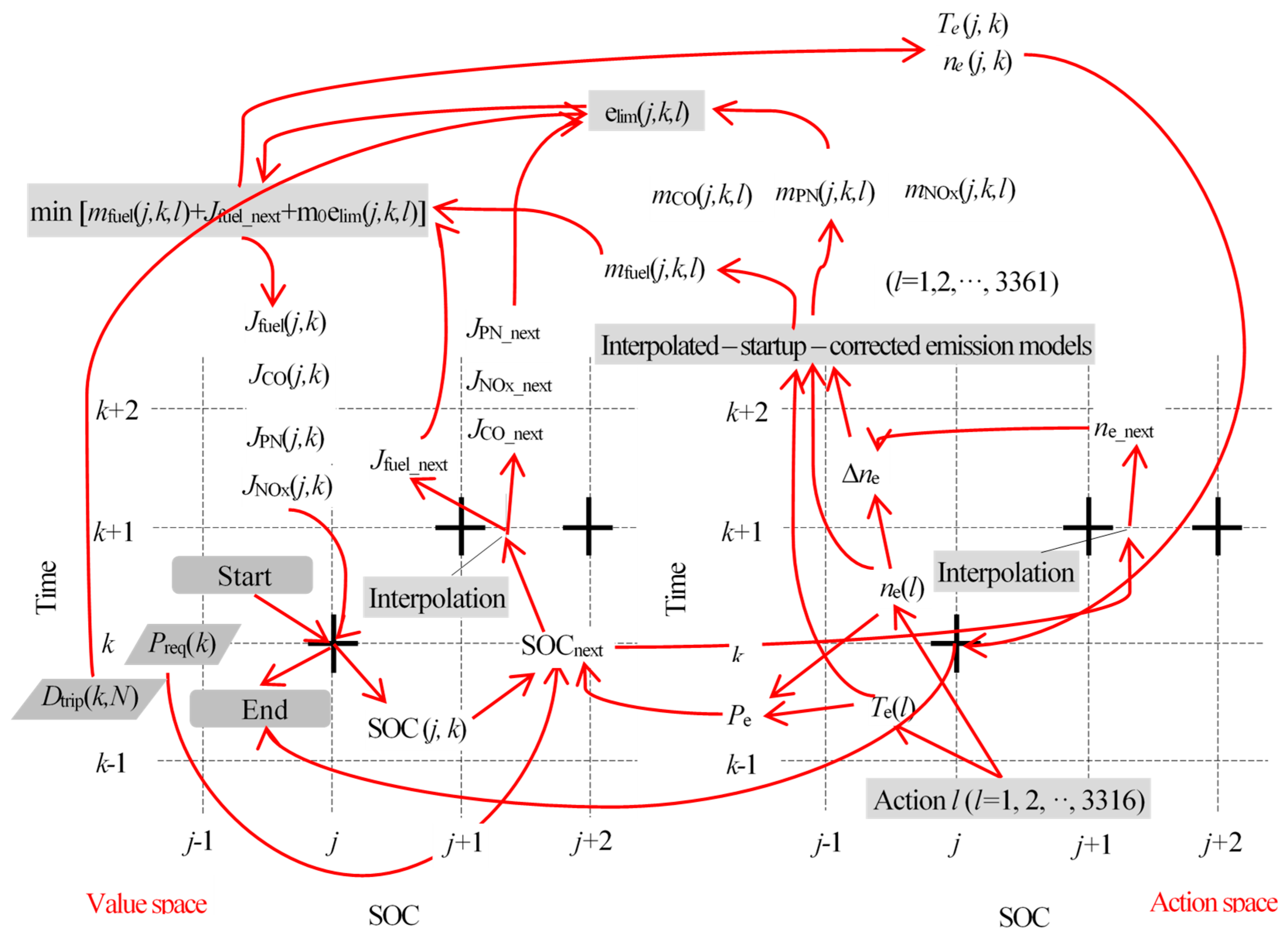
2.3. DP Algorithm with Emission Constraints

The EREV driving history of RDE Test B is considered a time control domain discretized into 5598 grid nodes at a time step of 1 s. Meanwhile, the SOC of the battery is used as a variable to describe the energy system state of the EREV; SOC takes the value range from 0.2 to 0.8, and 6000 grid nodes are divided in the state control domain at the discrete step of 0.0001. In addition, the engine feasible operating domain is also considered an action control domain, where the engine speed range is from 1000 to 4200 r/min and the engine torque range at each speed state is from zero to the maximum value under the wide-open-throttle operating condition. The action control domain is divided into 61 × 51 (speed × torque) grid points with an additional engine shutdown point, so a total of 3316 action discrete points are generated, and each action discrete point corresponds to two engine operating parameters, namely, engine speed (n_e), and torque (T_e), respectively. The optimization of the energy management strategies is the selection of the best engine operating point from the 3316 action discrete points and the corresponding battery SOC in state space so that the value loss function in the control time domain is minimized as the vehicle state is updated from the moment kth to (k + 1)_th:

$$J=\min {\displaystyle {\sum }_{k=1}^{N}L\left(k\right)}$$

(1)

where J is the value loss function in the time control domain, and L(k) is the value loss function at the kth time step, which is determined by SOC, n_e, and T_e at that time step. In the case where the state of charge at the start and end points of the control time domain is determined (i.e., the consumption of externally charged electrical energy remains constant), the fuel consumption can be taken as a value loss, and Equation (1) is transformed into

$$J_{\mathrm{fuel}}=\min {\displaystyle {\sum }_{k=1}^N{m}_{\mathrm{fuel}}\left(k\right)}$$

(2)

where J_fuel is the value loss function scaled by fuel consumption; m_fuel(k) is the fuel consumption at the kth moment, which is determined by n_e and T_e associated with SOC at this time step. When the hazards of pollutant emissions are taken into account, the superior choice of state and action variables is constrained by the emission limits:

$${\displaystyle {\sum }_{k=1}^N{m}_{\mathrm{CO}}\left(k\right)}\le e_{\mathrm{CO}}{D}_{\mathrm{trip}}$$

(3)

$${\displaystyle {\sum }_{k=1}^N{m}_{\mathrm{NOx}}\left(k\right)}\le e_{\mathrm{NOx}}{D}_{\mathrm{trip}}$$

(4)

$${\displaystyle {\sum }_{k=1}^N{m}_{\mathrm{PN}}\left(k\right)}\le e_{\mathrm{PN}}{D}_{\mathrm{trip}}$$

(5)

where m_CO(k), m_NOx(k), and m_PN(k) are the CO, NO_x, and PN emissions at the kth moment, respectively; e_CO, e_NOx, and e_PN are the CO, NO_x, and PN specified-distance emission limits, respectively; and D_trip is the distance traveled by the EREV. Here, m_CO(k), m_NOx(k), and m_PN(k) are also determined by n_e and T_e, which are associated with SOC at the kth time step.

The penalty function method is used to transform the optimization problem of Equations (2)–(5) into another optimization problem without constraints:

$$J_{\mathrm{fuel}}=\min \left[{\displaystyle {\sum }_{k=1}^N{m}_{\mathrm{fuel}}\left(k\right)}+m_{\mathrm{o}}{e}_{\lim }\right]$$

(6)

where m₀ is a sufficiently large positive number with the same dimension as the fuel consumption to act as a penalty; e_lim is the relative difference between the trip emissions and the emission constraint limit, characterizing the positive relative spatial distance beyond the feasible domain constrained by the pollutant emission limits:

$$e_{\lim }={\left[{\left(e_{\lim \mathrm{CO}}\right)}^2+{\left(e_{\lim \mathrm{PN}}\right)}^2+{\left(e_{\lim \mathrm{NOx}}\right)}^2\right]}^{{\displaystyle \frac{1}{2}}}$$

(7)

where e_limCO, e_limPN, and e_limNOx are the projections of e_lim on the CO, PN, and NO_x emission components, respectively, which are defined as

$$e_{\lim \mathrm{CO}}=\left\{\begin{array}{c}{\displaystyle \frac{{\displaystyle {\sum }_{k=1}^N{m}_{\mathrm{CO}}\left(k\right)-e_{\mathrm{CO}}{D}_{\mathrm{trip}}}}{e_{\mathrm{CO}}{D}_{\mathrm{trip}}}}\begin{array}{cc}& if{\displaystyle {\sum }_{k=1}^N{m}_{\mathrm{CO}}\left(k\right)>e_{\mathrm{CO}}{D}_{\mathrm{trip}}}\end{array}\\ 0\begin{array}{cc}& if{\displaystyle {\sum }_{k=1}^N{m}_{\mathrm{CO}}\left(k\right)\le e_{\mathrm{CO}}{D}_{\mathrm{trip}}}\end{array}\end{array}\right.$$

(8)

$$e_{\lim \mathrm{PN}}=\left\{\begin{array}{c}{\displaystyle \frac{{\displaystyle {\sum }_{k=1}^N{m}_{\mathrm{PN}}\left(k\right)-e_{\mathrm{PN}}{D}_{\mathrm{trip}}}}{e_{\mathrm{PN}}{D}_{\mathrm{trip}}}}\begin{array}{cc}& if{\displaystyle {\sum }_{k=1}^N{m}_{\mathrm{PN}}\left(k\right)>e_{\mathrm{PN}}{D}_{\mathrm{trip}}}\end{array}\\ 0\begin{array}{cc}& if{\displaystyle {\sum }_{k=1}^N{m}_{\mathrm{PN}}\left(k\right)\le e_{\mathrm{PN}}{D}_{\mathrm{trip}}}\end{array}\end{array}\right.$$

(9)

$$e_{\lim \mathrm{NOx}}=\left\{\begin{array}{c}{\displaystyle \frac{{\displaystyle {\sum }_{k=1}^N{m}_{\mathrm{NOx}}\left(k\right)-e_{\mathrm{NOx}}{D}_{\mathrm{trip}}}}{e_{\mathrm{NOx}}{D}_{\mathrm{trip}}}}\begin{array}{cc}& if{\displaystyle {\sum }_{k=1}^N{m}_{\mathrm{NOx}}\left(k\right)>e_{\mathrm{NOx}}{D}_{\mathrm{trip}}}\end{array}\\ 0\begin{array}{cc}& if{\displaystyle {\sum }_{k=1}^N{m}_{\mathrm{NOx}}\left(k\right)\le e_{\mathrm{NOx}}{D}_{\mathrm{trip}}}\end{array}\end{array}\right.$$

(10)

Equations (6)–(10) embed the original pollutant emission constraints into the objective function and establish a feasible domain enclosure for pollutant emissions using the penalty function method. The penalty function term is zero when the optimization process is far from the emission constraint boundary; otherwise, the penalty function term is significant. In Equation (6), a value of m₀ that is too small will not act as a penalty, while a value of m₀ that is too large may affect the correct selection of state and action variables that minimize fuel consumption. Therefore, in the solution of the above optimization problem, a smaller m0 can be taken for trial calculation; when the result does not satisfy the constraint conditions of the optimization problem, m₀ is enlarged until the result satisfies the constraint conditions of the optimization problem.

Bellman’s optimality principle indicates that for the optimal strategy of a multi-stage decision problem, by treating any stage and state as the initial stage and the initial state, the remaining strategy from this stage onwards must also be optimal [45]. Accordingly, the DP inverse solution algorithm is as follows: At the Nth time step (N = 5598) in the time control domain, the value function is taken to have an initial value of zero; then, the value loss functions on all SOC grid points are solved inversely from the (N − 1)_th moment to the 1st moment. For the jth SOC grid points in the kth time step, the fuel consumption value loss function is

$$J_{\mathrm{fuel}}\left(j,k\right)=\min \left[m_{fuel}\left(j,k,l\right)+J_{fuel\_next}+m_0{e}_{\lim }\left(j,k,l\right)\right]\begin{array}{cc}& l=1,2,\cdots ,3316\end{array}$$

(11)

where J_fuel(j,k) is the fuel consumption value function at the j-k grid point (the jth SOC grid point of the kth time step), which is the minimum cumulative fuel consumption with j as the initial SOC state in the k to N time control stage; m_fuel(j,k,l) is the fuel consumption at the j-k grid point due to the lth action; J_{fuel_next} is the corresponding fuel consumption value loss function at the (k + 1)_th time step due to the lth action; m₀e_lim(j,k,l) is the penalty function term for limiting pollutant emissions at the j-k grid point. Therein, J_{fuel_next} is calculated by interpolating the fuel consumption value loss functions recorded at the state-time grid points in the (k + 1)_th time step, which needs the battery charge state in the (k + 1)_th time step due to the lth action. This battery charge state is derived from the state transfer equation:

$$SO{C}_{next}=SOC\left(j,k\right)-{\displaystyle \frac{U_{\mathrm{OC}}-{\left(U_{\mathrm{OC}}^2-4R_{\mathrm{int}}{P}_{\mathrm{bat}}\right)}^{\frac{1}{2}}}{2R_{\mathrm{int}}{Q}_{\max }}}$$

(12)

where SOC(j,k) is the battery charge state at the j-k grid point; SOC_next is the battery charge state at the (k + 1)_th moment due to the lth action; U_oc is the open-circuit voltage of the battery, and R_int is the internal resistance of the battery (the relationship between U_oc, R_int, and SOC is obtained from the battery characteristic curves); Q_max is the maximum capacity of the battery; and P_bat is the output or input power of the battery. Since the engine in the EREV can supply electricity directly to the drive motor without going through the battery, the following energy balance relationship is available:

$$P_{\mathrm{bat}}={\displaystyle \frac{P_{\mathrm{dem}}}{{\eta }_{\mathrm{m}}}}-{\eta }_{\mathrm{g}}{P}_{\mathrm{e}}$$

(13)

where P_e is the engine output power, which can be derived from n_e and T_e at the action discrete point; η_g is the generator efficiency taken from the generator efficiency characteristic diagrams; P_dem is the demand power, which is calculated from the real-time motor output speed and torque recorded during RDE Test B; and η_m is the motor efficiency taken from the motor efficiency characteristic diagrams. After obtaining SOC_next, J_{fuel_next} can be calculated by interpolating the fuel consumption value loss function stored at the two grid points neighboring SOC_next on the k + 1 time step. Additionally, in the case that SOC_next calculated by the state transfer equation is outside the SOC range of 0.2–0.8, the action discrete point should be excluded from the action optimization process.

Equation (11) also includes the penalty function term of m₀e_lim(j,k,l), So the pollutant emissions generated by all the actions at the j-k grid point need to be calculated. For the lth action at the j-k grid point, the resulting pollutant emissions can be calculated using the interpolated-startup-corrected emission model. Suppose that the lth action is judged to result in an engine start–stop event. In that case, the interpolated-startup-corrected emission model will additionally include the startup emissions in the resulting pollutant emissions of this action. The engine start–stop event is judged based on the change rate of the engine speed:

$$\mathrm{\Delta }{n}_{\mathrm{e}}>1000\mathrm{r}/\mathrm{m}\mathrm{i}\mathrm{n}$$

(14)

where ∆n_e is the change rate of the engine speed. ∆n_e is the opposite of the difference between the engine speed corresponding to the lth action at the j-k grid point and the engine speed corresponding to the SOC_next state in the (k + 1)_th time step, and the latter can be obtained by interpolating the action information stored in the (k + 1)_th time step.

At the j-k grid point, the pollutant emission value loss functions associated with the lth action are denoted as

$$J_{\mathrm{CO}}\left(j,k\right)=\left[m_{\mathrm{CO}}\left(j,k,l\right)+J_{\mathrm{CO}\text{\_}\mathrm{next}}\right]$$

(15)

$$J_{\mathrm{PN}}\left(j,k\right)=\left[m_{\mathrm{PN}}\left(j,k,l\right)+J_{\mathrm{PN}\text{\_}\mathrm{next}}\right]$$

(16)

$$J_{\mathrm{NOx}}\left(j,k\right)=\left[m_{\mathrm{NOx}}\left(j,k,l\right)+J_{\mathrm{NOx}\text{\_}\mathrm{next}}\right]$$

(17)

where J_CO(j, k), J_PN(j, k), and J_NOx(j, k) are the value loss functions for CO, PN, and NO_x emissions at the j-k grid point, respectively. In essence, J_CO(j, k), J_PN(j, k), and J_NOx(j, k) are the cumulative pollutant emissions when the minimum cumulative fuel consumption in the k to N time control stage is achieved, with j as the initial SOC state. In these equations, m_CO(j,k,l), m_PN(j,k,l), and m_NOx(j,k,l) are CO, PN, and NO_x emissions due to the lth action at the j-k grid point, calculated by the interpolated-startup-corrected emission model; J_{CO_next}, J_{PN_next}, and J_{NOx_next} are the CO, PN, and NO_x emission value loss functions under the SOC_next state in the (k + 1)_th time step, obtained by interpolating the emission value loss functions at the two grid points neighboring SOC_next in the (k + 1)_th time step. For the lth action at the j-k grid point, the positive relative spatial distance between the cumulative pollutant emissions in the k to N time control stage and the pollutant emission limits are

$$e_{\lim }\left(j,k,l\right)={\left\{{\left[e_{\lim \mathrm{CO}}\left(j,k,l\right)\right]}^2+{\left[e_{\mathrm{limPN}}\left(j,k,l\right)\right]}^2+{\left[e_{\lim \mathrm{NOx}}\left(j,k,l\right)\right]}^2\right\}}^{{\displaystyle \frac{1}{2}}}$$

(18)

where e_lim(j,k,l) is the positive relative spatial distance for the lth action at the j-k grid point; e_limCO(j,k,l), e_limPN(j,k,l), and e_limNOx(j,k,l) are the components of e_lim(j,k,l) on the CO, PN, and NO_x emission components, respectively, which are

$$e_{\lim \mathrm{CO}}\left(j,k,l\right)=\left\{\begin{array}{c}{\displaystyle \frac{J_{\mathrm{CO}}\left(j,k\right)-{\mu }_{\mathrm{CO}}{e}_{\mathrm{CO}}{D}_{\mathrm{trip}}\left(k,N\right)}{{\mu }_{\mathrm{CO}}{e}_{\mathrm{CO}}{D}_{\mathrm{trip}}\left(k,N\right)}}\begin{array}{cc}& if\begin{array}{cc}& J_{\mathrm{CO}}\left(j,k\right)>{\mu }_{\mathrm{CO}}{e}_{\mathrm{CO}}{D}_{\mathrm{trip}}\left(k,N\right)\end{array}\end{array}\\ 0\begin{array}{cc}& if\begin{array}{cc}& J_{\mathrm{CO}}\left(j,k\right)\le {\mu }_{\mathrm{CO}}{e}_{\mathrm{CO}}{D}_{\mathrm{trip}}\left(k,N\right)\end{array}\end{array}\end{array}\right.$$

(19)

$$e_{\lim \mathrm{PN}}\left(j,k,l\right)=\left\{\begin{array}{c}{\displaystyle \frac{J_{\mathrm{PN}}\left(j,k\right)-{\mu }_{\mathrm{PN}}{e}_{\mathrm{PN}}{D}_{\mathrm{trip}}\left(k,N\right)}{{\mu }_{\mathrm{PN}}{e}_{\mathrm{PN}}{D}_{\mathrm{trip}}\left(k,N\right)}}\begin{array}{cc}& if\begin{array}{cc}& J_{\mathrm{PN}}\left(j,k\right)>{\mu }_{\mathrm{PN}}{e}_{\mathrm{PN}}{D}_{\mathrm{trip}}\left(k,N\right)\end{array}\end{array}\\ 0\begin{array}{cc}& if\begin{array}{cc}& J_{\mathrm{PN}}\left(j,k\right)\le {\mu }_{\mathrm{PN}}{e}_{\mathrm{PN}}{D}_{\mathrm{trip}}\left(k,N\right)\end{array}\end{array}\end{array}\right.$$

(20)

$$e_{\lim \mathrm{NOx}}\left(j,k,l\right)=\left\{\begin{array}{c}{\displaystyle \frac{J_{\mathrm{NOx}}\left(j,k\right)-{\mu }_{\mathrm{NOx}}{e}_{\mathrm{NOx}}{D}_{\mathrm{trip}}\left(k,N\right)}{{\mu }_{\mathrm{NOx}}{e}_{\mathrm{NOx}}{D}_{\mathrm{trip}}\left(k,N\right)}}\begin{array}{cc}& if\begin{array}{cc}& J_{\mathrm{NOx}}\left(j,k\right)>{\mu }_{\mathrm{NOx}}{e}_{\mathrm{NOx}}{D}_{\mathrm{trip}}\left(k,N\right)\end{array}\end{array}\\ 0\begin{array}{cc}& if\begin{array}{cc}& J_{\mathrm{NOx}}\left(j,k\right)\le {\mu }_{\mathrm{NOx}}{e}_{\mathrm{NOx}}{D}_{\mathrm{trip}}\left(k,N\right)\end{array}\end{array}\end{array}\right.$$

(21)

where D_trip(k, N) is the distance traveled by the vehicle in the k to N period; μ_CO, μ_PN, and μ_NOx are the relaxation factors for the pollutant emission limits at the intermediate time steps, which are co-adjusted with m_o to make the emission limits for the different pollutant emission factors satisfied in the total trip.

Up to this point, m_fuel(j,k,l), J_{fuel_next}, and e_lim(_j,k,l) in Equation (11) are calculated. Thus, at the j-k grid point, an action can be selected from the 3316 action discrete points to allow Equation (11) to hold. After completing the selection of the optimal action at the j-k grid points, J_fuel(j, k), J_CO(j, k), J_PN(j, k), and J_NOx(j, k), as well as n_e and T_e corresponding to the optimization-seeking action, are stored at the j-k grid point. Figure 7 shows the data flow of the action optimization-seeking at the j-k grid point. Subsequently, the action optimization at the next SOC grid point in the same time step continues until the optimization search process at all SOC grid points is completed. After that, the optimization process in the kth time step is repeated in the (k − 1)_th time step, thus completing the action selection at all the SOC grid points in the whole time control domain and ending the DP inverse solution.

Next, in the DP forward solver solution, based on the initial battery SOC at the 1st time step, which is given as the initial condition of the problem, n_e and T_e at this moment are obtained by interpolating the action information stored on the state-time grid points to calculate the engine fuel consumption and output power. Then, SOC at the 2nd time step is obtained by the state transfer equation (Equation (12)), and the action variables at the 2nd time step are solved by interpolating the stored information at the state-time grid points, the change rate of the engine speed is calculated, and the interpolated-startup-corrected emission models obtain the CO, PN, and NO_x emissions. The above process continues in a loop until the computation of states and actions on all time steps in the control time domain is completed in the time-forward direction. In this process, the EREV energy management strategies constrained by real driving emissions and aimed at minimizing fuel consumption in the control time domain are investigated.

3. Results and Discussions

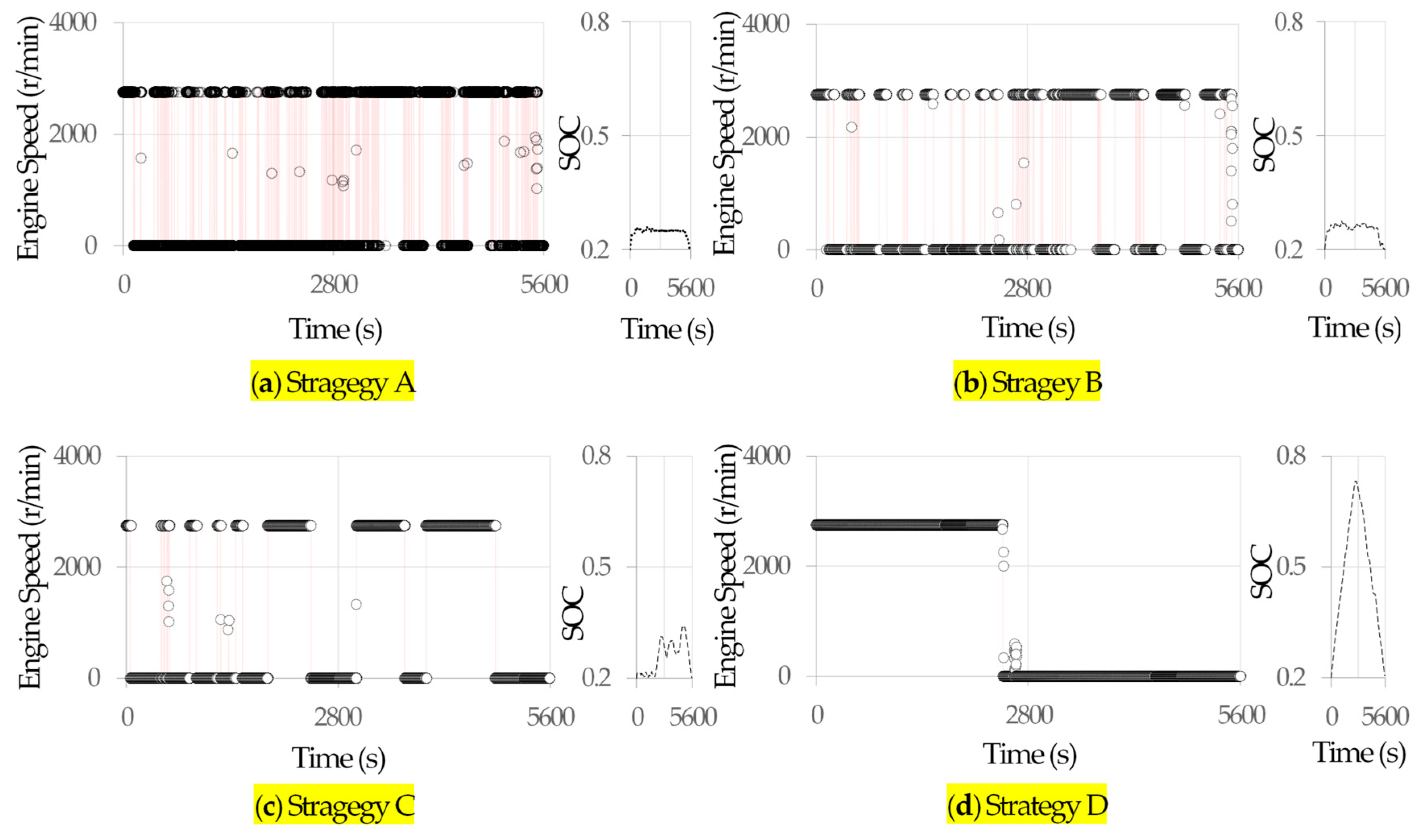
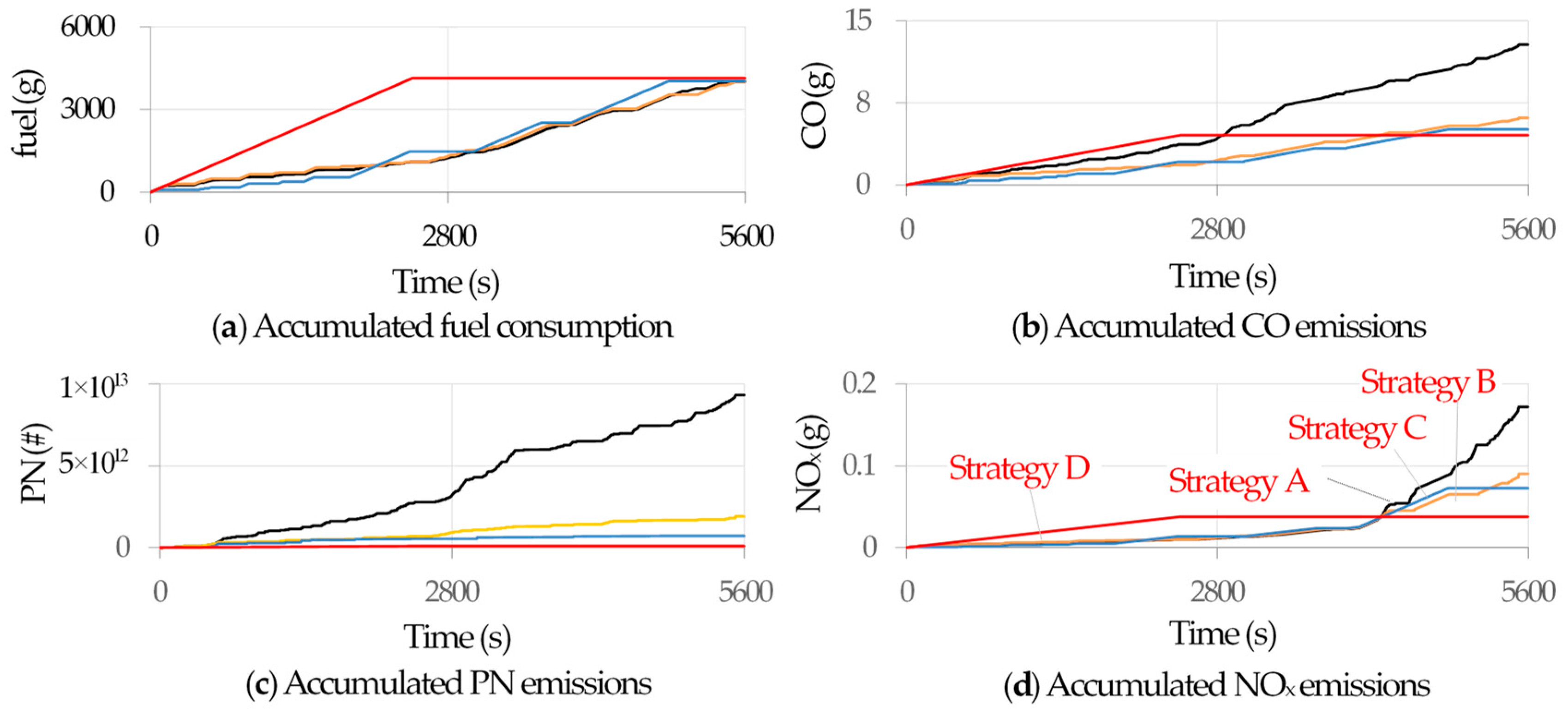
3.1. Start–Stop Reduction Strategies

Figure 8 shows the numerical solutions given by the DP algorithm to tighten the pollutant emission limits step by step. The SOC is 0.2 at the test trip’s start. The emission limits are initially 0.5 g/km for CO, 6 × 10¹¹#/km for PN, and 0.035 g/km for NO_x. Due to the more extensive initial setup, these emission limits do not constrain the optimization strategy that targets fuel consumption. In this strategy (Strategy A), the engine runs at the lowest fuel consumption rate condition (2750 r/min × 99.72 N·m) or stops. As shown by the engine speed curve in Figure 8a, the engine essentially operates only at two-speed condition points, 0 and 2750 r/min. Moreover, the engine output power should be as close as possible to the driving demand power to reduce the charging and discharging of the battery and avoid the losses of energy conversion between electrical energy and chemical energy. To do this power following, the engine frequently switches between these two operating conditions. Since the change in SOC indicates the difference between the engine output power and the driving demand power, the SOC varies only in a tiny range close to 0.2, as noted in the SOC curve in Figure 8a. In addition, a few singular operating points occur during the engine start–stop transients, which are neither at the lowest fuel consumption rate nor in the engine shutdown condition. However, these singular operating points are only about 3 in a thousand and decrease with the reduction of start–stop events or finer SOC grids. Accordingly, these singular operating points are due to interpolation errors in the DP algorithm.

As the pollutant emission limits become stricter, Strategy B, Strategy C, and Strategy D, given by the DP algorithm with emission constraints, are still to maintain the operating points at the lowest fuel consumption rate condition and the engine stop condition. However, the engine start–stop events are reduced, and the SOC variations are increased, as shown in Figure 8b–d. When pollutant emissions are further restricted, start–stop events are no longer observed. In Figure 8d, Strategy D is a no-start–stop strategy given by the DP solution. Strategy D allows the engine to run at the lowest fuel consumption rate and charge the battery in the initial part of the trip (within the 0 to 2467 s period). Then, the engine is shut down, and purely electrical driving is used during the trip’s latter part (within the 2468 to 5579 s time period). The SOC curves in Figure 8d also reflect the charging and discharging characteristics of the no-start–stop strategy. At the end of the first half of the trip, SOC reaches a peak value close to 0.8. Therefore, applying a non-start–stop strategy may be compromised in the case of small battery capacities. Overall, since fuel consumption is not sensitive to engine start–stop events, the cumulative fuel consumption of the no-start–stop strategy in Figure 8d does not differ much from that in Figure 8a–c, except for a small amount of energy loss due to the increased battery charging and discharging, as shown in Figure 9a. However, pollutant emissions are significantly affected by engine start–stop events. Compared to Strategy A, which is without the emission constraints, the CO and NO_x emissions under the no-start–stop strategy are only about 30% of the former; the PN emissions are even orders of magnitude lower, as shown in Figure 9b–d. Therefore, the start–stop reduction strategies given by the DP algorithm can significantly reduce real driving emissions while maintaining the fuel economy advantage.

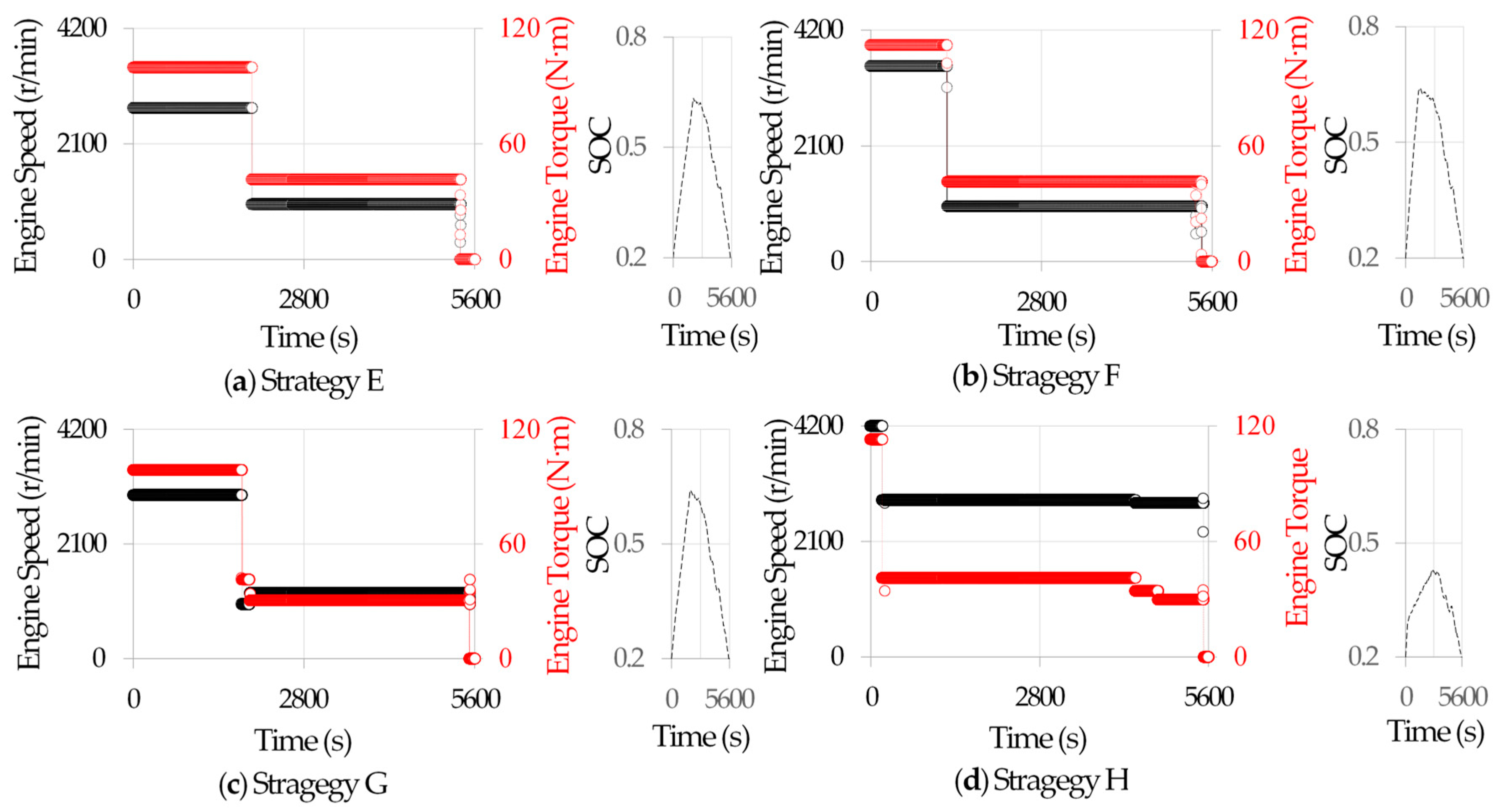
3.2. Condition Migration Strategies

Since the engine’s operating state is decoupled from the vehicle’s driving state under real driving conditions, the engine can operate under lower pollutant emission rate conditions to reduce pollutant emissions. As the emission limits progressively tighten, some engine operating points can migrate from the lowest fuel consumption to the lower pollutant emission rate conditions. As can be seen, these engine condition migrations tighten emission limits at the expense of fuel economy; also, the operating conditions for the lower emission rates of different pollutants do not overlap. These two factors make the engine condition migration more challenging to decide. To this end, the DP algorithm provides condition migration strategies that provide solutions to achieve a reasonable compromise between fuel consumption reduction and pollutant emission reduction.

Figure 10 shows the DP solution for the stricter CO and NO_x emission limits by engine condition migration. Given that the PN emissions have already achieved orders of magnitude lower reductions through the start–stop reduction strategy, the PN emissions are not discussed as being more restricted in the condition migration strategies. In Figure 10a, Strategy E given by the DP algorithm migrates the operating points located within the 1949 to 5366 s time period from the lowest fuel consumption rate condition and the engine stop condition to the lowest CO emission rate condition (1000 r/min × 41.46 N·m), so that the CO emissions less than those obtained by the non-start–stop strategy are obtained. To continue to tighten the CO emissions while liberalizing PN and NO_x emissions, the DP algorithm gives Strategy F, which migrates more operating points located within the 1251 to 5431 s time period from the lowest fuel consumption rate condition to the lowest CO emission rate condition. Due to the low output power at the lowest CO emission rate condition, the operating points located within the 0 to 1251 s time period deviate from the lowest fuel consumption rate condition and relocate at the higher engine speed and torque condition (3550 r/min × 121.22 N·m) to compensate for the reduction of engine output power, as shown in Figure 10b. With this strategy, the total trip CO emissions are slightly reduced, but PN emissions, NO_x emissions, and fuel consumption increase significantly, as shown in Figure 11.

Figure 10c shows Strategy G given by the DP algorithm to further limit NOx emissions. Under this strategy, the operating points located within the 1787 to 5517 s time period are migrated from the lowest CO emission rate condition to the higher speed and lower torque condition (1200 r/min × 30.38 N·m); also, the operating points located within the 0 to 1786 s time period are migrated from the lowest fuel consumption rate condition to the higher speed and lower torque condition (3000 r/min × 98.83 N·m). Generally, higher engine speeds contribute to higher power output, while lower engine loads favor lower NO_x emissions. Compared to the case in Figure 10a, the total trip NO_x emissions and PN emissions under this strategy show a significant reduction, with little change in CO emissions and a slight increase in fuel consumption, as seen in Figure 11. In addition, Figure 10d shows Strategy H for further limiting NO_x emissions while liberalizing CO and PN emissions. In the strategy, the engine almost operates in the region around the condition with the higher speed and lower torque (2850 r/min × 41.14 N·m). The operating duration of the high speed and high torque conditions (4200 r/min × 113.02 N·m) is significantly shorter, only within the 0 to 189 s time period. These actions contribute to the reduction of NO_x emissions. As shown in Figure 11, the NO_x emissions are reduced considerably as expected; however, the CO emissions, PN emissions, and fuel consumption are significantly increased, and the overall performance is worse than that of Strategy G in Figure 10c. Comparing the no-start–stop strategy in Figure 8d with the condition migration strategy in Figure 10c, the latter has significantly lower trip pollutant emissions than the former but slightly higher fuel consumption, as shown in Figure 9 and Figure 11. It can be seen that the condition migration strategies can reasonably compromise fuel economy and pollutant emissions concerning the preset emission limits, thus possibly limiting pollutant emissions beyond the start–stop reduction strategy.

4. Conclusions

During actual driving, the engine, as a range extender of EREV, frequently switches between efficient operating and shutdown conditions, generating many start–stop events that sharply increase pollutant emissions. Considering the limits on real driving emissions in energy management strategies is crucial. To this end, the interpolated-startup-corrected emission models are proposed, which approximate the real driving emissions under the non-start–stop condition by interpolating the engine steady-state performance maps and statistically infer the abnormal engine start-up emissions based on the recorded emissions in the real driving emission tests. The resulting interpolated-startup-corrected emission models are verified to agree well with the tested real driving emissions.

The optimization problem is constructed with fuel consumption as the objective and real driving emissions as the constraints and is transformed into an unconstrained one by the penalty function method. To solve the optimization problem, the DP algorithm combined with the interpolated-startup corrected emission models is developed by inventing multiple interpolation operations in the value-space and action-space domains. The DP algorithm provides start–stop reduction strategies and condition migration strategies. The start–stop reduction strategies suggest gradually reducing the engine start–stop events as the emission limits are tightened. On this basis, the condition migration strategies indicate how to relocate the engine operating points to compromise the fuel economy and pollutant emission targets. Several DP solutions are interpreted reasonably, confirming the developed DP algorithm’s correctness and effectiveness.

Based on a new approach that has never been attempted before, this study constructs the emission models from real driving emission test data and then integrates the emission models into the DP optimization of EREV energy management strategies while considering the control of pollutant emissions. It is confirmed that the simultaneous optimization of energy consumption and emissions brings significant overall economic and social benefits to EREVs. Although the DP algorithm cannot be directly implemented in real time, it can be used to obtain theoretically optimal control results and as a benchmark for evaluating the control performance resulting from other real-time energy management strategies. The study’s next step will consider combining such real driving emission models that can reflect the dynamic effects of operating conditions with real-time optimization algorithms, such as DRL algorithms, to promote the development of EREV energy management strategies.

References

1. Cherp, A.; Jewell, J. The concept of energy security: Beyond the four As. Energy Policy 2014, 75, 415–421. [Google Scholar] [CrossRef]
2. Lu, Z.N.; Chen, H.Y.; Hao, Y.; Wang, J.Y.; Song, X.J.; Mok, T.M. The dynamic relationship between environmental pollution, economic development and public health: Evidence from China. J. Clean. Prod. 2017, 166, 134–147. [Google Scholar] [CrossRef]
3. Jorgenson, A.K.; Fiske, S.; Hubacek, K.; Li, J.; McGovern, T.; Rick, T.; Schor, J.B.; Solecki, W.; York, R.; Zycherman, A. Social science perspectives on drivers of and responses to global climate change. Wires Clim. Chang. 2019, 10, e554. [Google Scholar] [CrossRef] [PubMed]
4. Zelasky, S.E.; Buonocore, J.J. The social costs of health- and climate-related on-road vehicle emissions in the continental United States from 2008 to 2017. Environ. Res. Lett. 2021, 16, 065009. [Google Scholar] [CrossRef]
5. Andwari, A.M.; Pesiridis, A.; Rajoo, S.; Martinez-Botas, R.; Esfahanian, V. A review of battery electric vehicle technology and readiness levels. Renew. Sustain. Energy Rev. 2017, 78, 414–430. [Google Scholar] [CrossRef]
6. Liu, Z.W.; Hao, H.; Cheng, X.; Zhao, F.Q. Critical issues of energy efficient and new energy vehicles development in China. Energy Policy 2018, 115, 92–97. [Google Scholar] [CrossRef]
7. Ku, A.; Kammen, D.M.; Castellanos, S. A quantitative, equitable framework for urban transportation electrification: Oakland, California as a mobility model of climate justice. Sustain. Cities Soc. 2021, 74, 103179. [Google Scholar] [CrossRef]
8. Puma-Benavides, D.S.; Izquierdo-Reyes, J.; Calderon-Najera, J.D.; Ramirez-Mendoza, R.A. A Systematic Review of Technologies, Control Methods, and Optimization for Extended-Range Electric Vehicles. Appl. Sci. 2021, 11, 7095. [Google Scholar] [CrossRef]
9. Zhao, F.Q.; Liu, X.L.; Hao, H.; Liu, Z.W. A comprehensive study of range-extended electric vehicles from the perspectives of the technology, policy, market, and design concept. Int. J. Vehicle Des. 2023, 92, 190–212. [Google Scholar] [CrossRef]
10. Prasad, S.L.; Gudipalli, A. Range-anxiety reduction strategies for extended-range electric vehicle. Int. Trans. Electr. Energy Syst. 2023, 2023, 7246414. [Google Scholar]
11. Tate, E.D.; Harpster, M.O.; Savagian, P.J. The electrification of the automobile: From conventional hybrid, to plug-in hybrids, to extended-range electric vehicles. SAE Int. J. Passeng. Cars-Electron. Electr. Syst. 2008, 1, 125–135. [Google Scholar] [CrossRef]
12. Pozzato, G.; Formentin, S.; Panzani, G.; Savaresi, S.M. Least costly energy management for extended-range electric vehicles: An economic optimization framework. Eur. J. Control 2020, 56, 218–230. [Google Scholar] [CrossRef]
13. Wu, J.L.; Gao, W.H.; Zhang, Y.Q. A new real-time optimal energy management strategy for range extended electric vehicles considering battery degradation and engine start-up. Adv. Mech. Eng. 2024, 16, 16878132241257327. [Google Scholar] [CrossRef]
14. Hu, D.; Huang, C.; Yin, G.D.; Li, Y.M.; Huang, Y.; Huang, H.L.; Wu, J.D.; Li, W.F.; Xie, H. A transfer-based reinforcement learning collaborative energy management strategy for extended-range electric buses with cabin temperature comfort consideration. Energy 2024, 290, 130097. [Google Scholar] [CrossRef]
15. Xiao, B.; Ruan, J.; Yang, W.; Walker, P.D.; Zhang, N. A review of pivotal energy management strategies for extended range electric vehicles. Renew. Sustain. Energy Rev. 2021, 149, 111194. [Google Scholar] [CrossRef]
16. Turker, E.; Bulut, E.; Kahraman, A.; Cakici, M.; Ozturk, F. Estimation of energy management strategy using neural-network-based surrogate model for range extended vehicle. Appl. Sci. 2023, 12, 12935. [Google Scholar] [CrossRef]
17. Du, J.Y.; Chen, J.F.; Song, Z.Y.; Gao, M.M.; Ouyang, M.G. Design method of a power management strategy for variable battery capacities range-extended electric vehicles to improve energy efficiency and cost-effectiveness. Energy 2017, 121, 32–34. [Google Scholar] [CrossRef]
18. Kalia, A.V.; Fabien, B.C. Comparison of model predictive control and distance constrained-adaptive concurrent dynamic programming algorithms for extended range electric vehicle optimal energy management. J. Dyn. Syst. Meas. Control 2021, 143, 094504. [Google Scholar] [CrossRef]
19. Zhang, Y.; Li, Q.X.; Wen, C.Q.; Liu, M.M.; Yang, X.H.; Xu, H.M.; Li, J. Predictive equivalent consumption minimization strategy based on driving pattern personalized reconstruction. Appl. Energy 2024, 367, 123424. [Google Scholar] [CrossRef]
20. Xi, L.H.; Zhang, X.; Sun, C.Y.; Wang, Z.X.; Hou, X.S.; Zhang, J.B. Intelligent energy management control for extended range electric vehicles based on dynamic programming and neural network. Energies 2017, 10, 1871. [Google Scholar] [CrossRef]
21. Yu, Y.B.; Jiang, J.Y.; Min, H.T.; Zhang, Z.P.; Sun, W.Y.; Cao, Q.M. Integrated energy and thermal management strategy for extended range electric vehicle based on battery temperature and state-of-charge global planning. Energy Convers. Manag. 2023, 288, 117154. [Google Scholar] [CrossRef]
22. Xiao, B.Y.; Yang, W.W.; Wu, J.M.; Walker, P.D.; Zhang, N. Energy management strategy via maximum entropy reinforcement learning for an extended range logistics vehicle. Energy 2022, 253, 124105. [Google Scholar] [CrossRef]
23. Sun, Z.Y.; Guo, R.; Xue, X.; Hong, Z.; Luo, M.H.; Wong, P.K.; Liu, J.J.R.; Wang, X.Z. Application-oriented mode decision for energy management of range-extended electric vehicle based on reinforcement learning. Electr. Power Syst. Res. 2024, 226, 109896. [Google Scholar] [CrossRef]
24. Yao, M.Y.; Zhu, B.; Zhang, N. Adaptive real-time optimal control for energy management strategy of extended range electric vehicle. Energy Convers. Manag. 2021, 234, 113874. [Google Scholar] [CrossRef]
25. Yang, Y.; Zhang, Y.T.; Tian, J.Y.; Li, T. Adaptive real-time optimal energy management strategy for extender range electric vehicle. Energy 2022, 197, 117237. [Google Scholar] [CrossRef]
26. Krawczyk, P.; Kopczynski, A.; Lasocki, J. Modeling and simulation of extended-range electric vehicle with control strategy to assess fuel consumption and CO2 emission for the expected driving range. Energies 2022, 15, 4187. [Google Scholar] [CrossRef]
27. Lin, W.Y.; Zhao, H.; Zhang, B.Z.; Wang, Y.; Xiao, Y.; Xu, K.; Zhao, R. Predictive energy management strategy for range-extended electric vehicles based on ITS information and start-stop optimization with vehicle velocity forecast. Energies 2022, 15, 7774. [Google Scholar] [CrossRef]
28. Wang, Y.X.; Lou, D.M.; Xu, N.; Fang, L.; Tan, P.Q. Energy management and emission control for range extended electric vehicles. Energy 2021, 236, 121370. [Google Scholar] [CrossRef]
29. Liu, H.W.; Lei, Y.L.; Fu, Y.; Li, X.Z. A novel hybrid-point-line energy management strategy based on multi-objective optimization for range-extended electric vehicle. Energy 2022, 247, 123357. [Google Scholar] [CrossRef]
30. Lin, X.Y.; Chen, Z.Y.; Zhang, J.J.; Wu, C.Y. A multi-objective optimization control strategy of a range-extended electric vehicle for the trip range and road gradient adaption. Int. J. Automot. Technol. 2024, 25, 131–145. [Google Scholar] [CrossRef]
31. Chang, C.; Fan, Z.K.; Wang, Z.H.; Liu, H.W. Research on adaptive two-point energy management strategy and optimization for range-extended electric vehicle. IEEE Access 2023, 11, 90201–90213. [Google Scholar] [CrossRef]
32. Tang, X.L.; Chen, J.X.; Liu, T.; Qin, Y.C.; Cao, D.P. Distributed deep reinforcement learning-based energy and emission management strategy for hybrid electric vehicles. IEEE Trans. Veh. Technol. 2021, 70, 9922–9934. [Google Scholar] [CrossRef]
33. Giakoumis, E.G.; Alafouzos, A.I. Study of diesel engine performance and emissions during a transient cycle applying an engine mapping-based methodology. Appl. Energy 2010, 87, 1358–1365. [Google Scholar] [CrossRef]
34. Fu, J.Q.; Deng, B.L.; Liu, X.Q.; Shu, J.; Xu, Y.; Liu, J.P. The experimental study on transient emissions and engine behaviors of a sporting motorcycle under world motorcycle test cycle. Energy 2020, 211, 118670. [Google Scholar] [CrossRef]
35. Gallus, J.; Kirchner, U.; Vogt, R.; Benter, T. Impact of driving style and road grade on gaseous exhaust emissions of passenger vehicles measured by a portable emission measurement system (PEMS). Transp. Res. Part D Transp. Environ. 2017, 52, 215–226. [Google Scholar] [CrossRef]
36. Huang, R.; Ni, J.M.; Zheng, T.; Wang, Q.W.; Shi, X.Y.; Cheng, Z.X. Characterizing and assessing the fuel economy, particle number and gaseous emissions performance of hybrid electric and conventional vehicles under different driving modes. Atmos. Pollut. Res. 2022, 13, 101597. [Google Scholar] [CrossRef]
37. Shahariar, G.M.H.; Bodisco, T.A.; Zare, A.; Sajjad, M.; Jahirul, M.I.; Van, T.C.; Bartlett, H.; Ristovski, Z.; Brown, R.J. Impact of driving style and traffic condition on emissions and fuel consumption during real transient operation. Fuel 2022, 319, 123874. [Google Scholar] [CrossRef]
38. Khan, T.; Frey, H.C. Comparison of real and certification emission rates for light duty gasoline vehicles. Sci. Total Environ. 2018, 622, 790–800. [Google Scholar] [CrossRef] [PubMed]
39. Triantafyllopoulos, G.; Dimaratos, A.; Ntziachristos, L.; Bernard, Y.; Dornoff, J.; Samaras, Z. A study on the CO2 and NOx emissions performance of Euro 6 diesel vehicles under various chassis dynamometer and on-road conditions including latest regulatory provisions. Sci. Total Environ. 2019, 666, 337–346. [Google Scholar] [CrossRef]
40. Jimenez, J.L.; Valido, J.; Molden, N. The drivers behind differences between official and actual vehicle efficiency and CO2 emissions. Transp. Res. Part D Transp. Environ. 2019, 67, 628–641. [Google Scholar] [CrossRef]
41. Du, B.C.; Zhang, L.; Zou, J.; Han, J.L.; Zhang, Y.; Xu, H.L. Investigating the impact of route topography on real driving emission tests based on large data sample at data window level. Sci. Total Environ. 2022, 809, 151133. [Google Scholar] [CrossRef] [PubMed]
42. Barbier, A.; Salavert, J.M.; Palau, C.E.; Guardiola, C. Analysis of the Euro 7 on-board emissions monitoring concept with real-driving data. Transp. Res. Part D Transp. Environ. 2024, 127, 104062. [Google Scholar] [CrossRef]
43. European Commission (EC). Commission Regulation (EU) 2023/443 of 8 February 2023 amending Regulation (EU) 2017/1151 as regards the emission type approval procedures for light passenger and commercial vehicles. Off. J. Eur. Union 2023. Available online: https://eur-lex.europa.eu/eli/reg/2023/443/oj/eng (accessed on 24 December 2024).
44. GB18352.6-2016; Limits and Measurement Methods for Emissions from Light-Duty Vehicles (CHINA VI). China Environmental Science Press: Beijing, China, 2016.
45. Bellman, R.E.; Dreyfus, S.E. Applied Dynamic Programming; Princeton University Press: Princeton, NJ, USA, 1962. [Google Scholar]
Figure 1. Test vehicle and on-board PEMS: 1—Gas analyzer module, 2—Filter unit, 3—Pitot tube flow meter module, 4—Power management module, 5—PN measurement module, 6—System control unit, 7—Gas sampling tube, 8—PN sampling tube, 9—Exhaust temperature sensor, 10—Pitot tube, 11—Tail-pipe attachment.
Applsci 15 00142 g001
Figure 2. Speed and altitude profiles of the two RDE tests.
Applsci 15 00142 g002
Figure 3. Real driving CO2 emissions associated with the engine’s start–stop events.
Applsci 15 00142 g003
Figure 4. Real driving CO emissions associated with the engine’s start–stop events.
Applsci 15 00142 g004
Figure 5. Real-driving PN emissions associated with the engine’s start–stop events.
Applsci 15 00142 g005
Figure 6. Real-driving NOx emissions associated with the engine’s start–stop events.
Applsci 15 00142 g006
Figure 7. Data flow of the action optimization-seeking at the j-k grid point.
Applsci 15 00142 g007
Figure 8. Start-stop reduction strategies to tighten the pollutant emission limits.
Applsci 15 00142 g008
Figure 9. Accumulated real driving emissions of the start–stop reduction strategies.
Applsci 15 00142 g009
Figure 10. Condition migration strategies to tighten the pollutant emission limits.
Applsci 15 00142 g010
Figure 11. Accumulated real driving emissions of the condition migration strategies.
Applsci 15 00142 g011
Disclaimer/Publisher’s Note: The statements, opinions and data contained in all publications are solely those of the individual author(s) and contributor(s) and not of MDPI and/or the editor(s). MDPI and/or the editor(s) disclaim responsibility for any injury to people or property resulting from any ideas, methods, instructions or products referred to in the content.