Imputing Covariance for Meta-Analysis in the Presence of Interaction

Abstract

Detecting interactions is a critical aspect of medical research. When interactions are present, it is essential to calculate confidence intervals for both the main effect and the interaction effect. This requires determining the covariance between the two effects. In a two-stage individual patient data (IPD) meta-analysis, the coefficients, as well as their variances and covariances, can be calculated for each study. These coefficients can then be combined into an overall estimate using either a fixed-effect or random-effects meta-analysis model. The overall variance of the combined coefficient is typically derived using the inverse-variance method. The most commonly used method for calculating the overall covariance between the main effect and the interaction effect in meta-analysis is multivariate meta-analysis. In this paper, we propose an alternative, straightforward, and transparent method for calculating this covariance when interactions are considered in a meta-analysis. To facilitate implementation, we have developed an R package, ‘covmeta’.

1. Introduction

When conducting an individual patient data (IPD) meta-analysis, researchers may need to examine interactions between two predictors [1,2]. In a one-stage meta-analysis [3], all data are combined into a single dataset before analysis, allowing for the calculation of the covariance between predictors. However, this approach may not be feasible in situations where data cannot be consolidated into a single dataset, such as when data-sharing restrictions prevent data transfer. In such cases, a two-stage IPD meta-analysis is necessary [4].

When interactions are present, it is crucial to calculate confidence intervals for both the combined main effect and the interaction effect [5]. Additionally, determining the overall covariance between the two coefficients for combined effects in two-stage IPD meta-analyses is vital.

The most commonly used method for calculating the overall covariance between the main effect and the interaction effect in meta-analysis is multivariate meta-analysis [6,7,8]. In this paper, we propose an alternative, straightforward, and transparent method for calculating this covariance when interactions are considered in a meta-analysis. This method is applicable to both fixed-effect and random-effects meta-analysis models, providing a practical solution for researchers analyzing interactions within a meta-analytic framework.

2. Regression with Interaction

Suppose we aim to conduct a meta-analysis to explore the interaction between falls and age and investigate whether the effect of falls on hip fractures varies across different age levels. (Note: This example is for illustrative purposes only and is not intended to provide any evidence on the topic.) A Poisson regression model can be utilized to examine these effects.

The Poisson model is specified as follows

$$Y_i\sim Poisson\left({\mu }_i\right)$$

(1)

with the following log-linear relationship

$$\begin{array}{cc}\hfill log\left({\mu }_i\right)& ={\widehat{\beta }}_0+{\widehat{\beta }}_1\times fall+{\widehat{\beta }}_2\times (fall\times age)+{\widehat{\beta }}_3\times age\hfill \\ & ={\widehat{\beta }}_0+({\widehat{\beta }}_1+{\widehat{\beta }}_2\times age)\times fall+{\widehat{\beta }}_3\times age\hfill \end{array}$$

The effect of falls can be calculated as

$$\begin{array}{cc}\hfill \beta & =log\left({\mu }_{fall=1}\right)-log\left({\mu }_{fall=0}\right)\hfill \\ & =[{\widehat{\beta }}_0+({\widehat{\beta }}_1+{\widehat{\beta }}_2\times age)\times 1+{\widehat{\beta }}_3\times age]-[{\widehat{\beta }}_0+({\widehat{\beta }}_1+{\widehat{\beta }}_2\times age)\times 0+{\widehat{\beta }}_3\times age]\hfill \\ & =({\widehat{\beta }}_1+{\widehat{\beta }}_2\times age)\hfill \end{array}$$

(2)

If exponentiating $\beta$ yields the rate ratio (RR) for the effect.

The effect of falls depends on $({\widehat{\beta }}_1+{\widehat{\beta }}_2\times age)$, and its $(1-\alpha )100\%$ confidence interval can be calculated as [5]

$$({\widehat{\beta }}_1+{\widehat{\beta }}_2\times age)\pm t_{n-p-1,\alpha /2}\sqrt{var\left({\widehat{\beta }}_1\right)+ag{e}^2\times var\left({\widehat{\beta }}_2\right)+2\times age\times cov({\widehat{\beta }}_1,{\widehat{\beta }}_2)}$$

(3)

In this model, n represents the sample size, p denotes the number of predictors, and for large samples, the t score can be approximated by the z score. The variable ‘age’ serves as an effect modifier.

For a two-stage meta-analysis, the overall effects and variances of ${\widehat{\beta }}_1$ and ${\widehat{\beta }}_2$ can be calculated using the inverse-variance weighted average method [9,10,11,12]. Moreover, when investigating interactions, it is crucial to combine these two regression coefficients to construct confidence intervals for the effect of falls across different age levels.

We present a method for combining coefficients and their covariance in a two-stage meta-analysis when interactions are present.

Suppose we have data from 10 cohort studies. For each cohort, we fit the specified Poisson regression model and obtain the following results.

In

Table 1. Simulated results for 10 cohort studies.

Cohort	${\widehat{\mathit{\beta }}}_{1\mathit{i}}$	${\widehat{\mathit{\beta }}}_{2\mathit{i}}$	var(${\widehat{\mathit{\beta }}}_{1\mathit{i}}$)	var(${\widehat{\mathit{\beta }}}_{2\mathit{i}}$)	cov(${\widehat{\mathit{\beta }}}_{1\mathit{i}},{\widehat{\mathit{\beta }}}_{2\mathit{i}}$)	${\mathit{n}}_{\mathit{i}}$
A	3.0014	−0.0240	2.9419	0.0005	−0.0333	5000
B	1.1488	−0.0677	14.6165	0.0029	−0.2000	30,000
C	1.5819	−0.0936	15.8097	0.0022	−0.1825	10,000
D	2.0349	−0.0139	3.6954	0.0318	−0.3230	3000
E	−4.1219	0.0225	5.2448	0.0009	−0.0629	2000
F	1.2506	−0.0020	11.2628	0.002	−0.144	5000
G	2.3383	−0.0173	5.2458	0.0009	−0.0644	1000
H	−3.1343	0.0483	9.0698	0.0013	−0.103	2000
I	1.3066	−0.0005	13.7763	0.0031	−0.2000	800
J	3.7753	−0.021	15.0422	0.0019	−0.1635	3200

, ${\widehat{\beta }}_{1i}$ represents the coefficient for falls (i.e., the main effect) in the ith cohort, while ${\widehat{\beta }}_{2i}$ corresponds to the interaction effect of fall × age. $\mathrm{var}\left({\widehat{\beta }}_{1i}\right)$ and $\mathrm{var}\left({\widehat{\beta }}_{2i}\right)$ denote the variances of ${\widehat{\beta }}_{1i}$ and ${\widehat{\beta }}_{2i}$, respectively, and $\mathrm{cov}({\widehat{\beta }}_{1i},{\widehat{\beta }}_{2i})$ is the covariance between these coefficients. Finally, $n_i$ represents the sample size for each cohort.

3. Meta Analysis for the Main Effect and Interaction Effect

Typically, the inverse-variance weighted method is employed for both fixed-effect and random-effects model meta-analyses.

3.1. Fixed-Effect Meta-Analysis

For the fixed-effect meta-analysis, the overall main effect, ${\beta }_{1,\mathrm{overall}}$, can be calculated as

$${\beta }_{1,\mathrm{overall}}={\displaystyle \frac{{\sum }_{i=1}^k{w}_{1i}{\widehat{\beta }}_{1i}}{{\sum }_{i=1}^k{w}_{1i}}}$$

(4)

where

$$w_{1i}={\displaystyle \frac{1}{var\left({\widehat{\beta }}_{1i}\right)}}$$

and k is the number of studies.

The overall variance of the main effect, ${\beta }_{1,\mathrm{overall}}$, from the fixed-effect model can be calculated as

$$V_{1,\mathrm{overall}}={\displaystyle \frac{1}{{\sum }_{i=1}^k{w}_{1i}}}$$

(5)

For the interaction effect, ${\beta }_{2i}$, the calculations of the overall effect, ${\beta }_{2,\mathrm{overall}}$, and the overall variance, $V_{2,\mathrm{overall}}$, are analogous to those of the main effect.

3.2. Random-Effects Meta-Analysis

For the random-effects meta-analysis, the overall main effect, ${\beta }_{1,\mathrm{overall}}$, can be calculated as

$${\beta }_{1,\mathrm{overall}}={\displaystyle \frac{{\sum }_{i=1}^k{w}_{1i}^{*}{\widehat{\beta }}_{1i}}{{\sum }_{i=1}^k{w}_{1i}^{*}}}$$

(6)

where

$$w_{1i}^{*}={\displaystyle \frac{1}{var\left({\widehat{\beta }}_{1i}\right)+{\tau }^2}}$$

The overall variance of the main effect, ${\beta }_{1,\mathrm{overall}}$, from the random-effects model can be calculated as

$$V_{1,\mathrm{overall}}={\displaystyle \frac{1}{{\sum }_{i=1}^k{w}_{1i}^{*}}}$$

(7)

The between-study variance, ${\tau }^2$, for the random-effects meta-analysis is calculated in the following steps:

Step 1: Calculate the Q statistic

$$Q=\sum _{i=1}^k{w}_i{\beta }_i^2-{\displaystyle \frac{{\left({\sum }_{i=1}^k{w}_i{\beta }_i\right)}^2}{{\sum }_{i=1}^k{w}_i}}$$

(8)

Step 2: Calculate c

$$c=\sum _{i=1}^k{w}_i-{\displaystyle \frac{{\sum }_{i=1}^k{w}_i^2}{{\sum }_{i=1}^k{w}_i}}$$

(9)

Step 3: Calculate ${\tau }^2$

$${\tau }^2=\left\{\begin{array}{cc}& {\displaystyle \frac{Q-df}{c}}\mathrm{if}Q>df\hfill \\ & 0\mathrm{if}Q<df\hfill \end{array}\right.$$

(10)

Here, $df$ represents the degrees of freedom, which is equal to the number of studies minus one, i.e., $k-1$.

Similarly, for the interaction effect, ${\beta }_{2i}$, the overall effect, ${\beta }_{2,\mathrm{overall}}$, and its variance, $V_{2,\mathrm{overall}}$, can be calculated using the same approach as for the main effect.

After calculating the Q statistic, the $I^2$-statistic, which quantifies the percentage of variation across studies due to heterogeneity, can be determined using

$$I^2=\left\{\begin{array}{cc}& {\displaystyle \frac{Q-df}{Q}}\ast 100\%\mathrm{if}Q>df\hfill \\ & 0\mathrm{if}Q<df\hfill \end{array}\right.$$

(11)

4. Covariance in Meta-Analysis

4.1. Relationship Between Covariance and Correlation Coefficient r

The overall main effect, ${\beta }_{1,\mathrm{overall}}$, and the overall interaction effect, ${\beta }_{2,\mathrm{overall}}$, can be calculated using popular R packages or SAS macros. Consequently, the overall effect at different ages can be determined. In this paper, we propose a method for calculating the overall covariance in meta-analysis in the presence of interactions, as required by Equation (3). This method leverages the relationship between the correlation coefficient, variance, and covariance, as expressed in the following equation [13]:

$$r={\displaystyle \frac{cov(X,Y)}{{\sigma }_1{\sigma }_2}}$$

(12)

Here, $cov(X,Y)$ represents the covariance between two random variables X and Y, while ${\sigma }_1$ and ${\sigma }_2$ are their standard deviations. Specifically, X and Y can be replaced with the estimated coefficients ${\widehat{\beta }}_1$ and ${\widehat{\beta }}_2$, and the standard deviations with their corresponding standard errors. Based on this, the overall covariance can be calculated as

$$cov{({\widehat{\beta }}_1,{\widehat{\beta }}_2)}_{overall}=r_{overall}\times \sqrt{V_{{\widehat{\beta }}_{1,\mathrm{overall}}}{V}_{{\widehat{\beta }}_{2,\mathrm{overall}}}}$$

(13)

In Equation (13), $cov{({\widehat{\beta }}_1,{\widehat{\beta }}_2)}_{\mathrm{overall}}$ represents the overall covariance between ${\widehat{\beta }}_1$ and ${\widehat{\beta }}_2$, and $r_{overall}$ is the overall correlation coefficient. This overall covariance is derived from either a fixed-effect or random-effects meta-analysis. However, a key step involves calculating an overall correlation coefficient $r_{\mathrm{overall}}$, which is not straightforward in meta-analysis.

To calculate the overall correlation coefficient, $r_{\mathrm{overall}}$, the following steps can be followed [9]:

• For each cohort, extract the standard errors of the two coefficients and their covariance from the regression model.
• Calculate the correlation coefficient $r_i$ for each cohort using Equation (12)

  $$r_i={\displaystyle \frac{cov({\widehat{\beta }}_{1i},{\widehat{\beta }}_{2i})}{{\sigma }_{1i}{\sigma }_{2i}}}$$

  (14)

  where $cov({\widehat{\beta }}_{1i},{\widehat{\beta }}_{2i})$ represents the covariance between the two coefficients, and ${\sigma }_{1i}$, ${\sigma }_{2i}$ are the standard errors of ${\widehat{\beta }}_{1i}$ and ${\widehat{\beta }}_{2i}$, respectively.
• Perform a random-effects meta-analysis (or fixed-effect meta-analysis) on $r_i$ values to estimate $r_{\mathrm{overall}}$.

Once $r_{\mathrm{overall}}$ is determined, it can be substituted into Equation (13) to calculate the overall covariance $cov{({\widehat{\beta }}_1,{\widehat{\beta }}_2)}_{overall}$.

4.2. Fixed-Effect Meta-Analysis for Correlation Coefficient r

To conduct a meta-analysis for correlation coefficients, Fisher’s z-transformation is first applied, expressed as

$$z_i=0.5\times ln\left({\displaystyle \frac{1+r_i}{1-r_i}}\right)$$

(15)

The variance of $z_i$ is calculated as

$$v_i={\displaystyle \frac{1}{n_i-3}}$$

(16)

where $n_i$ represents the valid sample size for each cohort.

The meta-analysis for $z_i$ follows the same procedure as for other statistics, such as ${\beta }_i$. Once the overall z value is obtained, it is transformed back to r using the equation

$$r={\displaystyle \frac{e^{2z}-1}{e^{2z}+1}}$$

(17)

For the fixed-effect meta-analysis of $z_i$, the weight is given by

$$w_i={\displaystyle \frac{1}{v_i}}$$

(18)

where $v_i$ is variance of $z_i$, which is ${\displaystyle \frac{1}{n_i-3}}$.

The overall Fisher Z is calculated as

$$Z_{overall}={\displaystyle \frac{{\sum }_{i=1}^k{w}_i{z}_i}{{\sum }_{i=1}^k{w}_i}}$$

(19)

where k is the total number of studies included in the meta-analysis.

All above calculations are for fixed-effect meta-analysis. Then, we can transform $Z_{overall}$ back to $r_{overall}$ using Equation (17).

4.3. Random-Effects Meta-Analysis for Correlation Coefficient r

For a random-effects meta-analysis, the following additional steps are required:

• Calculate the Q statistic

  $$Q=\sum _{i=1}^k{w}_i{z}_i^2-{\displaystyle \frac{{\left({\sum }_{i=1}^k{w}_i{z}_i\right)}^2}{{\sum }_{i=1}^k{w}_i}}$$

  (20)
• Calculate the between-study variance ${\tau }^2$

  $${\tau }^2=\left\{\begin{array}{cc}{\displaystyle \frac{Q-df}{c}}\hfill & \mathrm{if}Q>df\hfill \\ 0\hfill & \mathrm{if}Q<df\hfill \end{array}\right.$$

  (21)

  where

  $$c=\sum _{i=1}^k{w}_i-{\displaystyle \frac{{\sum }_{i=1}^k{w}_i^2}{{\sum }_{i=1}^k{w}_i}}$$

  (22)

  and $df$ is the degrees of freedom, equal to $k-1$.
• Recalculate variance and weight
  The variance is updated as
  $v_i^{*}=v_i+{\tau }^2$.
  The new weight becomes
  $w^{*}={\displaystyle \frac{1}{v_i^{*}}}$
• Calculate the overall Fisher’s $Z_{overall}^{*}$

  $$Z_{overall}^{*}={\displaystyle \frac{{\sum }_{i=1}^k{w}_i^{*}{z}_i}{{\sum }_{i=1}^k{w}_i^{*}}}$$

  (23)
• Transform back to $r_{\mathrm{overall}}$
  Once $Z_{overall}^{*}$ is obtained, transform it back to overall $r_{overall}$ using Equation (17).

4.4. Summary of the Meta-Analytic Framework

In summary, for the two-stage IPD meta-analysis, we follow these steps. In the first stage, we analyze each individual study to obtain effect sizes for the main effects, interaction effects, and correlation coefficients. In the second stage, we use the inverse-variance method to summarize the main effects (${\widehat{\beta }}_{1i}$), interaction effects (${\widehat{\beta }}_{2i}$), correlation coefficients ($r_i$), and variance for both the main effect ($V_{1i}$) and interaction effect ($V_{2i}$). We then calculate the overall covariance using the relationship between covariance, correlation coefficient, and variance, as shown in Equation (13). Next, we use Equations (2) and (3) to calculate the overall effect and the 95% confidence interval. Figure 1 illustrates the complete meta-analysis framework.

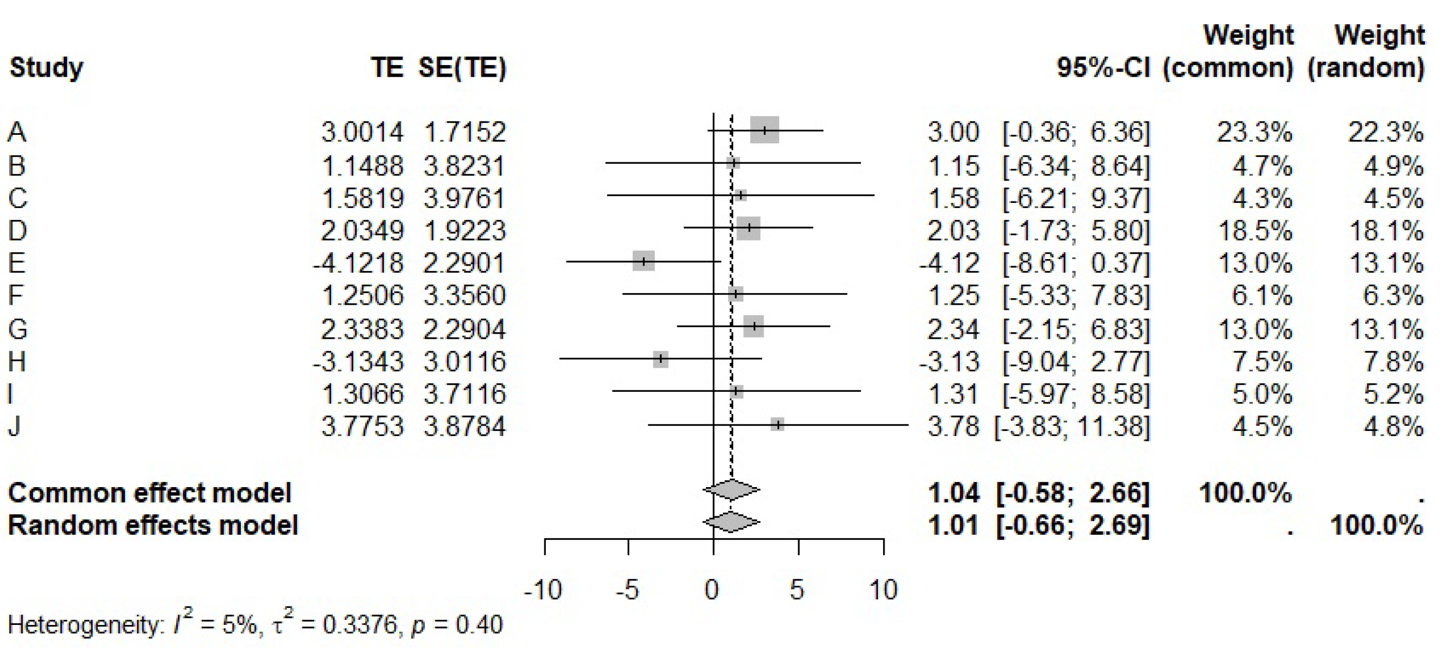
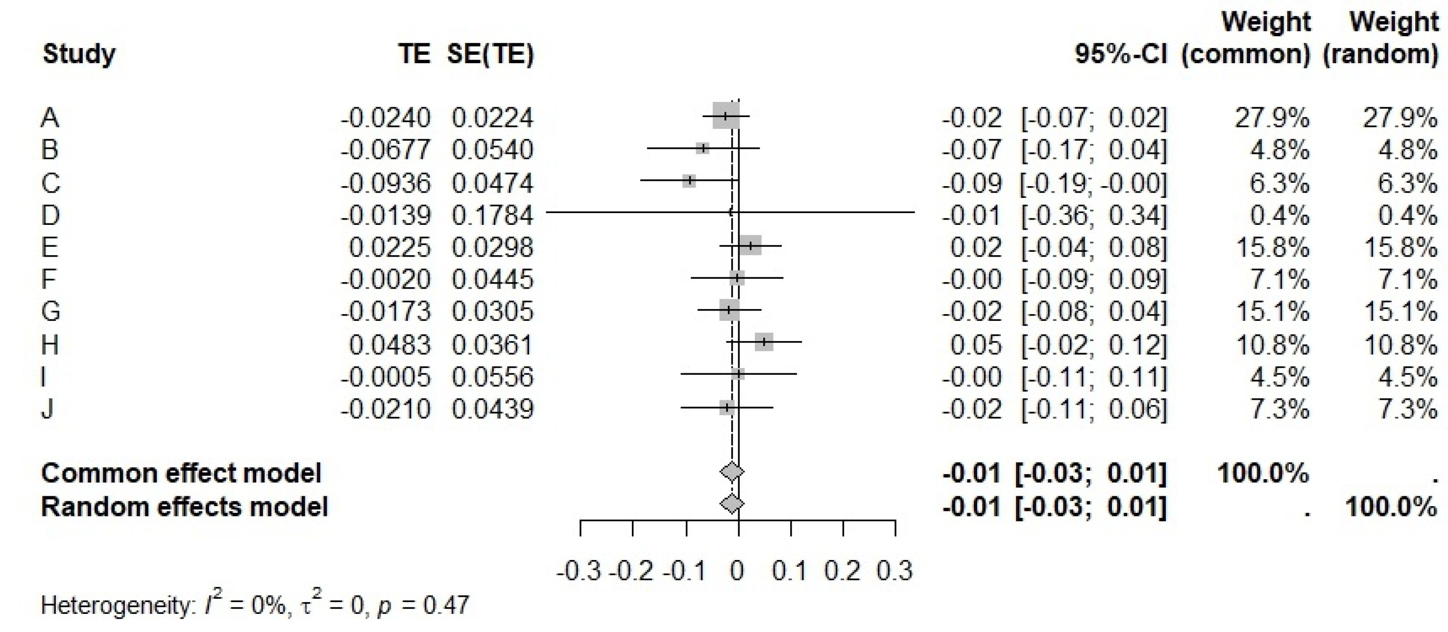
5. Example: Analyzing the 10 Cohort Studies in Table 1

5.1. Meta-Analysis for ${\beta }_1$

We wrote custom R functions to perform meta-analysis on the data in Table 1. The following R functions conduct both fixed-effect and random-effects meta-analyses for ${\beta }_1$.

studies <-read.csv(’https://raw.githubusercontent.com/enwuliu/

meta-analysis/main/random_effect_meta_sim.csv’, header = TRUE)

b1<-studies$b1  # beta1 from the 10 cohorts

var_b1 <- studies$var_b1  # variances of the coefficients

fixed_effect_meta <- function(B, V) {

  W <- 1 / V

  Beta <- sum(W * B) / sum(W)

  Var <- 1 / sum(W)

  resultlist <- list(’Overall beta’ = Beta, ’Overall variance’ = Var)

  return(resultlist)

}

random_effect_meta <- function(B, V) {

  W <- 1 / V

  Q <- sum(W * B^2) - (sum(W * B))^2 / sum(W)

  df <- length(B) - 1

  c <- sum(W) - sum(W^2) / sum(W)

  tau_square <- ifelse(Q > df, (Q - df) / c, 0)

  V_star <- V + tau_square

  W_star <- 1 / V_star

  Beta_star <- sum(W_star * B) / sum(W_star)

  Var_star <- 1 / sum(W_star)

  resultlist <- list(

 ’Overall beta’ = Beta_star,

 ’Overall variance’ = Var_star)

  return(resultlist)

}

fixed_b1 <- fixed_effect_meta(b1, var_b1)

fixed_b1

# $‘Overall beta‘

# [1] 1.040411

#

# $‘Overall variance‘

# [1] 0.6841809

random_b1 <- random_effect_meta(b1, var_b1)

random_b1

# $‘Overall beta‘

# [1] 1.014141

#

# $‘Overall variance‘

# [1] 0.7308388

From the results, the overall fixed-effect estimate for ${\beta }_1$ is 1.0404, with an overall variance of 0.6842. The overall random-effects estimate is 1.0141, with an overall variance of 0.7308.

The meta-analysis can also be conducted using the R package ‘meta’ [14], which can generate a forest plot (Figure 2) as follows:

library(meta)

b1.meta<- metagen(TE = b1,

         seTE = sqrt(var_b1),

         studlab = LETTERS[1:10],

         data = ,

         sm = "",

         method.tau = "DL",

         fixed = TRUE,

         random = TRUE,

         title = "Use R meta package")

summary(b1.meta)

forest(b1.meta)

# Review:  Use R meta package

#

# 95%-CI %W(common) %W(random)

# A  3.0014 [-0.3603;  6.3631]       23.3       22.3

# B  1.1488 [-6.3445;  8.6420]       4.7        4.9

# C  1.5819 [-6.2112;  9.3750]       4.3        4.5

# D  2.0349 [-1.7329;  5.8026]       18.5       18.1

# E  -4.1218 [-8.6104;  0.3668]       13.0       13.1

# F  1.2506 [-5.3271;  7.8282]       6.1        6.3

# G  2.3383 [-2.1507;  6.8274]       13.0       13.1

# H  -3.1343 [-9.0370;  2.7683]       7.5        7.8

# I  1.3066 [-5.9681;  8.5813]       5.0        5.2

# J  3.7753 [-3.8262; 11.3769]        4.5        4.8

#

# Number of studies: k = 10

#

# 95%-CI  z p-value

# Common effect model  1.0404 [-0.5808; 2.6616] 1.26  0.2085

# Random effects model 1.0141 [-0.6614; 2.6897] 1.19  0.2355

#

# Quantifying heterogeneity:

#   tau^2 = 0.3376 [0.0000; 15.2185]; tau = 0.5811 [0.0000; 3.9011]

# I^2 = 4.5% [0.0%; 64.1%]; H = 1.02 [1.00; 1.67]

#

# Test of heterogeneity:

#  Q d.f. p-value

# 9.42    9  0.3991

#

# Details on meta-analytical method:

#  - Inverse variance method

# - DerSimonian-Laird estimator for tau^2

# - Jackson method for confidence interval of tau^2 and tau

The results are the same as those obtained using our custom function, yielding an overall ${\widehat{\beta }}_1$=1.0404 for the common-effect model (fixed effect) and ${\widehat{\beta }}_1$=1.0141 for the random-effects model.

5.2. Meta-Analysis for ${\beta }_2$

We used the same R functions to perform meta-analysis for ${\beta }_2$:

b2 <- studies$b2  # beta2 from the 10 cohorts

var_b2 <- studies$var_b2  # variances of the coefficients

fixed_b2<-fixed_effect_meta(b2, var_b2)

fixed_b2

# $‘Overall beta‘

# [1] -0.01140614

#

# $‘Overall variance‘

# [1] 0.0001403961

random_b2<-random_effect_meta(b2, var_b2)

random_b2

# $‘Overall beta‘

# [1] -0.01140614

#

# $‘Overall variance‘

# [1] 0.0001403961

Both fixed-effect and random-effects meta-analyses yield an overall interaction effect of ${\beta }_2$ = −0.0114, with a variance of 0.0001404.

The meta-analysis can also be conducted using the R package ‘meta’, which can generate a forest plot (Figure 3) as follows:

# Review:     Use R meta package

#

# 95%-CI %W(common) %W(random)

# A -0.0240 [-0.0680;  0.0200]       27.9       27.9

# B -0.0677 [-0.1736;  0.0383]       4.8        4.8

# C -0.0936 [-0.1865; -0.0007]        6.3        6.3

# D -0.0139 [-0.3637;  0.3358]       0.4        0.4

# E  0.0225 [-0.0359;  0.0809]       15.8       15.8

# F -0.0020 [-0.0893;  0.0853]       7.1        7.1

# G -0.0173 [-0.0771;  0.0424]       15.1       15.1

# H  0.0483 [-0.0224;  0.1190]       10.8       10.8

# I -0.0005 [-0.1096;  0.1086]       4.5        4.5

# J -0.0210 [-0.1069;  0.0650]       7.3        7.3

#

# Number of studies: k = 10

#

# 95%-CI     z p-value

# Common effect model  -0.0114 [-0.0346; 0.0118] -0.96  0.3357

# Random effects model -0.0114 [-0.0346; 0.0118] -0.96  0.3357

#

# Quantifying heterogeneity:

#   tau^2 = 0 [0.0000; 0.0031]; tau = 0 [0.0000; 0.0558]

# I^2 = 0.0% [0.0%; 62.4%]; H = 1.00 [1.00; 1.63]

#

# Test of heterogeneity:

#   Q d.f. p-value

# 8.61    9  0.4742

#

# Details on meta-analytical method:

#   - Inverse variance method

# - DerSimonian-Laird estimator for tau^2

# - Jackson method for confidence interval of tau^2 and tau

5.3. Meta-Analysis for r

The following R functions were used to conduct a meta-analysis of the correlation coefficients.

fixed_effect_meta_r<-function(v1,v2,cov12,sample_size){

  r<-cov12/sqrt(v1*v2)                   #correlation coefficient

  z<-0.5*log((1+r)/(1-r))                #Fisher z transformation

  v<-1/(sample_size-3)                   #variance for z

  W<-1/v                                 #weight

  z_overall<-sum(W*z)/sum(W)             #overall random effect of z

  r_overall<-(exp(2*z_overall)-1)/(exp(2*z_overall)+1) #transform back to r

  return(r_overall)

}

random_effect_meta_r<-function(v1,v2,cov12,sample_size){

  r<-cov12/sqrt(v1*v2)                   #correlation coefficient

  z<-0.5*log((1+r)/(1-r))                #Fisher z transformation

  v<-1/(sample_size-3)                   #variance for z

  W<-1/v                                 #weight

  Q<-sum(W*z^2)-(sum(W*z))^2/sum(W)      #total variance or Q statistics

  c<-sum(W)-sum(W^2)/sum(W)              #c is the scaling factor

  df=length(v1)-1                        #degree of freedom

  tau_square<-ifelse(Q>df,(Q-df)/c,0)    #between study variance

$$$$

  v_star=v+tau_square

  W_star=1/v_star                        #new weight

  z_star<-sum(W_star*z)/sum(W_star)      #overall random effect of z

  r_overall<-(exp(2*z_star)-1)/(exp(2*z_star)+1) #transform back to r

  return(r_overall)

}

v1<-studies$var_b1

v2<-studies$var_b2

v12<-studies$cov_b1b2

sample_size<-studies$sample_size

r<-v12/sqrt(v1*v2)

fixed_meta_r<-fixed_effect_meta_r(v1,v2,v12,sample_size)

fixed_meta_r

#[1] -0.9600286

random_meta_r<-random_effect_meta_r(v1,v2,v12,sample_size)

random_meta_r

#[1] -0.9493409

The overall r for fixed-effect meta-analysis is −0.9600, while the random-effects meta-analysis gives −0.9493.

Similarly, meta-analysis on the correlation coefficient can be performed using the ‘meta’ package.

r<-v12/sqrt(v1*v2)

r.meta <- metacor(cor = r,

          n = sample_size,

          studlab = LETTERS[1:10],

          data = ,

          fixed = TRUE,

          random = TRUE,

          method.tau = "DL",

          hakn = FALSE,

          title = "Use R meta package")

summary(r.meta)

#

# Review:    Use R meta package

#

# COR          95%-CI %W(common) %W(random)

# A -0.8654 [-0.8722; -0.8583]        8.1       10.0

# B -0.9680 [-0.9687; -0.9673]        48.4       10.1

# C -0.9686 [-0.9698; -0.9674]        16.1       10.0

# D -0.9416 [-0.9455; -0.9374]        4.8       10.0

# E -0.9217 [-0.9281; -0.9149]        3.2       10.0

# F -0.9637 [-0.9656; -0.9616]        8.1       10.0

# G -0.9233 [-0.9319; -0.9136]        1.6        9.9

# H -0.9486 [-0.9528; -0.9441]        3.2       10.0

# I -0.9685 [-0.9725; -0.9639]        1.3        9.9

# J -0.9613 [-0.9639; -0.9586]        5.2       10.0

#

# Number of studies: k = 10

# Number of observations: o = 62000

#

# COR        95%-CI     z  p-value

# Common effect model  -0.9600 [-0.9606; -0.9594] -484.50        0

# Random effects model -0.9493 [-0.9631; -0.9306]  -22.01 < 0.0001

#

# Quantifying heterogeneity:

#  tau^2 = 0.0683 [0.0301; 0.2555]; tau = 0.2613 [0.1736; 0.5055]

# I^2 = 99.7%; H = 18.42

#

# Test of heterogeneity:

#  Q d.f. p-value

# 3052.41    9       0

#

# Details on meta-analytical method:

#   - Inverse variance method

# - DerSimonian-Laird estimator for tau^2

# - Jackson method for confidence interval of tau^2 and tau

# - Fisher’s z transformation of correlations

5.4. Overall Covariance for ${\beta }_1$ and ${\beta }_2$

Using Equation (13), the overall covariance is calculated as follows:

• Fixed-effect model

  $$\begin{array}{cc}\hfill cov{({\widehat{\beta }}_1,{\widehat{\beta }}_2)}_{fixed}& =r_{fixed}\times \sqrt{V_{fixed{\widehat{\beta }}_1}{V}_{fixed{\widehat{\beta }}_2}}\hfill \\ \hfill & =-0.9600286\times \sqrt{0.6841809\times 0.0001403961}\hfill \\ \hfill & =-0.009409082\hfill \\ \hfill \end{array}$$

  (24)
• Random-effects model

  $$\begin{array}{cc}\hfill cov{({\widehat{\beta }}_1,{\widehat{\beta }}_2)}_{random}& =r_{random}\times \sqrt{V_{random{\widehat{\beta }}_1}{V}_{random{\widehat{\beta }}_2}}\hfill \\ \hfill & =-0.9493409\times \sqrt{0.7308388\times 0.0001403961}\hfill \\ \hfill & =-0.009616357\hfill \\ \hfill \end{array}$$

  (25)

5.5. Calculating the Effect of Falls on Hip Fracture at Different Ages and 95% Confidence Intervals

Using the information derived above, we can calculate the effect of falls on hip fracture at different ages and their corresponding 95% confidence intervals using Equations (2) and (3). Additionally, we generate a plot of the rate ratio (RR) for hip fracture, comparing fallers versus non-fallers at various ages, by exponentiating the estimated $\beta$ coefficients.

To illustrate, we calculate the effect of falls on hip fracture for ages 50 to 90. First, we conduct a fixed-effect meta-analysis, followed by a random-effects meta-analysis.

The following R code calculates the interaction effect of falls with age and the corresponding 95% confidence intervals, using Equations (2) and (3), based on the results of the fixed- and random-effects meta-analyses.

library(ggplot2)

library(ggpubr)

plot_with_interaction <- function(age, b1, v1, b2, v2, r) {

cov_b1b2 <- r * sqrt(v1 * v2)

RR <- exp(b1 + b2 * age)

RR_lower <- exp((b1+b2*age)-1.96 * sqrt(v1+age^2 * v2+2 * age*cov_b1b2))

RR_upper <- exp((b1+b2*age)+1.96*sqrt(v1+age^2 * v2+2*age*cov_b1b2))

ndata <- as.data.frame(cbind(RR, RR_lower, RR_upper, age))

ggplot(data = ndata, aes(x = age)) +

geom_line(aes(y = RR)) +

geom_line(aes(y = RR_lower), color = "steelblue’’, linetype = ‘‘dashed’’) +

geom_line(aes(y = RR_upper), color = ‘‘steelblue’’, linetype = ‘‘dashed’’)+

scale_y_continuous(name = ‘‘Rate Ratio (RR): Fallers vs. Non-Fallers’’,

             limits = c(0, 4), expand = c(0, 0)) +

theme_bw() +

theme(axis.line = element_line(color = ’black’),

     axis.title.y = element_text(size = 8),

     axis.title.x = element_text(size = 8),

     axis.text.y = element_text(size = 8),

     axis.text.x = element_text(size = 8),

     plot.background = element_blank(),

     panel.grid.major = element_blank(),

     panel.grid.minor = element_blank(),

     panel.border = element_blank())

}

# Fixed-effect model

age <- seq(50, 90, 1)

b1 <- fixed_b1$‘Overall beta‘

v1 <- fixed_b1$‘Overall variance‘

b2 <- fixed_b2$‘Overall beta‘

v2 <- fixed_b2$‘Overall variance‘

r <- fixed_meta_r

p1 <- plot_with_interaction(age, b1, v1, b2, v2, r)

p1

# random-effects model

b1_rand <- random_b1$‘Overall beta‘

v1_rand <- random_b1$‘Overall variance‘

b2_rand <- random_b2$‘Overall beta‘

v2_rand <- random_b2$‘Overall variance‘

r_rand <- random_meta_r

p2 <- plot_with_interaction(age, b1_rand, v1_rand, b2_rand,

v2_rand, r_rand)

p2

p3 <- ggarrange(p1, p2,

         labels = c(‘‘A.Fixed Effect’’, ‘‘B.Random Effect’’),

         ncol = 2, nrow = 1)

p3

Figure 4 presents the hip fracture risk for fallers versus non-fallers at different ages, as determined by both fixed-effect (Figure 4A) and random-effects (Figure 4B) meta-analyses. For instance, in the fixed-effect meta-analysis, at 50 years old, the risk of hip fracture for fallers compared to non-fallers was HR = 1.6 (95 % CI: 0.88–2.92). The HR was calculated using Equation (2), where ${\widehat{\beta }}_1$= 1.0404 (overall fixed effect) and ${\widehat{\beta }}_2$ = −0.0114 (overall fixed effect). At age 50, the overall was calculated as $\beta$ = 1.0404 − 0.0114 × 50 = 0.4701, and exponentiating the value of $\beta$, the overall RR was $exp\left(0.4701\right)$ = 1.6.

The 95% confidence interval (CI) was computed using Equation (3). Since n is quite large, we approximated $t_{n-p-1,\alpha /2}$ as 1.96. The variance and covariance terms from the fixed-effect meta-analysis were as follows: var(${\widehat{\beta }}_1$) = 0.6848, var(${\widehat{\beta }}_2$) = 0.0001404, and cov(${\widehat{\beta }}_1$, ${\widehat{\beta }}_2$) = −0.009409 (from Equation (24)). Substituting these into Equation (3), the 95% CI was calculated as $0.4701\pm 1.96\times \sqrt{0.6848+{50}^2\times 0.0001404-2\times 50\times 0.009409}=(-0.1316,1.072)$. Exponentiating these limits gave the 95% CI for RR: 0.88 to 2.92. Similar calculations can be applied to obtain the RR and 95% CI for different ages, using both fixed-effect and random-effects meta-analyses.

From Figure 4, we observe that the risk ratio of hip fracture for fallers versus non-fallers decreases with increasing age. This suggests that interventions to prevent falls may be more effective when implemented earlier in life. However, readers should note that this analysis is for illustrative purposes only and is not intended to provide evidence on the relationship between falls and hip fractures.

6. Comparing the Results with the Multivariate Meta-Analysis

Multivariate meta-analysis can be used to analyze both main effects and interaction effects, as it enables the simultaneous synthesis of multiple effects [6,7,8]. Both R and STATA provide packages for conducting multivariate meta-analysis. In this study, we use the ‘mvmeta’ package [15] to perform a multivariate meta-analysis and compare its results with those obtained using our proposed methods.

library (mvmeta)

library (dplyr)

S <-as.matrix(select(studies, var_b1, cov_b1b2, var_b2))

model <- mvmeta (cbind ( studies$b1,studies $b2),S, method =‘‘ml’’)

summary(model)

# Call:  mvmeta(formula = cbind(studies$b1, studies$b2) ~ 1, S = S,

#method = ‘‘ml’’)

# Multivariate random-effects meta-analysis

# Dimension: 2

# Estimation method: ML

#

# Fixed-effects coefficients

# Estimate  Std. Error        z  Pr(>|z|)  95%ci.lb  95%ci.ub

# y1    1.1642      0.7770   1.4982    0.1341   -0.3588    2.6871

# y2   -0.0193      0.0128   -1.5060    0.1321   -0.0445    0.0058

# ---

#  Signif. codes:  0 ‘***’ 0.001 ‘**’ 0.01 ‘*’ 0.05 ‘.’ 0.1 ‘ ’ 1

#

# Between-study random-effects (co)variance components

# Structure: General positive-definite

# Std. Dev  Corr

# y1  0.8462  y1

# y2  0.0201  1

#

# Multivariate Cochran Q-test for heterogeneity:

#   Q = 77.9106 (df = 18), p-value = 0.0000

# I-square statistic = 76.9%

#

# 10 studies, 20 observations, 2 fixed and 3 random-effects parameters

# logLik    AIC    BIC

# -5.0854  20.1708  25.1495

$$$$

model$vcov

# y1.(Intercept) y2.(Intercept)

# y1.(Intercept)  0.603797649  -0.0058182353

# y2.(Intercept) -0.005818235   0.0001650336

b1_m<-model$coefficients[1,1]

b1_m

#[1] 1.164169

b2_m<-model$coefficients[1,2]

b2_m

#[1] -0.01934683

cov_m<-model$vcov[1,2]

cov_m

#[1] -0.005818235

The multivariate meta-analysis results yield ${\widehat{\beta }}_1$ = 1.1642 and ${\widehat{\beta }}_2$ = −0.0193, with var(${\widehat{\beta }}_1$)=0.6038, var(${\widehat{\beta }}_2$)=0.0001650 and covariance of $\mathrm{cov}({\widehat{\beta }}_1,{\widehat{\beta }}_2)$ = −0.005818. These values can be substituted into Equations (2) and (3) to calculate the 95% confidence intervals, which can then be compared with the results obtained using our method, as shown in Figure 5. It is evident that our method produces a narrower 95% confidence interval compared to the multivariate meta-analysis approach.

The following R code generates Figure 5.

plot_with_multivariate <- function(age, b1, v1, b2, v2, r,

b1_m, v1_m, b2_m,V2_m,cov_m) {

cov_b1b2 <- r * sqrt(v1 * v2)

RR <- exp(b1+b2 * age)

RR_lower<-exp((b1+b2*age)-1.96*sqrt(v1+age^2 * v2+2 * age*cov_b1b2))

RR_upper<-exp((b1+b2*age)+1.96 * sqrt(v1+age^2 * v2+2 *age*cov_b1b2))

RR_m <- exp(b1_m + b2_m * age)

RR_lower_m <-exp((b1_m+b2_m*age)-1.96 *sqrt(v1_m+age^2*v2_m+2 * age*cov_m))

RR_upper_m <-exp((b1_m+b2_m*age)+1.96 *sqrt(v1_m+age^2*v2_m+2 * age*cov_m))

ndata <- as.data.frame(cbind(RR,RR_lower,RR_upper,RR_m,RR_lower_m,RR_upper_m,age))

ggplot(data = ndata, aes(x = age)) +

geom_line(aes(y=RR,color=‘‘Correlation coefficient method’’)) +

geom_line(aes(y=RR_lower,color=‘‘Correlation coefficient method’’),

linetype=‘‘dashed’’)+

geom_line(aes(y=RR_upper,color=‘‘Correlation coefficient method’’),

linetype=‘‘dashed’’)+

geom_line(aes(y=RR_m,color=‘‘Multivariate meta-analysis’’)) +

geom_line(aes(y=RR_lower_m,color=‘‘Multivariate meta-analysis’’),

linetype =‘‘longdash’’)+

geom_line(aes(y=RR_upper_m,color=‘‘Multivariate meta-analysis’’),

linetype =‘‘longdash’’)+

scale_y_continuous(name = ‘‘Rate Ratio (RR): Fallers vs. Non-Fallers’’,

             limits = c(0, 5), expand = c(0, 0)) +

scale_color_manual(values = c(‘‘red’’, ‘‘blue’’))+

guides(color = guide_legend(title = ‘‘Methods’’))+

theme_bw() +

theme(axis.line = element_line(color = ’black’),

axis.title.y = element_text(size = 8),

axis.title.x = element_text(size = 8),

axis.text.y = element_text(size = 8),

axis.text.x = element_text(size = 8),

plot.background = element_blank(),

panel.grid.major = element_blank(),

panel.grid.minor = element_blank(),

panel.border = element_blank())

}

p4<-plot_with_multivariate(age, b1, v1, b2, v2, r,b1_m, v1_m, b2_m, v2_m, cov_m)

p4

7. An R Package for Calculating Overall Covariance in Meta-Analysis

To facilitate these calculations, we developed an R package called ’covmeta’, available on GitHub https://github.com/enwuliu/covmeta (accessed on 9 December 2024). This package can be installed and used within the R environment. Below is the R code to install the package and calculate the overall covariance using the data in Table 1:

#install the package

library(devtools)

install_github(‘‘enwuliu/covmeta’’)

$$$$

library(covmeta)

# Load the dataset

studies <- read.csv(’https://raw.githubusercontent.com/enwuliu/

meta-analysis/main/random_effect_meta_sim.csv’, header = TRUE)

$$$$

# Function arguments

b1 <- studies$b1      # Beta1 coefficients from the 10 cohorts

v1 <- studies$var_b1    # Variances of Beta1

b2 <- studies$b2      # Beta2 coefficients from the 10 cohorts

v2 <- studies$var_b2    # Variances of Beta2

cov_b1b2 <- studies$cov_b1b2  # Covariance between Beta1 and Beta2

sample_size <- studies$sample_size  # Sample sizes

# Calculate the overall main effect, interaction effect, and covariance

# Fixed-effect meta-analysis

cov_meta(b1, v1, b2, v2, cov_b1b2, sample_size, ’fixed’)

# random-effects meta-analysis

cov_meta(b1, v1, b2, v2, cov_b1b2, sample_size, ’random’)

8. Discussion

This paper proposes a method for calculating overall covariance for regression coefficients in the presence of interactions in a two-stage meta-analysis. The approach utilizes the statistical relationship between the correlation coefficient and variances to estimate the covariance. By conducting separate meta-analyses, the variances and correlation coefficient can be obtained. While statistical software packages provide built-in capabilities for analyzing the overall main effect, interaction effects, and their variances, merging covariances in meta-analysis when interactions are present remains a challenge [16]. We present a transparent and straightforward method to synthesize covariance in meta-analysis.

Detecting interactions is crucial in medical research, as interaction analyses can help determine whether an intervention is more effective for certain individuals [17,18,19]. In a two-stage meta-analysis, interactions between an exposure and covariates can be explored using meta-regression. However, the meta-regression method cannot study patient-level factors [20] and often suffers from low statistical power [21]. An alternative is dividing participants into subgroups (e.g., by age) and performing separate meta-analyses for each subgroup. While this avoids synthesizing interactions, it also tends to have low power [22].

Multivariate meta-analysis is another approach for investigating interactions in meta-analysis, allowing for the synthesis of correlated effects. For instance, in hypertension trials, systolic and diastolic blood pressure outcomes can be pooled using this approach [6,23]. In multivariate meta-analysis, the first-stage analysis estimates the coefficients (e.g., $\beta$ coefficients) and their covariances, which serve as inputs for the second-stage analysis conducted using mixed-model regression [8,24]. Compared to multivariate meta-analysis, our proposed method provides a narrower confidence interval for the overall effect.

Our method has some limitations. It assumes a linear relationship between the two regression coefficients, which may not always hold. Additionally, the estimation of the correlation coefficient may be less reliable and biased when the number of included studies is small [25]. Furthermore, this method is likely only useful for two-stage IPD meta-analysis. For one-stage approaches, particularly in advanced modeling contexts, covariance can be calculated directly from the regression modeling.

Meta-analysis has become a critical tool for synthesizing research findings across studies, enabling the identification of patterns and effect sizes in diverse fields. In future research in meta-analysis, particularly focusing on interaction effects and covariates, Bayesian hierarchical models can be developed to integrate interaction effects while accounting for study-level heterogeneity [26]. Traditional meta-regression models might be expanded to include individual level covariates as moderators, enabling the exploration of how study-level and participant-level covariates influence outcomes [27].

In conclusion, we have introduced a simple and transparent method for calculating covariance and confidence intervals in meta-analysis when interactions are present.

References

1. Vandenput, L.; Johansson, H.; McCloskey, E.V.; Liu, E.; Schini, M.; Åkesson, K.E.; Anderson, F.A.; Azagra, R.; Bager, C.L.; Beaudart, C.; et al. A meta-analysis of previous falls and subsequent fracture risk in cohort studies. Osteoporos Int. 2024, 35, 469–494. [Google Scholar] [CrossRef] [PubMed]
2. Kanis, J.A.; Johansson, H.; McCloskey, E.V.; Liu, E.; Åkesson, K.E.; Anderson, F.A.; Azagra, R.; Bager, C.L.; Beaudart, C.; Bischoff-Ferrari, H.A.; et al. Previous fracture and subsequent fracture risk: A meta-analysis to update FRAX. Osteoporos Int. 2023, 34, 2027–2045. [Google Scholar] [CrossRef] [PubMed]
3. Spineli, L.M.; Pandis, N. Two-stage vs. one-stage meta-analysis. Am. J. Orthod. Dentofac. Orthop. 2024, 166, 295–298. [Google Scholar] [CrossRef] [PubMed]
4. Riley, R.D.; Ensor, J.; Hattle, M. Two-stage or not two-stage? That is the question for IPD meta-analysis projects. Res. Synth. Methods 2023, 14, 903–910. [Google Scholar] [CrossRef] [PubMed]
5. Haller, B.; Mansmann, U.; Dobler, D.; Ulm, K.; Hapfelmeier, A. Confidence interval estimation for the changepoint of treatment stratification in the presence of a qualitative covariate-treatment interaction. Stat. Med. 2020, 39, 70–96. [Google Scholar] [CrossRef] [PubMed]
6. Hattle, M.; Burke, D.L.; Trikalinos, T.; Schmid, C.H.; Chen, Y.; Jackson, D.; Riley, R.D. Multivariate meta-analysis of multiple outcomes: Characteristics and predictors of borrowing of strength from Cochrane reviews. Syst. Rev. 2022, 11, 149. [Google Scholar] [CrossRef] [PubMed]
7. Basten, M.; van Tuijl, L.A.; Pan, K.Y.; Hoogendoorn, A.W.; Lamers, F.; Ranchor, A.V.; Dekker, J.; Frank, P.; Galenkamp, H.; Knol, M.J.; et al. Estimating additive interaction in two-stage individual participant data meta-analysis. Am. J. Epidemiol. 2024, kwae325. [Google Scholar] [CrossRef] [PubMed]
8. Sauerbrei, W.; Royston, P. Investigating treatment-effect modification by a continuous covariate in IPD meta-analysis: An approach using fractional polynomials. BMC Med. Res. Methodol. 2022, 22, 98. [Google Scholar] [CrossRef] [PubMed]
9. Khan, S. Meta-Analysis Methods for Health and Experimental Studies; Springer: Berlin/Heidelberg, Germany, 2020. [Google Scholar]
10. Borenstein, M.; Hedges, L.V.; Higgins, J.P.; Rothstein, H.R. Introduction to Meta-Analysis; John Wiley & Sons: Hoboken, NJ, USA, 2021. [Google Scholar]
11. Schwarzer, G.; James, R. Carpenter, Gerta Rucke. In Meta-Analysis with R; Springer: Berlin/Heidelberg, Germany, 2015. [Google Scholar]
12. Bakbergenuly, I.; Hoaglin, D.C.; Kulinskaya, E. Methods for estimating between-study variance and overall effect in meta-analysis of odds ratios. Res. Synth. Methods 2020, 11, 426–442. [Google Scholar] [CrossRef] [PubMed]
13. Dufour, J.-M. Covariance, Correlation and Linear Regression Between Random Variables. 2024. Available online: https://www2.cirano.qc.ca/~dufourj/Web_Site/ResE/ECON763_2024W/Dufour_2016_C_Covariances_W_Slides.pdf (accessed on 20 December 2024).
14. Schwarzer, G. Meta-Analysis in R. Systematic Reviews in Health Research: Meta-Analysis in Context; John Wiley & Sons: Hoboken, NJ, USA, 2022. [Google Scholar]
15. Chen, D.-G.D.; Peace, K.E. Multivariate Meta-Analysis. Applied Meta-Analysis with R and Stata; Chapman and Hall/CRC: Boca Raton, FL, USA, 2021. [Google Scholar]
16. Riley, R.D.; Debray, T.P.; Fisher, D.; Hattle, M.; Marlin, N.; Hoogl, J.; Gueyffier, F.; Staessen, J.A.; Wang, J.; Moons, K.G.; et al. Individual participant data meta-analysis to examine interactions between treatment effect and participant-level covariates: Statistical recommendations for conduct and planning. Stat. Med. 2020, 39, 2115–2137. [Google Scholar] [CrossRef] [PubMed]
17. Brankovic, M.; Kardys, I.; Steyerberg, E.W.; Lemeshow, S.; Markovic, M.; Rizopoulos, D.; Boersma, E. Understanding of interaction (subgroup) analysis in clinical trials. Eur. J. Clin. Investig. 2019, 49, e13145. [Google Scholar] [CrossRef] [PubMed]
18. Wang, X.; Piantadosi, S.; Le-Rademacher, J.; Mandrekar, S.J. Statistical Considerations for Subgroup Analyses. J. Thorac. Oncol. 2021, 16, 375–380. [Google Scholar] [CrossRef] [PubMed]
19. Richardson, M.; Garner, P.; Donegan, S. Interpretation of subgroup analyses in systematic reviews: A tutorial. Clin. Epidemiol. Glob. Health 2019, 7, 192–198. [Google Scholar] [CrossRef]
20. Higgins, J.P.T.; López-López, J.A.; Aloe, A.M. Meta-regression. In Handbook of Meta-Analysis; Chapman and Hall/CRC: Boca Raton, FL, USA, 2020; pp. 129–150. [Google Scholar]
21. Spineli, L.M.; Pandis, N. Problems and pitfalls in subgroup analysis and meta-regression. Am. J. Orthod. Dentofac. Orthop. 2020, 158, 901–904. [Google Scholar] [CrossRef] [PubMed]
22. Cuijpers, P.; Griffin, J.W.; Furukawa, T.A. The lack of statistical power of subgroup analyses in meta-analyses: A cautionary note. Epidemiol. Psychiatr. Sci. 2021, 30, e78. [Google Scholar] [CrossRef] [PubMed]
23. The Stata News, In the Spotlight: Multivariate Meta-Analysis. Available online: https://www.stata.com/stata-news/news37-1/multivariate-meta-analysis/ (accessed on 28 November 2024).
24. Riley, R.D.; Jackson, D.; White, I.R. Multivariate Meta-Analysis Using IPD. In Individual Participant Data Meta-Analysis: A Handbook for Healthcare Research; John Wiley & Sons: Hoboken, NJ, USA, 2021; pp. 311–346. [Google Scholar]
25. Stanley, T.D.; Doucouliagos, H.; Havranek, T. Meta-analyses of partial correlations are biased: Detection and solutions. Res. Synth. Methods 2024, 15, 313–325. [Google Scholar] [CrossRef] [PubMed]
26. Wu, D.; Goldfeld, K.S.; Petkova, E. Developing a Bayesian hierarchical model for a prospective individual patient data meta-analysis with continuous monitoring. BMC Med. Res. Methodol. 2023, 23, 25. [Google Scholar] [CrossRef] [PubMed]
27. Geissbühler, M.; Hincapié, C.A.; Aghlmandi, S.; Zwahlen, M.; Jüni, P.; da Costa, B.R. Most published meta-regression analyses based on aggregate data suffer from methodological pitfalls: A meta-epidemiological study. BMC Med. Res. Methodol. 2021, 21, 123. [Google Scholar] [CrossRef] [PubMed]
Figure 1. Schematic illustration of the meta-analytic framework.
Applsci 15 00141 g001
Figure 2. Forest plot for β ^ 1 .
Applsci 15 00141 g002
Figure 3. Forest plot for β ^ 2 .
Applsci 15 00141 g003
Figure 4. Effect of falls on hip fracture at different ages, comparing fallers vs. non-fallers.
Applsci 15 00141 g004
Figure 5. Comparison of correlation coefficient method and multivariate meta-analysis.
Applsci 15 00141 g005