The Wavelength Characteristics of Vertical Deformation and a Train Dynamics Simulation of Long-Span, Cable-Stayed Bridges Under Complex Loads

Abstract

Ballastless tracks have a high smoothness, but the corresponding laying requirements are strict. Therefore, the maximum span of cable-stayed bridges that can accommodate ballastless tracks is 392 m. For laying ballastless track structures over larger spans, the deformation characteristics of long-span, cable-stayed bridges under complex loads are incompletely understood, and the interaction between them and long-span track–bridge structures is unclear. The influence of the wavelength of the cosine wave on the track–bridge mapping of different orbital structures was explored. The wavelength characteristics of vertical deformation under complex loads were investigated. The track–bridge integrated model for the cable-stayed bridge was established to analyze the mapping relationship between the rail and the bridge and the wavelength characteristics of deformation. Based on the mapping relationships and the wavelength characteristics of deformation, the train–track–bridge dynamics simulation model was simplified. The results show that, when the minimum wavelength of bridge deformation surpassed 6 m, 10 m, and 16 m, the rail deformation in the ballasted track, the longitudinal-connected track, and the unit slab-type ballastless track accurately mirrored the deformation of the bridge. For the span of bridges ranging from 200 m to 600 m, the wavelength of vertical deformation ranged from 21 to 1270 m under complex loads. During local loads, the vertical deformation below the 200 m wavelength constituted a significant proportion near the pie. Considering the influence of the deformation on the train vibration response, the train–bridge dynamic coupling model can be employed to treat the track structure as a load to reduce the complexity of the model and enhance the calculation efficiency.

1. Introduction

The deformation of long-span, cable-stayed bridges experiences dynamic changes due to the combined effects of temperature, wind, train load, settlement, and creep during operation [1]. In China, extensive railway, cable-stayed bridges have main spans ranging from 200 m to over 1,000 m. As the main span increases, the stiffness of the cable-stayed bridge transitions from beam-dominated to cable-dominated [2,3,4]. This shift in stiffness significantly impacts the deformation of large-span, cable-stayed bridges, influencing the vibration acceleration of the car body. Therefore, a thorough investigation into the deformation characteristics of large-span, cable-stayed bridges under various loads is essential.

Some scholars have investigated the stiffness of long-span, cable-stayed bridges and girder–rail synergy. Chen et al. [5] systematically summarized the large-span, cable-stayed bridges of railroads constructed in China and put forward the recommended vertical deflection-to-span ratios for the large-span, cable-stayed bridges of railroads and public railways. Liu et al. [6] investigated the effects of structural parameters such as the number of side-span auxiliary piers, the side-to-center span ratio, and the main beam’s width-to-span ratio and height-to-span ratio on the stiffness and mechanical properties of cable-stayed bridges. Zheng et al. [7,8,9] explored the effect of elastic matting stiffness on the deformation of the main beams of large-span, railroad, cable-stayed bridges and the structural deformation of the interlayer of ballasted track slabs on the bridges and found that the uneven deformation of the interlayer between the track slabs and the base slabs could be better managed through the use of rubber matting. Taking a long-span, cable-stayed bridge with a span ranging from 300 m to 1000 m as the research object, Zhu et al. [10,11] established a refined, nonlinear model of large-span, cable-stayed bridge–ballastless track, analyzed the deformation characteristics of the long-span, cable-stayed bridge under the action of train load and temperature, and proposed that the measurement value of the mid-span chord, with a length of 60 m to 40 m, has a better match with the vertical vibration acceleration of the car body.

Based on the principle of the midpoint chord measurement method, Yang et al. [12,13] investigated the relationship between long-wave track irregularity and car body vertical acceleration in high-speed railroads and proposed the 60 m chord control standard of track irregularity under 250~350 km/h. Jin et al. [14] measured the track unevenness statistics of the different wavelength track unevenness and body acceleration relationship; the study shows that, at anything greater than a 200 m wavelength, the effect of the track irregularity on the train body acceleration is negligible. The correlation between track unevenness and vehicle vibration acceleration in the roadbed section was revealed by analyzing the track inspection data of the roadbed section. Some scholars [15,16], based on the Fourier transform analysis, investigated the multi-span, simply supported beam–bridge deformation wavelength decomposition and analyzed the bridge deformation and the wavelength characteristics of the correlation; the study shows that the 32 m wavelength deformation of the Xu-change (which is easily caused by high-speed trains) was coupled with the abnormal vibration of the bridge.

However, the actual number of large-span, railway, cable-stayed bridges in China is relatively small, and the feasibility study of long-span, cable-stayed bridges laying ballastless track is basically based on the idea that one bridge corresponds to one solution. The deformational characteristics of large-span, cable-stayed bridges and the mapping relationship between rail–bridge deformation under complex loads have not been systematically studied. It is difficult to determine the relationship between track irregularity and car body vibration acceleration on long-span, cable-stayed bridges. This paper investigates the wavelength characteristics and track–bridge deformation mapping of long-span, railway, cable-stayed bridges under complex loads. Additionally, the train dynamic simulation model has been simplified, enhancing the program simulation’s efficiency. Firstly, the finite element model of the rail structure to clarify the relationship between bridge deformation and rail deformation was established. Secondly, the structural arrangement scheme for a cable-stayed bridge with a main span ranging from 200 m to 600 m was designed. The deformation characteristic under complex loads was analyzed. Utilizing the research background of an actual long-span, cable-stayed bridge, we established an integrated model of the beam–rail system, examining the wavelength characteristics of vertical deformation and track–bridge deformation mapping on the cable-stayed bridge. Finally, the vehicle–rail–bridge dynamic coupling simulation model was simplified, based on the mapping relationship and wavelength characteristics.

2. Mapping Relationship Between Rail Deformation and Bridge Deformation

The track irregularity is classified by the length of the wave: the short wave, the medium wave, and the long wave. The long wave irregularity primarily stems from different foundational deformations, including the topographic relief, the roadbed settlement, and the bridge deformation. When scholars explore the correlation between the train vibration response and the track irregularity in the long-span bridge, it is crucial to initially establish the mapping relationship between the long-span bridge deformation and the track irregularity.

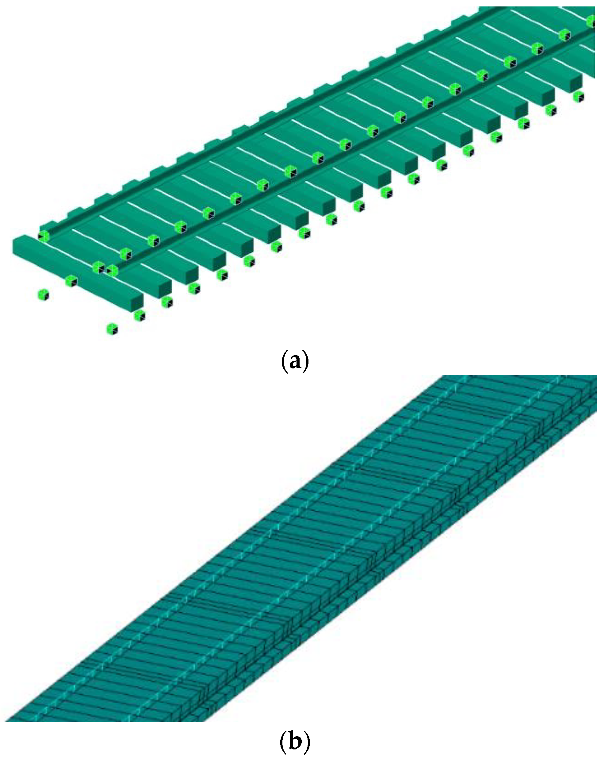
There are more types of the track structure used in China’s high-speed railway, mainly the ballasted track and the ballastless track. Ballastless tracks include the longitudinal ballastless track and the unit ballastless track. Finite element models of ballasted tracks, longitudinal ballastless tracks, and unit ballastless tracks were established by the ANSYS. The rail is modeled by the BEAM188 element. The fastener is simulated by a WJ-8-type fastener with the three-way spring element. The fastener is modelled with the COMBIN14 element in the vertical and transverse directions, and the COMBIN39 element in the longitudinal direction. The sleeper of the ballasted track is simulated by the BEAM188 element. The roadbed is simulated by the three-way spring element. For the ballastless track, the track slab and base slab are simulated using the SOLID 65 element. Their connection is modeled by the nonlinear spring element with the appropriate longitudinal, vertical, and lateral stiffness [17]. The finite element model is illustrated in Figure 1.

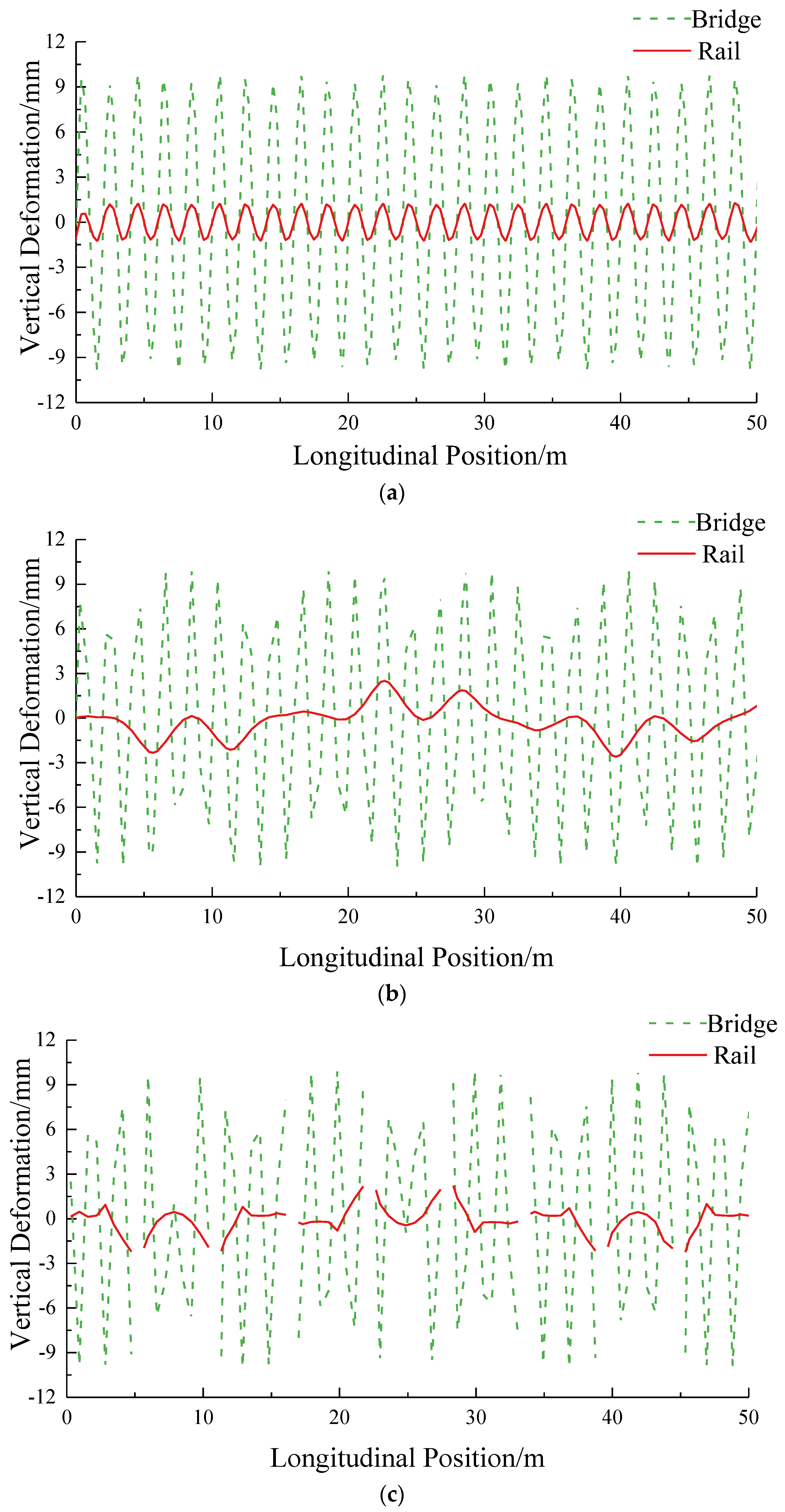
The deformation of the bridge can be analyzed by decomposing it into various wavelength deformations through the Fourier transform. To examined the difference between the rail deformation and the bridge deformation, continuous cosine waves with different wavelengths ranging from 0.5 m to 120 m are applied to the bottom of the track.

Figure 2 shows the difference between the rail deformation and the bridge deformation of the ballasted track (BT), the longitudinal-connected track (LT), and the unit slab-type ballastless track (USBT) influenced by continuous cosine waves with varying wavelengths. The figure reveals that, when the bridge deformation wavelength exceeds 6 m, 10 m, and 16 m for the BT, the LT, and the USBT, the difference in deformation between the bridge and the track is less than 1 mm. Conversely, for the wavelength of the bridge deformation below 6 m, 10 m, and 16 m, a substantial difference is observed in both track and bridge deformation.

Figure 3 shows the rail deformation and the bridge deformation under the cosine wave excitation of the 2 m wavelength. For the BT, LT, and USBT, their differences of the deformation, respectively, are 8.97 mm, 11.73 mm, and 11.27 mm.

For the BT, the LT, and the USBT, the 1:1 mapping relationship of the deformation between the rail and the bridge can be established when the bridge deformation, respectively, exceeds 6 m, 10 m, and 16 m. The rail deformation precisely mirrors the bridge deformation. However, when the bridge deformation wavelength is less than 6 m, 10 m, and 16 m, a significant difference in the deformation emerges between the track and the bridge. When the rail deformation cannot mirror the bridge deformation, it is necessary to establish a comprehensive rail–bridge model to accurately capture the rail deformation.

3. Wavelength Characteristics of Vertical Deformation of Long-Span, Cable-Stayed Bridges Under Complex Loads

We investigate the wavelength’s characteristics of the vertical deformation for long-span, cable-stayed bridges with a main span of 200 m to 600 m under complex loads. The process begins by establishing the structural parameters of cable-stayed bridges, focusing on designing large-span, cable-stayed bridges with main spans ranging from 200 m to 600 m. Then, vertical deformations of the bridge deck for these large-span, cable-stayed bridges are calculated, considering the impact of the cable-stayed-beam stiffness ratio under complex loads. Finally, employing the high-pass filtering theory, the vertical deformation of the bridge deck is decomposed. To obtain the range of vertical deformation’s wavelengths for long-span, cable-stayed bridges, the minimum and maximum wavelengths, representing 1% and 99% of the deformation energy, are extracted from the vertical deformation of the bridge.

3.1. Design of Long-Span, Cable-Stayed Bridges

After establishing the main beam’s span diameter, the primary step involves selecting the main beam material based on the span diameter. And the side span diameter, the bridge tower’s height, and the spacing of the cable-stay’s arrangement are provided. Furthermore, parameters such as the main beam’s cross-section, the cable’s diameter, and the tower’s cross-section are determined. In order to ensure the stiffness of the structure under complex loads, the design considers the vertical deflection of the main beam under train loads to keep it within the range of L/500.

Research suggests that cable-stayed bridges with a general main span of less than 400 m are best suited for the concrete main beam. In the case of main spans ranging from 400 m to 500 m, the choice involves comparing the composite beam and the concrete beam. For spans exceeding 500 m, it is recommended that we use the steel main beam or the composite beam. In this study, concrete main beams are considered for a main span of 200 m. For a main span of 400 m, both concrete beams and steel–concrete combination beams are contemplated. Additionally, a main span of 600 m is being considered for steel–concrete combination beams and steel main beams. Following the selection of the main span and the material of the main beam, the side span’s extent, the bridge tower’s height, and the spacing between the stay cables are determined based on the literature [18]. These values are detailed in

Table 1. Ratio of side span to main span diameter of double-tower cable-stayed bridges.

Type of Main Beam	Side Span/Main Span	Value
Steel Beam	0.30~0.40	0.35
Steel–Concrete Combination Beam	0.40~0.50	0.45
Concrete Beam	0.40~0.50	0.45

and

Table 2. Ratio of side span to main span diameter of double tower cable-stayed bridges.

Tower’s Height/Main Span	Value
0.2~0.33	0.27

.

In the investigation of the large-span, cable-stayed bridges ranging from 200 m to 600 m, the common design choice is the utilization of double-tower double-side cable-stayed bridges, employing the “H”-type concrete bridge tower. The cable-free zone near the bridge tower and abutment supports is set to a length of two to three times the diagonal cable spacing. These values are detailed in

Table 3. The distance between cables on the main beam and the bridge tower.

Type of Main Beam	Main Beam		Tower
	Value Range/m	Value/m	Value Range /m	Value/m
Steel Beam	8~15	12	2~5	3.5
Steel–Concrete Combination Beam	8~15	12	2~5	3.5
Concrete Beam	6~10	8	2~5	3.5

. To reduce the horizontal displacement at the mid-span of the main beam, strategically placed auxiliary piers are present at the side spans. The spanning ratio for a single auxiliary pier corresponding to the side spans is 4:6. And the ratio for double auxiliary piers corresponding to the side spans is 4:3:3. For the majority of cable-stayed bridges, a semi-floating system is employed, where dampers impose longitudinal shape constraints in the longitudinal direction. While these longitudinal dampers are active under seismic and wind loads, they have minimal impact on temperature-induced deformations. Consequently, no longitudinal restraints are introduced for the 200 m, 400 m, and 600 m cable-stayed bridges.

Fifteen structural schemes for cable-stayed bridges, considering different main beam’s types and auxiliary pier’s arrangements, are presented in

Table 4. Structural schemes of long-span, cable-stayed bridge with main span of 200~600 m.

Span of Main Beam/m			200			400						600
Deflection under move load/m			0.4			0.8						1.2
Material of main beam			Concrete beam			Concrete beam			Steel–concrete composite beam			Steel beam			Steel–concrete composite beam
Span of the side span/m			100			180			180			210			270
Height of the bridge tower/m			54			108			108			162			162
Spacing of cables/m	Main beam	The edge across the no-stay cable area	5			5			5			5			5
		Stay cables across side spans	8			7			10.5			8			10.7
		The non-stay cables of the bridge tower	15			19			15			15			15
		Stay cables in the main span	8			8			12			12			12
		The no-stay cable in the span	5			5			5			5			5
	Bridge tower		3.5			3.5			3.5			3.5			3.5
Height of the main beam/m			3.84			3.84						5.76
Width of bridge deck/m			14			14			14			18			18
Auxiliary span/m	First		0	0	30	0	0	54	0	0	54	0	0	63	0	0	80
	Second		0	40	30	0	72	54	0	72	54	0	84	63	0	108	80
	Third		100	60	40	180	108	72	180	108	72	210	126	84	270	162	110

. Finite element models of cable-stayed bridges are established by the Midas 2022 software. The main beam and bridge tower are modeled by the beam element. The cable is simulated by the truss element. The connection between the main beam and the support is modeled by the rigid arm unit. The support is rigidly connected with the foundation. The model of the long-span, cable-stayed bridge is depicted in Figure 4.

3.2. Vertical Deformation of Long-Span, Cable-Stayed Bridges Under Complex Loads

3.2.1. Complex Loads

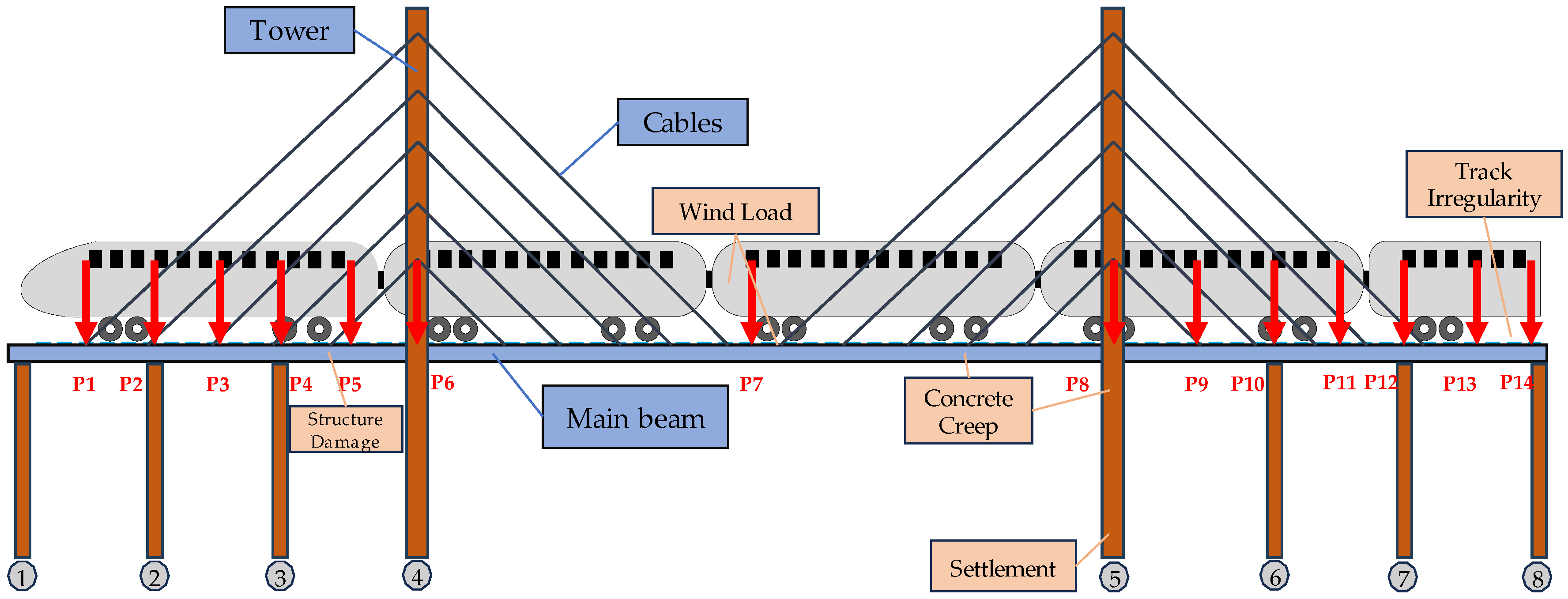
As shown in Figure 5, complex loads for long-span, cable-stayed bridges encompass train loads, the temperature, and the pier’s settlement, with the wind load’s effects currently excluded due to its minimal impact on vertical deformation. The vertical deformation and wavelength characteristics of cable-stayed bridges exhibit variations under different train formations. Train loads are considered for 8 cars with a length of 200 m and 16 cars with a length of 400 m. The temperature is factored in the overall lift of 20 °C and 15 °C of the cables. Considering the arrangement of piers, including the side pier’s settlement, the bridge tower’s settlement, the auxiliary pier’s settlement, and the settlement’s combinations, the settlement of piers is set at 5 mm. As an example, a seven-span steel–concrete combined beam cable-stayed bridge with a main span of 400 m is examined to investigate the distribution of vertical deformation under typical loads. P1 to P14 represent the moving load train working conditions corresponding to the first car acting on different positions of the bridge. Number ① to ⑧ represent the pier number.

3.2.2. Train Loads

Figure 6 illustrates the vertical deformation’s distribution of the cable-stayed bridge with the locomotive at different positions under the influence of eight trains. From the figure, the bridge’s deformation varies significantly as the train runs at different positions. When the train locomotive is on the middle span, the maximum deformation is 0.064 m near the middle span. As the locomotive moves to the right side, the maximum deformation position shifts to the right and continuously decreases. When the train runs on the left side span, the overall deformation of the bridge floor is relatively small. However, the deformation reverse bending points near the pier increase due to the presence of auxiliary piers.

Figure 7 shows the vertical deformation’s distribution of the cable-stayed bridge with the locomotive at different positions under the influence of 16 trains. The vertical deformation of the bridge floor increases overall when 16 vehicles are running on the cable-stayed bridge with a main span of 400 m. Since the length of the 16 trains is the same as the span of the main span of the bridge, the maximum deformation of the bridge floor is 0.097 m when the trains are fully deployed in the middle span. Compared with the 8-car formation, the vertical deformation waveform of the bridge deck is markedly different when the 16-car formation operates in the middle span and the right span.

3.2.3. Integral Temperature Rise and Fall

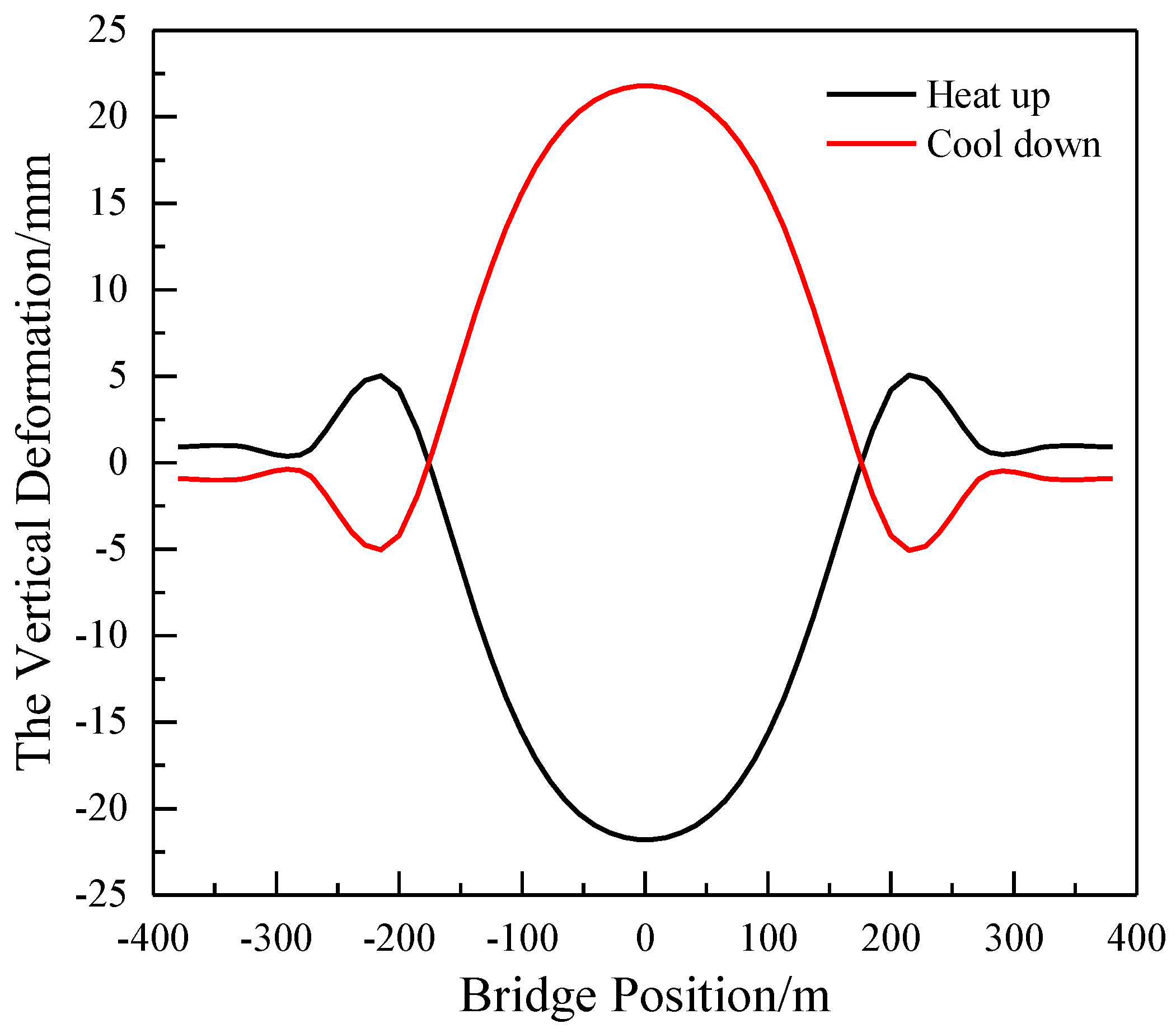
Given an overall temperature increase of 20 °C for the cable-stayed bridge, Figure 8 illustrates the vertical deformation of the main span 400 m cable-stayed bridge deck. The Figure 8 unveils dynamic changes in the bridge’s deformation corresponding to temperature fluctuations. The side span and the main span of the continuous beam bridge collectively exhibit upward arching during warming and downward deflection during cooling, with the larger vertical displacement in each span. The deformation waveform in the middle span demonstrates smoothness, while, in the side spans and near the supports of auxiliary spans, extremum points are evident, indicating the prevalence of short-wave deformations in these locations.

3.2.4. Difference Between the Cable’s Temperature and the Beam’s Temperature

Considering the temperature increase of 15 °C for cables, Figure 9 shows the vertical deformation of the cable-stayed bridge. From the figure, the maximum vertical deformation of bridge is 0.1 m under a temperature increase of 15 °C for cables. In comparison with the overall temperature difference, the temperature effect on the cable-stayed beam causes the more substantial vertical deformation of the bridge deck. The presence of auxiliary piers imposes constraints on the bridge deformation, leading to the more pronounced short-wave deformation in the side span under the influence of the temperature difference in the cable-stayed beam.

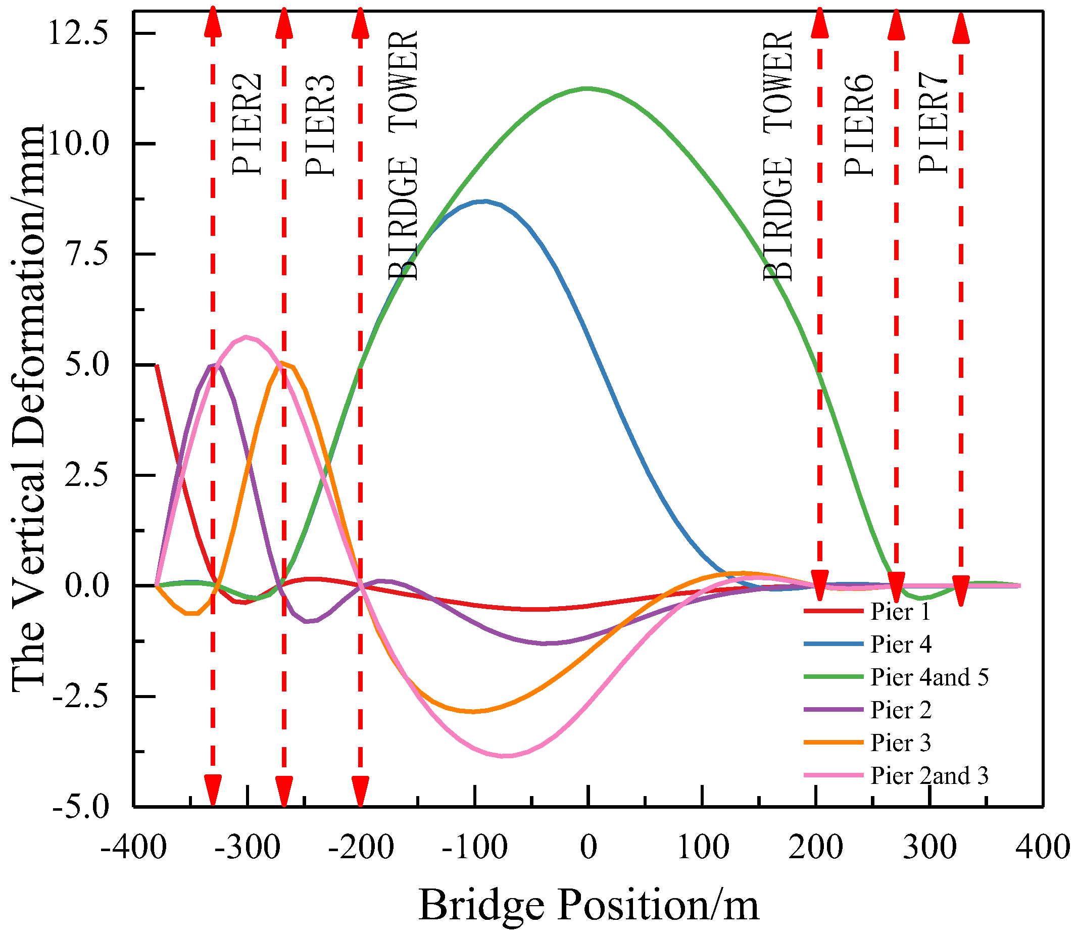
3.2.5. Settlement of Piers

The vertical deformation of the main beams in cable-stayed bridges displays significant variations under different forms of the pier’s settlement. Settlement scenarios, such as single-pier-assisted and multi-pier cross-settlement, prove to be less favorable for achieving long-wave smoothness in the track. When considering settlement conditions individually for side piers, auxiliary piers, and the tower, the vertical deformation of the main beam in the large-span, cable-stayed bridge is presented in the Figure 10. When the side span’s piers and auxiliary’s piers settle, the number of anti-bending points in the side span bridge deck increases, resulting in a more pronounced short-wave deformation. Conversely, when settlement occurs uniformly across all components, the overall smoothness of the bridge deck deformation improves.

3.3. Wavelength Range of Vertical Deformation of 200~600 m Cable-Stayed Bridge

The influence of the cable-stay stiffness ratio on the wavelength characteristic of vertical deformation in large-span, cable-stayed bridges under complex loads is examined. Two contrasting scenarios are explored: the strong beam and the weak cable, and the weak beam with the strong cable. To evaluate the vertical deformation under these conditions, adjustments are made to the diameter of the tension cables, resulting in cable-beam stiffness ratios of 100 and 0.001. The deformation of the long-span, cable-stayed bridge is a typical non-stationary signal. And the conventional signal decomposition method is difficult to use in effectively decomposing the long-wave deformation. Employing the Butterworth band-pass filtering principle, the vertical deformation is decomposed into wavelengths ranging from 25 m to 1200 m at intervals of 50 m. The minimum and maximum wavelengths are identified by intercepting those with 1% and 99% of the energy share in the bridge deformation. The resulting wavelength range of vertical deformation in long-span, cable-stayed bridges is presented in

Table 5. Minimum and maximum wavelengths of deformation of 200 m cable-stayed bridges.

The Span of the Main Span/m	Wavelength Type	Minimum Wavelength/m		Maximum Wavelength/m
	Cable-Beam Stiffness Ratio	0.001	100	0.001	100
200	Three-span	63.48	170.62	692.88	1268.29
	Five-span	31.74	151.37	756.29	1261.91
	Seven-span	21.38	122.31	599.79	1260.02
400	Three-span	38.64	304.22	1127.19	1268.81
	Five-span	28.57	266.57	1053.87	1263.92
	Seven-span	27.00	242.58	948.30	1262.22
600	Three-span	61.50	419.12	1237.67	1270.37
	Five-span	38.80	370.69	972.44	1270.74
	Seven-span	39.87	345.21	904.67	1270.12

.

From the table, it becomes apparent that, for the cable-stayed bridge sharing the same span arrangement, the stiffness of both the cable and the beam significantly influences the minimum and maximum wavelengths. Specifically, the weaker stiffness of the beam results in the minimum values for both minimum and maximum wavelengths, while the stronger stiffness of the beam leads to the maximum values. The substantial difference in the range of minimum and maximum wavelengths across these extremes underscores the profound impact of the cable-stayed beam stiffness on the linear wavelength characteristics of the cable-stayed bridge.

Furthermore, an increase in the number of auxiliary piers contributes to a gradual decrease in the minimum wavelength and the maximum wavelength. While the maximum wavelength remains relatively constant. For instance, in the case of a main span 200 m cable-stayed bridge, the minimum wavelength and the maximum wavelength are 21.38 m and 1268.29 m. In the case of a main span 400 m cable-stayed bridge, these values are 27 m and 1268.81 m. Finally, for a main span 600 m cable-stayed bridge, the minimum wavelength and the maximum wavelength are 38.8 m and 1270.74 m.

4. Deformation Mapping Relationship Between Long-Span, Cable-Stayed Bridge and Ballastless Track Based on Engineering

4.1. Engineering Introduction

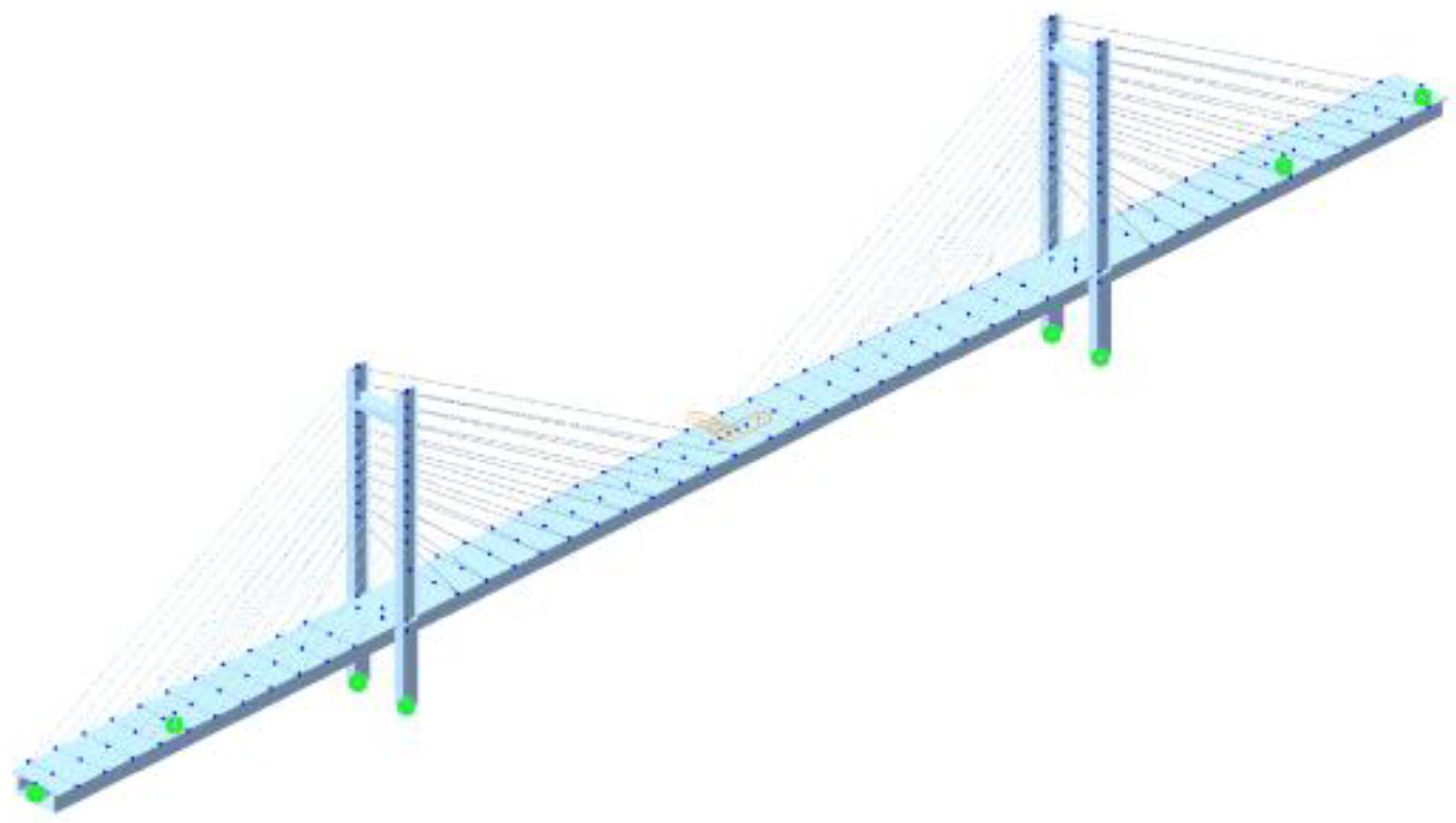
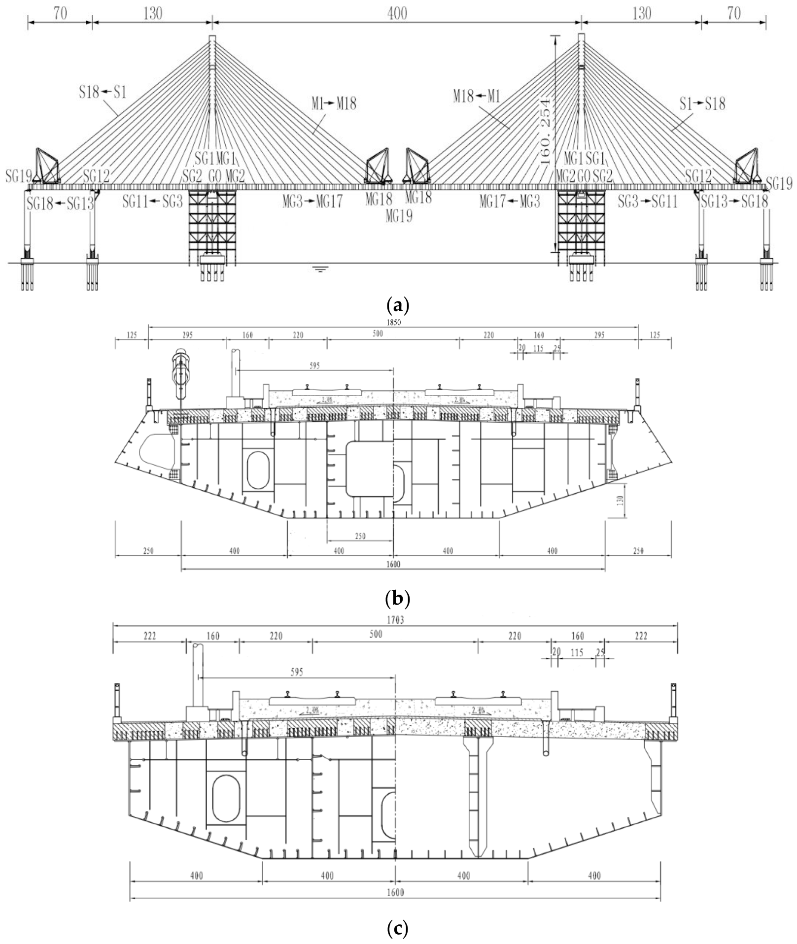
The sea-crossing bridge is a cable-stayed bridge with the 400 m length of the main span. Illustrated in Figure 11, the bridge adopts a semi-floating system and adheres to a span arrangement of (70 + 130 + 400 + 130 + 70) m. The main beam, fashioned from a steel–concrete combination, maintains the 10.5 m length of the standard section. The tower’s design follows the H-type configuration. And the height of the bridge tower is 3.649 times the width of the main beam. Cables adopt a fan-shaped layout, totaling 72 pairs. Engineered for a speed of 350 km/h and featuring a two-lane configuration, the main line spacing is fixed at the 5 m. The bridge integrates a ballastless track structure, laying a seamless line.

4.2. Finite Element Model of Long-Span, Cable-Stayed Bridge and Ballastless Track

The long-span, cable-stayed bridge employs the multi-degree-of-freedom finite element method to establish the finite element model of the long-span, cable-stayed bridge and the ballastless track, as shown in Figure 12.

The CRTS III-type plate ballastless track consists of the rail, the fastener, the track plate, the self-compacting concrete, the isolation layer, and the base plate. To capture the complexity of the bridge model, the cable is simulated using the link element, and the rest of the structure is represented by the beam element. The rigid connection is introduced to model the connection between the main beam and the pier. The rail is simulated using beam elements, while the track plate and the base plate are represented by solid elements, while the isolation layer and the fastener are depicted using three-way spring elements. To address the continuous deformation of the rail at the beam end position, three span bridges of the 32 m simply supported beam are established, following the side pier of the large-span, cable-stayed bridge.

4.3. Characteristics of Deformation Wavelength of Long-Span, Cable-Stayed Bridges

As the train traverses the bridge and the auxiliary pier settles, the vertical deformation of the expansive cable-stayed structure becomes more pronounced within the wavelength range of less than 200 m. Moreover, the temperature differential between the cables and beams significantly impacts the vertical deformation of the main span. Considering these factors, a thorough examination is undertaken to explore the wavelength characteristics of vertical deformation in a long-span, cable-stayed bridge. This investigation focuses specifically on scenarios involving the 5 mm settlement of auxiliary piers and a 15 °C temperature rise in tension cables, particularly during the train’s entry onto the bridge.

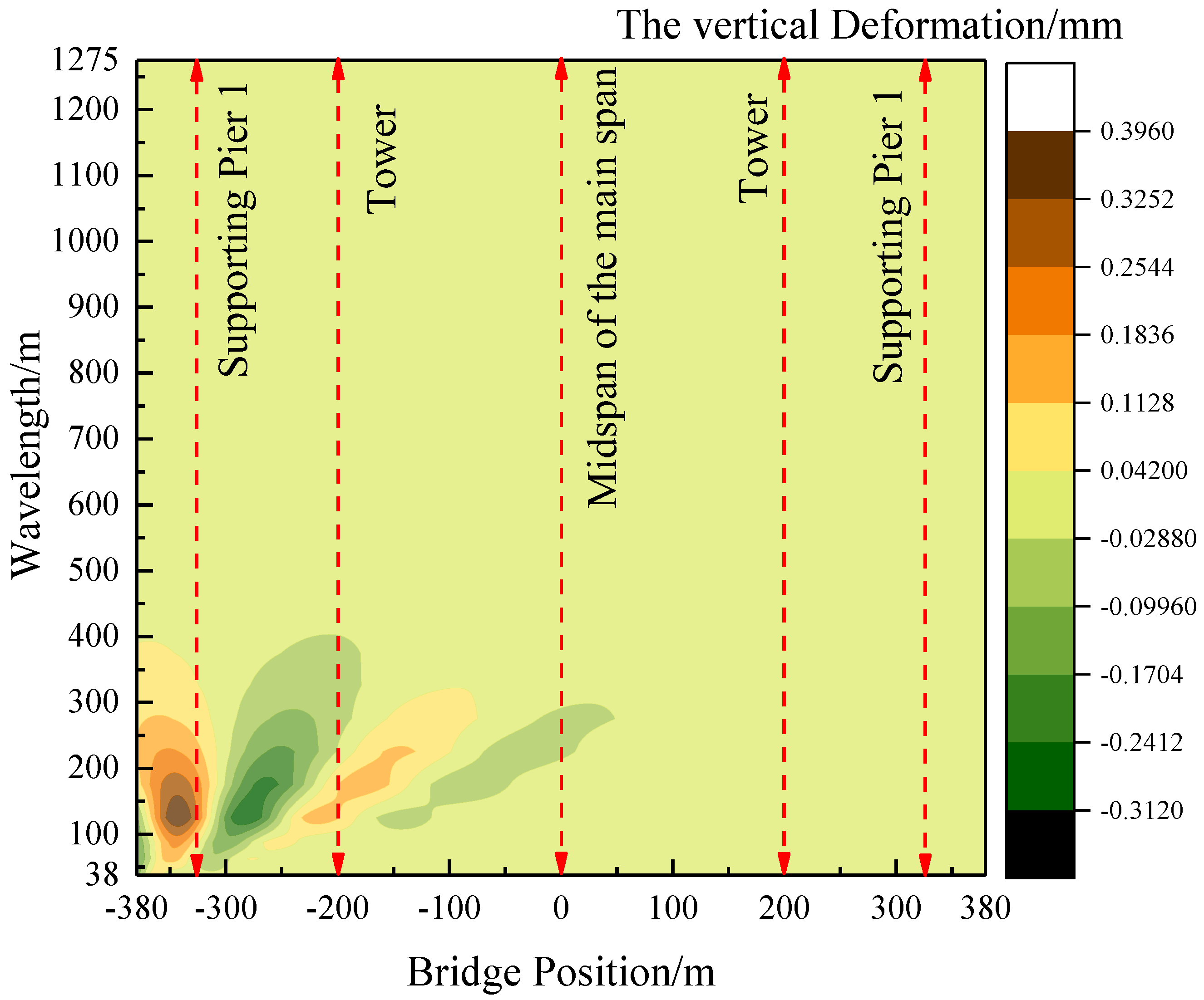
In Figure 13, the distribution of vertical deformation in each wavelength section at different locations of the long-span, cable-stayed bridge during the train’s entry is depicted. As the train approaches the bridge, noticeable variations in the deformation wavelength characteristics emerge, particularly affecting the vertical deformation of the left span. Generally, the right span bears the predominant vertical deformation of the long-span, cable-stayed bridge. The auxiliary span, on the other hand, predominantly undergoes deformation in wavelengths below 200 m, with larger deformation values. Notably, the deformation cutoff wavelength in the auxiliary span is set at 400 m.

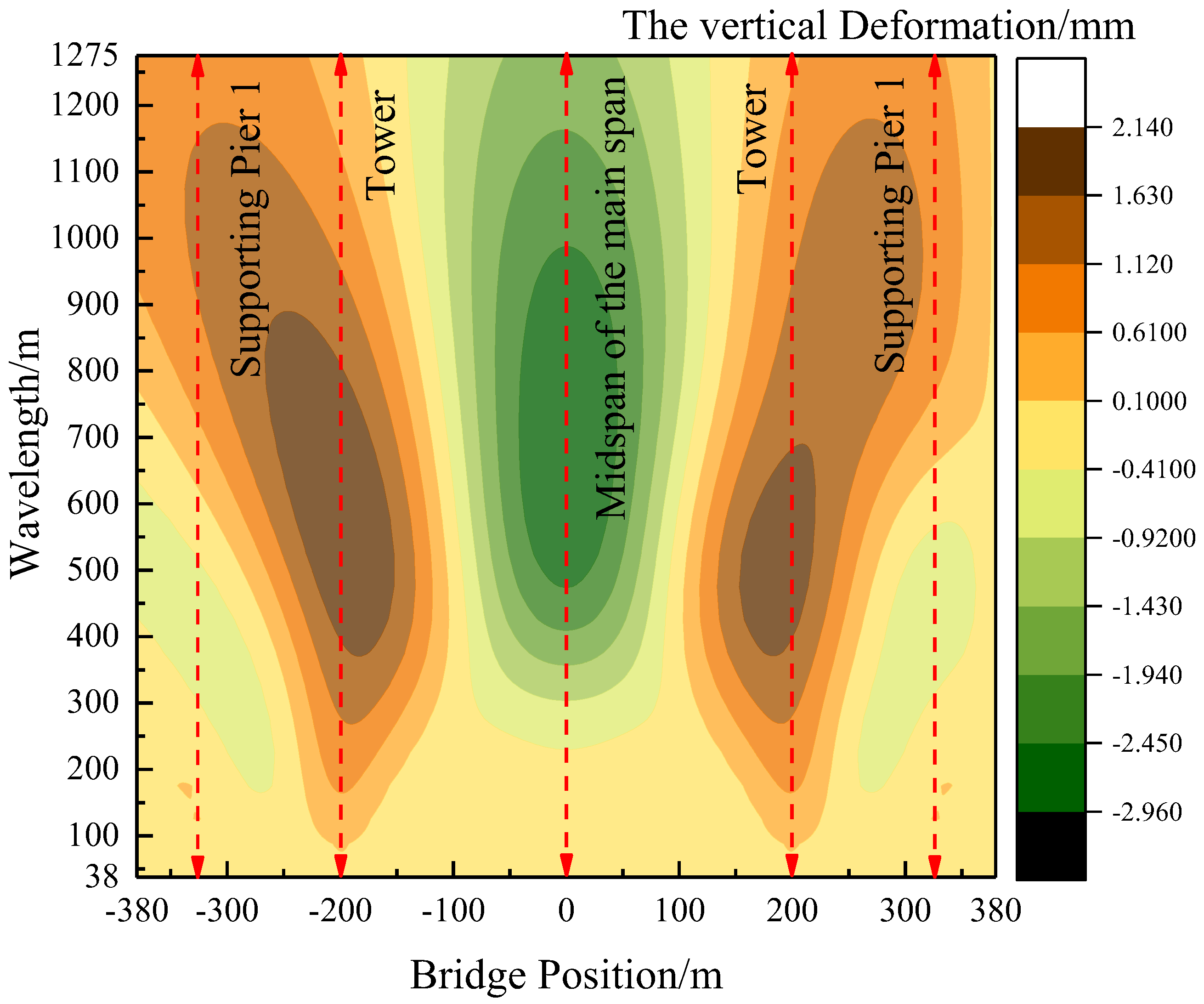
Figure 14 illustrates the distribution of vertical deformation in each wavelength section at different locations of the long-span, cable-stayed bridge during the warming up of cables. The figure highlights a downward deflection in the main span and an upward arching in the side spans. In the wavelength section below 200 m, it is evident that the vertical deformation is more pronounced at the location of the bridge tower. This suggests that the long-wave smoothness of the bridge tower, under the influence of the warming up of cables, is relatively poor compared to other locations. The side span and mid-span locations are primarily dominated by long waves exceeding 200 m, with deformation concentrated in the wavelength range of 400~1000 m.

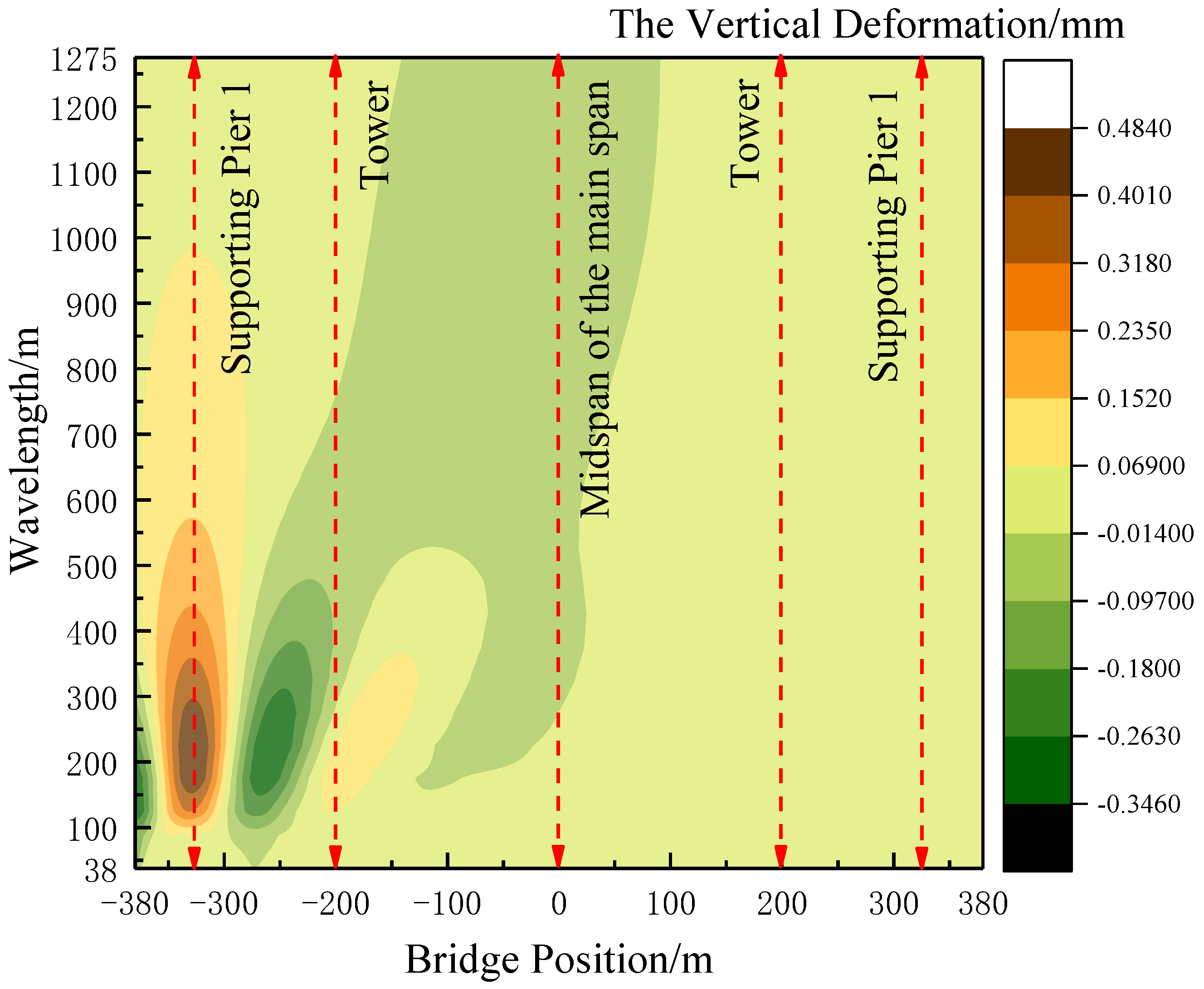
In Figure 15, the vertical deformation distribution of each wavelength section at different locations of the long-span, cable-stayed bridge is depicted when a settlement of 5 mm occurs in the left auxiliary pier. The figure illustrates that, when the auxiliary piers settle, the vertical deformation primarily occurs at the location of the left side span and the left tower. Specifically, the vertical deformation of the left side span is concentrated in the 100~450 m wavelength section, with the maximum value of the wavelength decomposition deformation occurring around 200 m. Notably, the settlement of auxiliary piers has a lesser impact on the deformation at the bridge tower position.

4.4. The Mapping Relationship Between Long-Span, Cable-Stayed Bridge and Track Deformation

4.4.1. Temperature Difference Between Cable and Beam

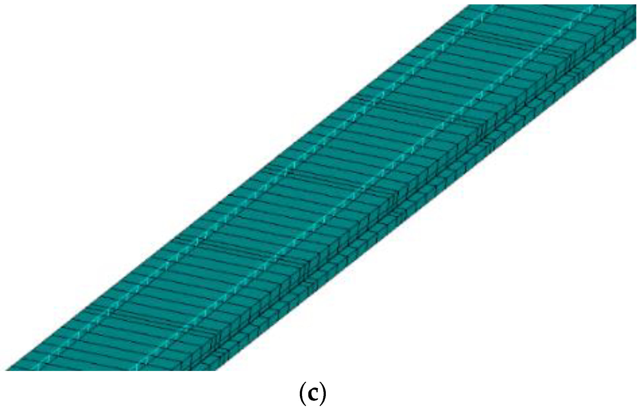
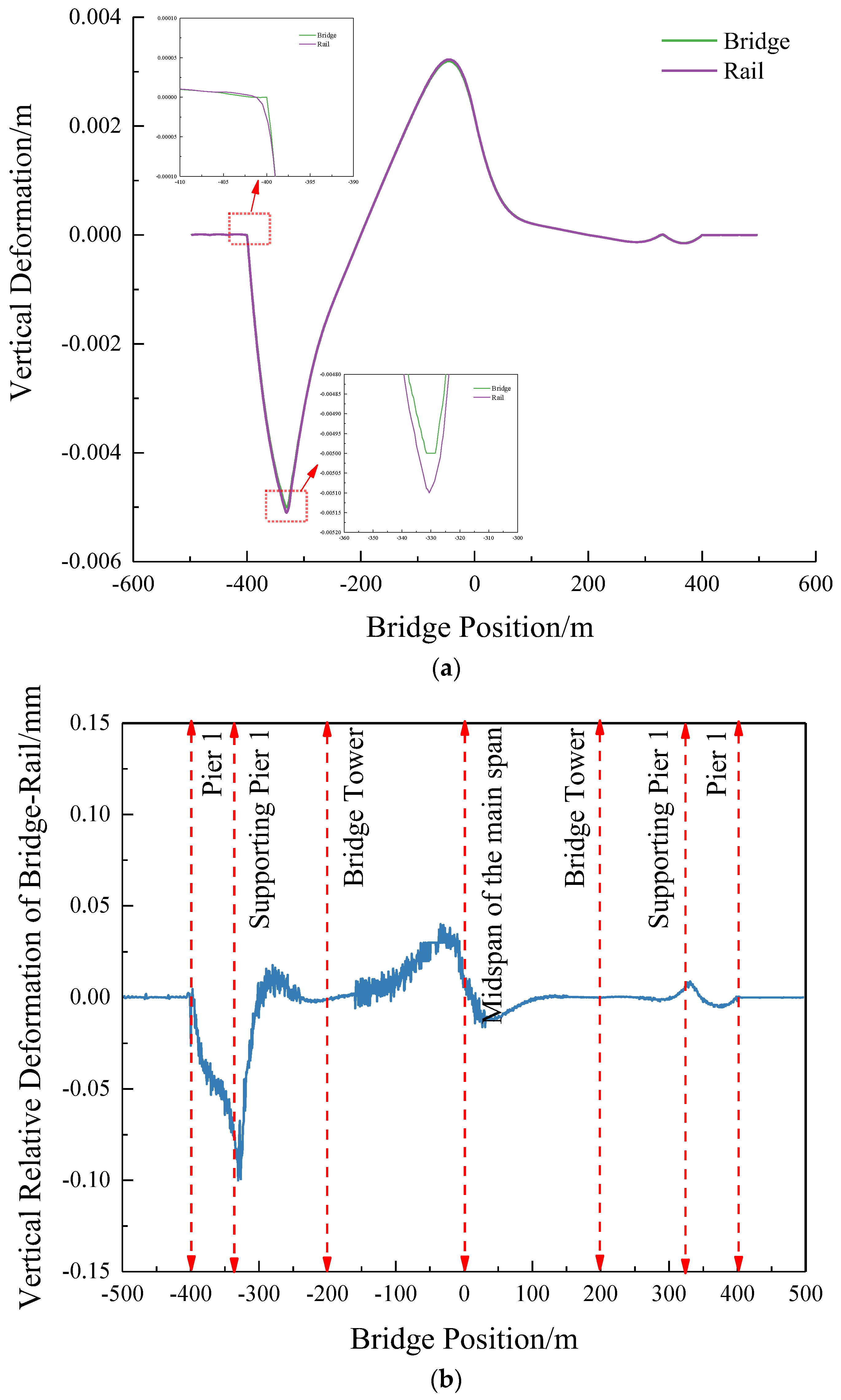
The impact of the temperature’s difference between the main beam and the cable on the vertical deformation of large-span, cable-stayed bridges is notably significant. Figure 16 illustrates the mapping relationship of the vertical deformation between the bridge and the track under the condition of a 15 °C warming of the cable-stayed cables.

From the figure, the maximum vertical deformation occurs at the midpoint of the main span when the cable-stayed cables are warmed, and there is a noticeable folding angle observed near the bridge tower. Upon comparing the vertical deformation of the rail surface with that of the bridge, a slight deviation is evident between the main span and the bridge tower, measuring less than 1 mm. The deformation in the rest of the positions remains relatively consistent. This observation suggests that the vertical deformation of the rail surface under the influence of the temperature difference in the cable-stayed beam is essentially consistent with the deformation of the cable-stayed bridge.

4.4.2. Settlement of Auxiliar Pier

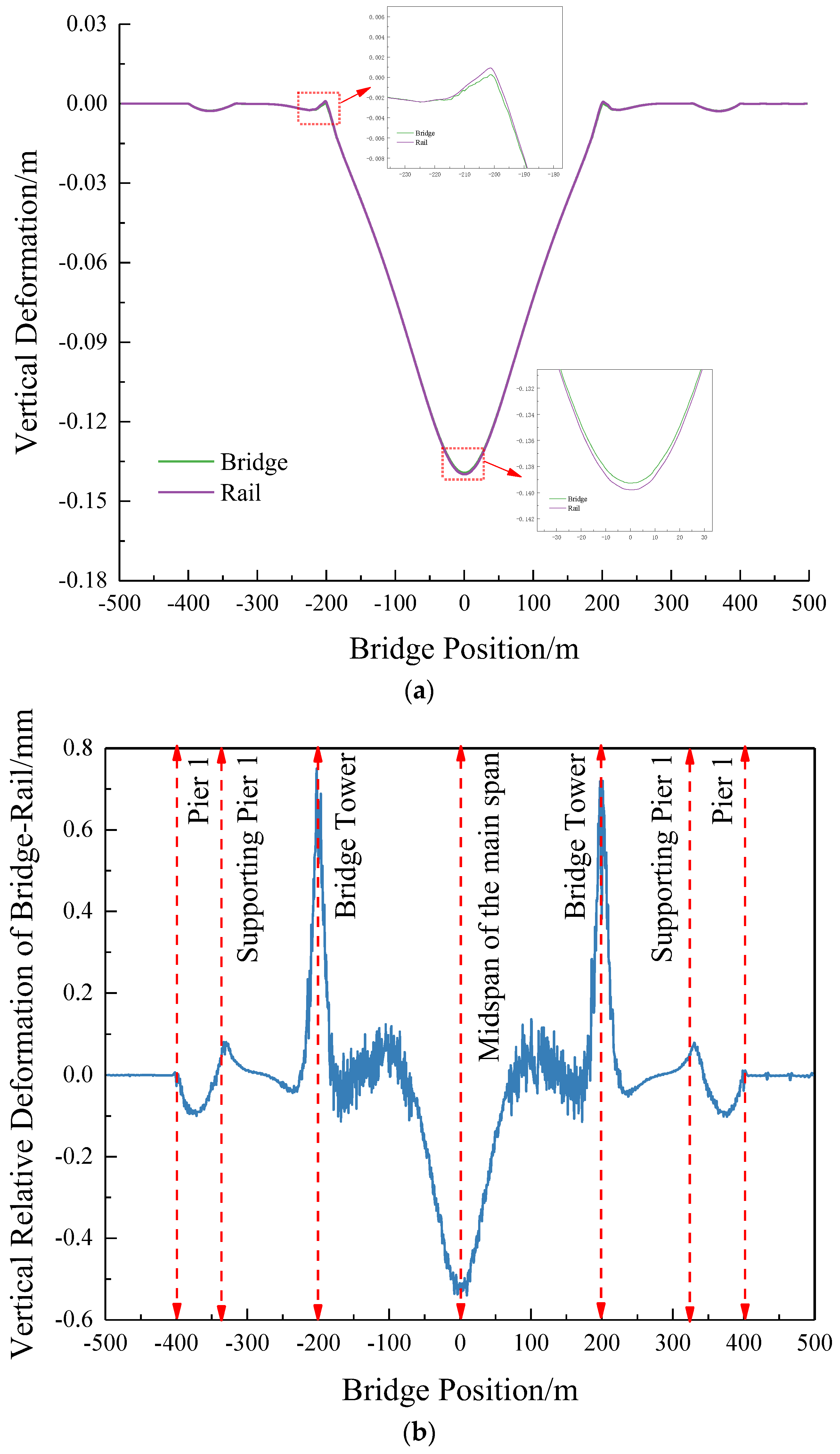
For the subsidiary pier settlement of less than 200 m in long-span, cable-stayed bridges, a significant proportion is attributed to short-wave deformations. The mapping relationship between the track deformation and the bridge deformation is examined by considering the 5mm settlement of the left span auxiliary pier, as depicted in Figure 17.

From the figure, it is apparent that, when the auxiliary pier settles at 5 mm, folding corners become evident at the beam ends, auxiliary piers, and the mid-span location of the main span. While there is a slight deviation between the track surface deformation and the bridge deck deformation at this location, impacting smoothness, overall, the two deformations remain relatively consistent. This suggests that when the auxiliary pier settles at 5 mm, the vertical deformation of the rail surface aligns closely with the deformation of the cable-stayed bridge.

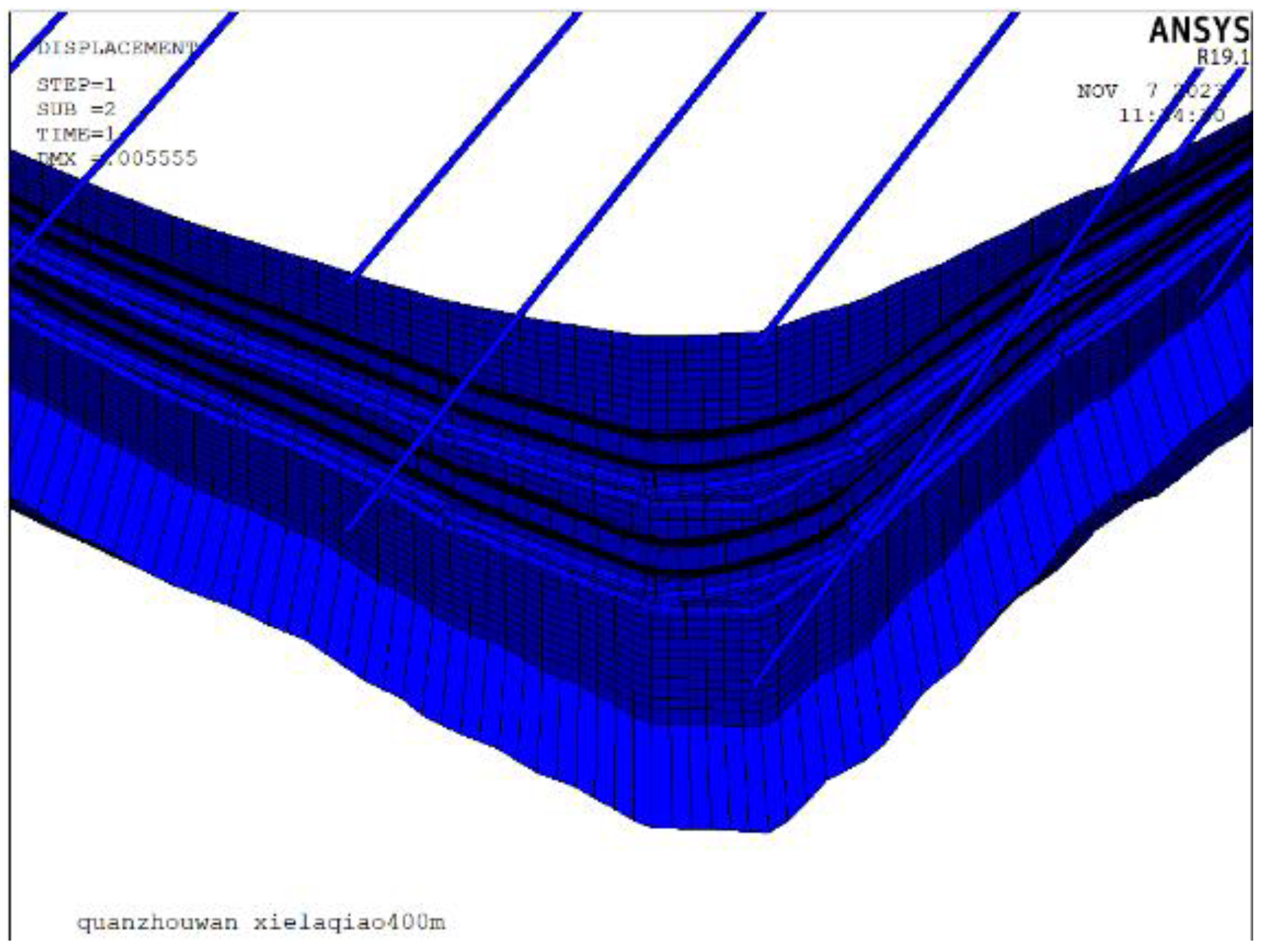
In Figure 18, the cloud picture of the bridge deck deformation and track deformation at the settlement location of the auxiliary pier is presented. The figure indicates a more pronounced vertical folding angle at the location of the auxiliary pier settlement. Notably, there is an evident difference in the deformation between the track plate and the base plate. Based on these observations, it is advisable to focus on the conditions of the track service, especially at locations where there is a sudden change in abutment and other kinds of stiffness during the operational period.

5. Simplification of Train Dynamic Simulation Model Based on Deformation Wavelength Characteristics of Long-Span, Cable-Stayed Bridges

5.1. Overview

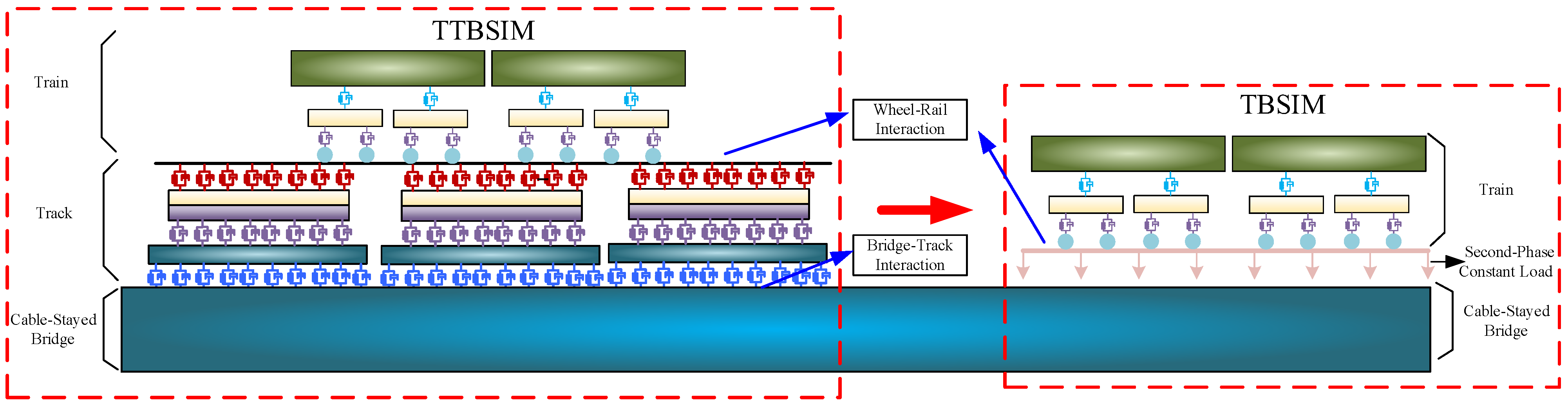
At present, most scholars have explored the effect of the vertical deformation of the long-span, cable-stayed bridge on the car body vibration response by establishing the train–track–bridge dynamic coupling simulation model. Although the dynamic response of the bridge deformation to the train can be analyzed through the train–track–bridge dynamic simulation, considering the large span of long-span bridge and the small load step of the dynamic simulation calculation program, it is difficult to complete the research on the response of the bridge’s deformation to the train vibration under complex loads. Considering the track structure, the computational efficiency of the dynamic simulation is reduced, and the complexity of the train–bridge dynamic simulation model is increased. According to the analysis of the upper section, the vertical deformation of the long-span, cable-stayed bridge can be mapped to the rail’s deformation under complex loads. And the rail can completely follow the deformation of the long-span, cable-stayed bridge floor. Therefore, the train–track–bridge dynamic coupling simulation theory can be simplified. And the track structure can be simplified as a constant load. The train–bridge dynamic coupling simulation model is used to calculate the vehicle vibration response when the train passes the long-span, cable-stayed bridge.

The accuracy of the train–large-span, cable-stayed bridge dynamic simulation model is verified under conditions of the random irregularity, the tension cable heating in long-span, cable-stayed bridges, and the auxiliary pier’s settlement deformation. This verification is conducted by comparing the vehicle vibration response calculated using the TTBSIM model and the TBSIM model.

5.2. Train Dynamic Response Simulation Model

5.2.1. Train–Track–Bridge Dynamic Coupling Model

In the dynamic coupling simulation model for the train–rail–bridge system, the two-system suspension multi-rigid body model with a total of 35 degrees of freedom is selected for the vehicle. The parameters of the vehicle model are sourced from the literature [19]. The track model and the bridge model are implemented using the method of the discrete finite element for the finite element calculation, as shown in Figure 19.

The train–track relationship is determined by the wheel–rail contact geometry and the resulting the interaction force [20,21]. The wheel–rail contact geometry is computed using the trace method, and Hertz’s nonlinear elastic contact theory is applied for calculating the wheel–rail normal force. Longitudinal, transverse, and spin creep-slip forces between wheel tracks are initially solved using Kalker’s nonlinear modified creep theory.

The interaction relationship between the track and the bridge is determined based on the action node’s numbers of the track structure and bridge structure. The numerical interpolation is employed to calculate the track–bridge interaction force and the displacement. The vibration equation of the coupled dynamic model for the train–rail–bridge system are solved using the Newmark-β method, with the displacement convergence threshold set at 10⁻⁷ m [22].

5.2.2. Train–Bridge Dynamic Coupling Model

In the train–bridge dynamic coupling simulation model, the consideration of the track structure parametric vibration effects is omitted. Instead, the track structure is simplified and applied to the bridge main beam as a second-phase constant load, as shown in Figure 19.

The wheel–rail contact model in the train–bridge system utilizes a faster method for the wheel–rail close-fitting model [23], and the creep-slip force between the wheel and the rail is initially determined based on Kalker’s nonlinear correction creep-slip theory. For the vehicle, the two-system suspension multi-rigid body model with a total of 23 degrees of the freedom is selected. The bridge model employs the method of the discrete finite element to establish the finite element model. The vibration equation of the coupled dynamic model for the train–bridge system and the displacement convergence conditions are adopted from the train–track–bridge dynamic coupling model.

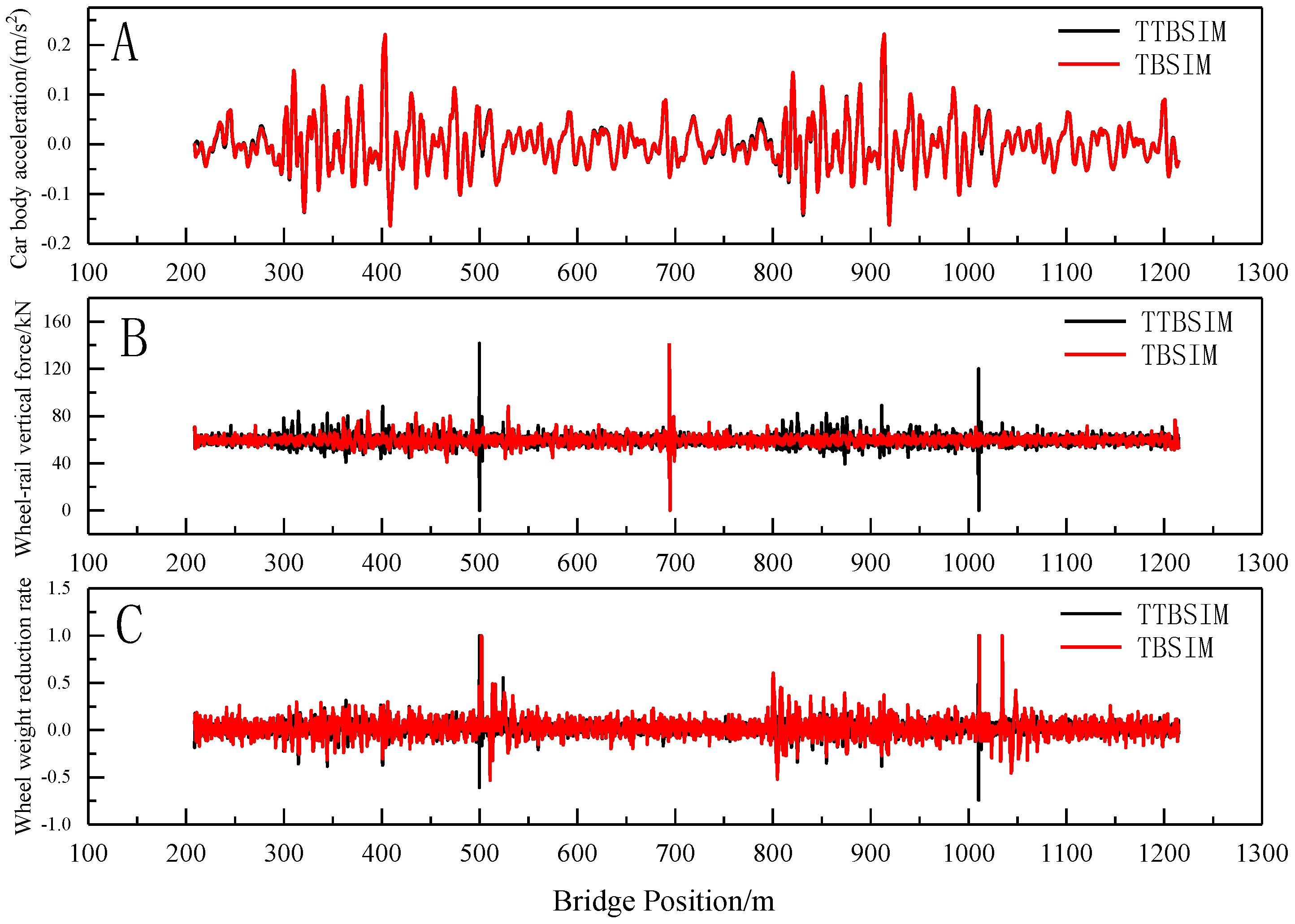
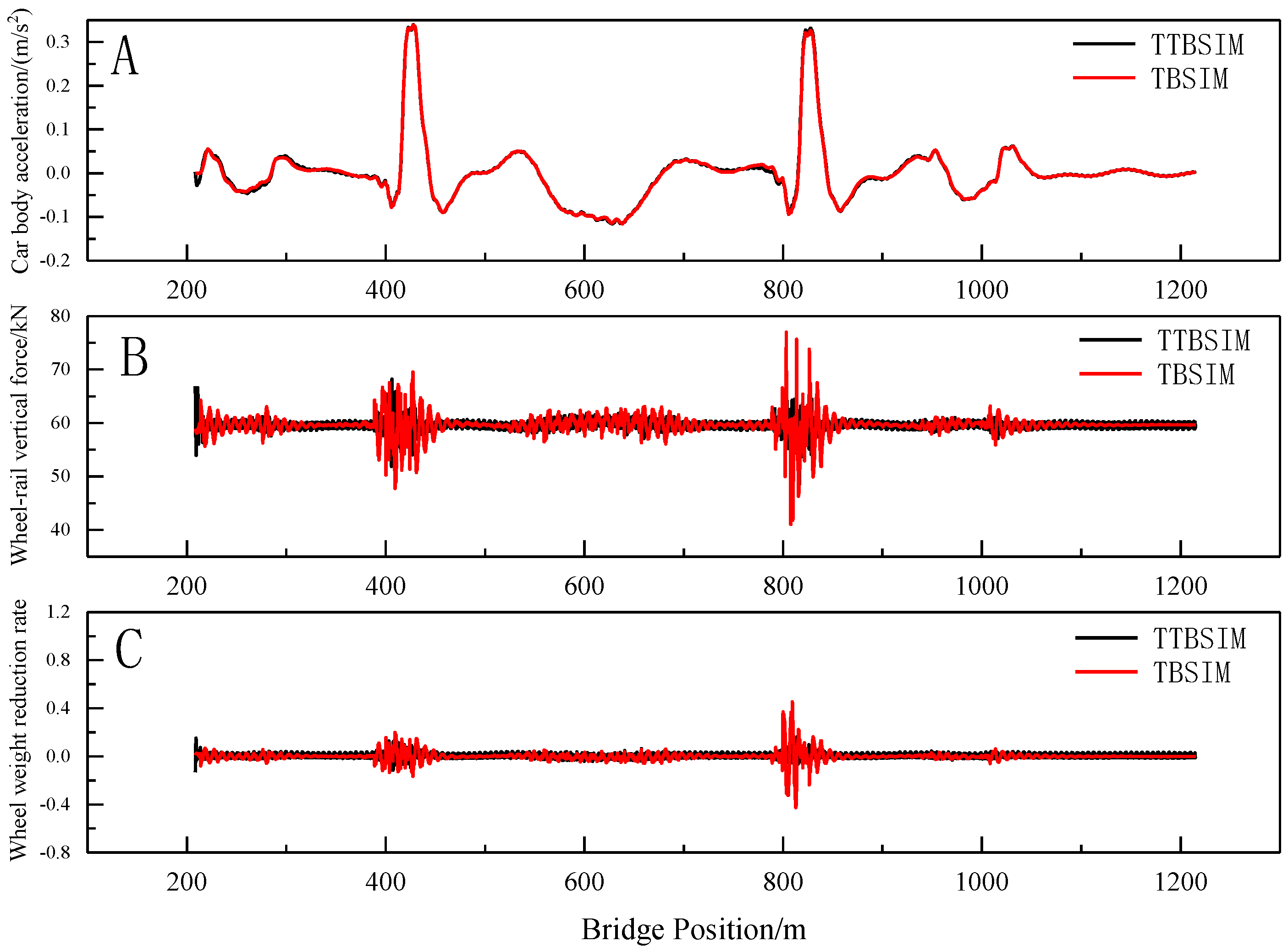
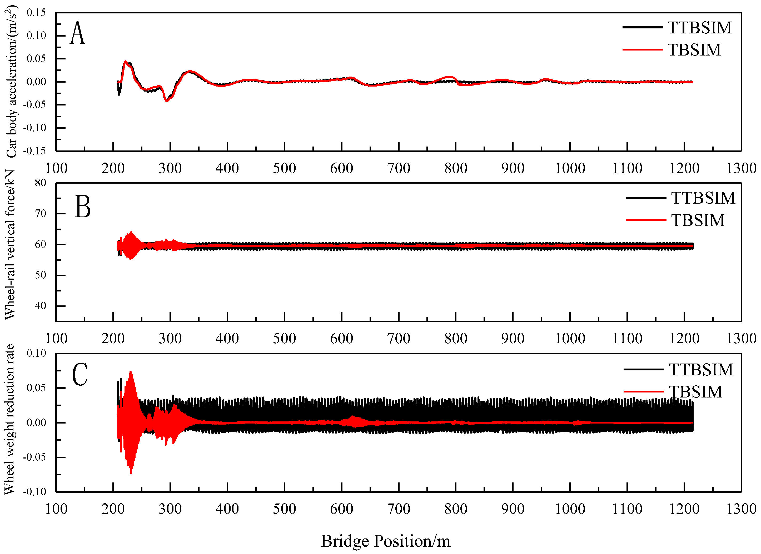
5.3. Train Vibration Response Under Different Irregularity Excitation

Under the influence of the random irregularity, the temperature-induced deformation of the cable beam, and the settlement of the auxiliary pier, the TTBSIM model and the TBSIM model are utilized to calculate the vertical acceleration of the car body, wheel–rail vertical force, and wheel-weight reduction rate during the entire process of the train entering and exiting the bridge, as illustrated in Figure 20, Figure 21 and Figure 22.

From the figure, it is evident that, when comparing the train vibration response under different excitation conditions, the distribution pattern of the car body vertical acceleration calculated by both the TTBSIM model and the TBSIM model are essentially consistent. Similarly, the distribution patterns of the wheel–rail vertical force and wheel weight reduction rate align closely. Notably, locations with sudden stiffness changes, such as the bridge tower, exhibit higher values for the wheel–rail vertical force and wheel weight reduction rate as obtained from the train–bridge dynamic coupling model.

The long-wave vertical deformation of the large-span, cable-stayed bridge significantly influences the vibration acceleration of the car body and, consequently, affects the ride comfort. To calculate the impact of this vertical deformation on the acceleration of the train body, the train–bridge dynamic coupling model is employed. In this model, the track structure is simplified as a second-phase constant load applied to the main beam. This simplification not only reduces the model complexity but also enhances the computational efficiency of the program.

6. Conclusions

(1)

For the BT, the LT, and the USBT, if the minimum wavelength of the bridge deformation exceeds 6, 10, and 16 m, respectively, the rail deformation can accurately mirror the bridge deformation. Otherwise, it becomes essential to establish a comprehensive track–bridge model to accurately capture the rail deformation.

(2)

The minimum wavelength of the long-span, cable-stayed bridge tends to decrease with an increase in the number of the auxiliary pier and a decrease in the cable-stay stiffness ratio under complex loads. While the addition of the auxiliary pier in long-span, cable-stayed bridges can effectively minimize the mid-span displacements of the bridge’s tower and the main span, it affects the smoothness of long waves in the vicinity of the bridge pier. The vertical deformation wavelength range for long-span, cable-stayed bridges with main spans ranging from 200 m to 600 m is observed to be between 21.38 m and 1270.74 m.

(3)

The deformation of the cable-stayed bridge is primarily influenced by wavelengths greater than 200 m under the influence of overall loads such as the temperature and overall settlement. However, during the ingress and egress of trains, as well as local loads like the single auxiliary pier’s settlement, there may be the vertical deformation with the wavelength of approximately 200 m near the pier, impacting the overall smoothness of the bridge’s long waves.

(4)

Based on the track–bridge mapping relationship and the wavelength’s range of the vertical deformation for the cable-stayed bridge, the comparison was made between the train’s vibration of the TBSIM model and the TTBSIM model under various excitations. The simulation results are found to be essentially consistent. The impact of the vertical deformation of the long-span, cable-stayed bridge on the train’s vibration can be accurately calculated using the train–bridge dynamic coupling model. In this model, the track is simplified and considered as the second-phase’s constant load, contributing to improved computational efficiency.