Estimation of Wind Turbine Blade Icing Volume Based on Binocular Vision

Abstract

Icing on wind turbine blades in cold and humid weather has become a detrimental factor limiting their efficient operation, and traditional methods for detecting blade icing have various limitations. Therefore, this paper proposes a non-contact ice volume estimation method based on binocular vision and improved image processing algorithms. The method employs a stereo matching algorithm that combines dynamic windows, multi-feature fusion, and reordering, integrating gradient, color, and other information to generate matching costs. It utilizes a cross-based support region for cost aggregation and generates the final disparity map through a Winner-Take-All (WTA) strategy and multi-step optimization. Subsequently, combining image processing techniques and three-dimensional reconstruction methods, the geometric shape of the ice is modeled, and its volume is estimated using numerical integration methods. Experimental results on volume estimation show that for ice blocks with regular shapes, the errors between the measured and actual volumes are 5.28%, 8.35%, and 4.85%, respectively; for simulated icing on wind turbine blades, the errors are 5.06%, 6.45%, and 9.54%, respectively. The results indicate that the volume measurement errors under various conditions are all within 10%, meeting the experimental accuracy requirements for measuring the volume of ice accumulation on wind turbine blades. This method provides an accurate and efficient solution for detecting blade icing without the need to modify the blades, making it suitable for wind turbines already in operation. However, in practical applications, it may be necessary to consider the impact of illumination and environmental changes on visual measurements.

1. Introduction

Wind energy has become an essential component of the global pursuit of sustainable and renewable energy sources [1]. With the increasing deployment of wind turbines in cold and humid weather conditions, blade icing has become a focal point of concern [2]. Ice accretion on wind turbine blades can lead to decreased aerodynamic efficiency [3], reduced power output [4], increased mechanical loads [5], and safety hazards due to ice shedding [3]. These issues highlight the necessity for effective detection and management of blade icing on wind turbines.

The traditional methods for detecting and quantifying icing on wind turbine blades include data analysis, sensor-based detection, and meteorological assessments. For instance, Skrimpas et al. [6] proposed a method based on vibration and power curve analysis, which is effective in detecting large areas of icing. However, its sensitivity to localized, small-scale, or unevenly distributed icing is relatively low. Furthermore, it is susceptible to disturbances from nacelle vibrations and wind speed variations during operation, which can affect its detection accuracy. Zhao et al. [7] demonstrated that ultrasonic imaging technology performs well in detecting thick ice layers and large blade structures. However, its sensitivity decreases for thin ice layers, and its performance is further reduced when the blade surface roughness increases, limiting its application under complex surface conditions. Wang et al. [8] adopted ultrasonic guided waves combined with Principal Component Analysis (PCA) to eliminate the influence of temperature, achieving high-precision ice monitoring. Nonetheless, the deployment costs are high, requiring multiple ultrasonic sensors installed on the blade, which are prone to environmental noise and blade vibration, thereby reducing detection stability. Roberge et al. [9] proposed a low-cost detection method based on a heated cylindrical probe, which can effectively monitor the onset and intensity of icing. However, it is sensitive to wind speed and temperature in extreme weather conditions, potentially resulting in errors. In recent years, significant progress has been made in wind turbine blade icing detection technologies driven by data-driven and intelligent methods. Xu et al. [10] employed a particle swarm optimization algorithm combined with a support vector machine to predict blade icing conditions, achieving high accuracy. However, this approach requires extensive data preprocessing, and its generalizability across different wind farms remains to be validated. Li et al. [11] proposed the 1D-CNN-SBiGRU model, which achieves high-precision predictions through feature selection and deep learning, exhibiting strong anti-interference capability. However, the computational complexity of this model may affect real-time performance. Cheng et al. [12] introduced the IcingFL model within a federated learning framework, which achieves high-accuracy icing detection and data privacy protection through local model training and global model aggregation. However, federated learning entails high communication costs. These studies indicate that wind turbine blade icing detection is transitioning from traditional methods to data-driven and intelligent optimization approaches, with future advancements needed in real-time performance, cost-effectiveness, and adaptability. Wang et al. [13] proposed a unified semi-supervised contrastive learning framework, which integrates supervised and unsupervised learning to address the challenges of scarce labeled data and class imbalance. This method demonstrates strong robustness and generalization across multiple datasets. Jiang et al. [14] proposed a method that combines a spatiotemporal attention mechanism with an adaptive weight loss function. By extracting spatiotemporal features from SCADA data and dynamically adjusting class weights, this approach effectively addresses data imbalance issues. However, the model’s training relies heavily on high computational resources. Wang et al. [15] developed a blade icing monitoring and de-icing device based on machine vision. By integrating laser sensors and ultrasonic de-icing technology, this approach achieves a balance between real-time performance and precision. Although the technology performs well on small-scale wind turbines, its adaptability to extreme environments still requires optimization.

With advances in imaging technology and computational algorithms, computer vision offers a promising alternative for non-contact detection of blade icing [16]. In particular, binocular vision technology can reconstruct three-dimensional structures from two-dimensional images taken from slightly different viewpoints. This technology has been successfully applied in various fields such as 3D reconstruction [17], robotic navigation [18], autonomous driving and environmental monitoring [19]. In the detection of blade icing on wind turbines, employing binocular vision to capture images of blade icing and combining image processing techniques to extract and analyze information is a feasible detection method. This approach can measure ice thickness without modifying the blades, making it suitable for wind turbines already in operation. Inspections can be conducted via drones or robots, further achieving unmanned operation. Moreover, the detection results are intuitive, facilitating subsequent processing by staff. This binocular vision-based scheme provides a new reliable path for blade icing detection on wind turbines.

To further enhance the detection performance of binocular vision systems, selecting an appropriate image processing algorithm is particularly important. The Census transform, known for its robustness to illumination changes, fast execution speed, and ease of implementation, has been widely used in real-time 3D measurement and other image processing tasks. However, this algorithm also has drawbacks, such as dependence on the central pixel, sensitivity to noise, and poor performance in weakly textured regions [20].

Addressing these issues, De-Maeztu et al. [21] proposed a stereo matching algorithm combining gradient similarity and adaptive support weights, improving matching accuracy by replacing the traditional intensity similarity measure. Mei et al. [22] proposed a fusion method based on Absolute Difference (AD) and Census cost, compensating for the shortcomings of single-cost approaches. By combining the AD-Census transform with improved cross-region support and utilizing a scanline optimization framework, their algorithm demonstrated excellent performance in the Middlebury benchmark tests. Lee et al. [23] introduced an efficient one-shot local disparity estimation algorithm, utilizing a trimodal cross Census transform and advanced support weights to enhance the accuracy of disparity maps, extending it to video disparity estimation. Hosni et al. [24] combined the Sum of Absolute Differences (SAD) with gradient information, using the absolute sum of the gradient values of the matching points and the absolute gray-level differences within the support window as the basis for the matching cost. Wang et al. [25] developed a real-time high-quality stereo vision system based on a Field Programmable Gate Array (FPGA), combining AD-Census cost initialization, cross-based aggregation, and semi-global optimization to achieve high-quality depth results on FPGA. The system can flexibly adjust image resolution, parallelism, and support region size for optimal efficiency. Cheng et al. [26] proposed a non-local cost aggregation algorithm for stereo matching based on a cross-tree structure, edges, and superpixel priors. By performing non-local cost aggregation through the cross-structure of horizontal and vertical trees and combining edge and superpixel priors, it effectively avoids erroneous aggregation across depth boundaries. Lee et al. [27] introduced an improved Census transform algorithm for noise-robust stereo matching, enhancing matching accuracy and robustness by symmetrically comparing pixel intensities separated by a certain distance within the matching window. Lv et al. [28] converted color images into the HSV (hue, saturation, value) space, established a hue absolute difference cost calculation function, and fused it with the Census cost. Zhou et al. [29] proposed a multi-feature fusion stereo matching algorithm based on an improved Census transform, enhancing matching accuracy and noise resistance by introducing gradient cost, edge, and feature point information during the cost computation stage. Yang et al. [30] proposed a stereo matching algorithm based on an improved Census transform, enhancing robustness to noise by introducing weighted average computation to replace the central pixel in the traditional Census transform.

Based on the aforementioned studies, this paper proposes a stereo matching algorithm that employs dynamic windows combined with multiple features and reordering. Gradient, color, and other information are fused to generate the final matching cost. The cost is aggregated using a cross-based support region method. Finally, a Winner-Take-All (WTA) method [31] and multi-step optimization are used to generate the final disparity map. Subsequently, image processing techniques combined with 3D reconstruction methods are used to model the geometric shape of the ice, and its volume is estimated. The proposed method aims to overcome the limitations of existing methods, providing a non-contact, accurate, and efficient solution for ice volume estimation.

The remainder of this paper is organized as follows: Section 2 provides a detailed description of the binocular vision-based method, including computation methods for stereo matching and volume calculation. Section 3 presents the results and validations of the proposed method under various experimental conditions. Finally, Section 4 discusses the significance of the research findings and proposes future research directions.

2. Principle and Method

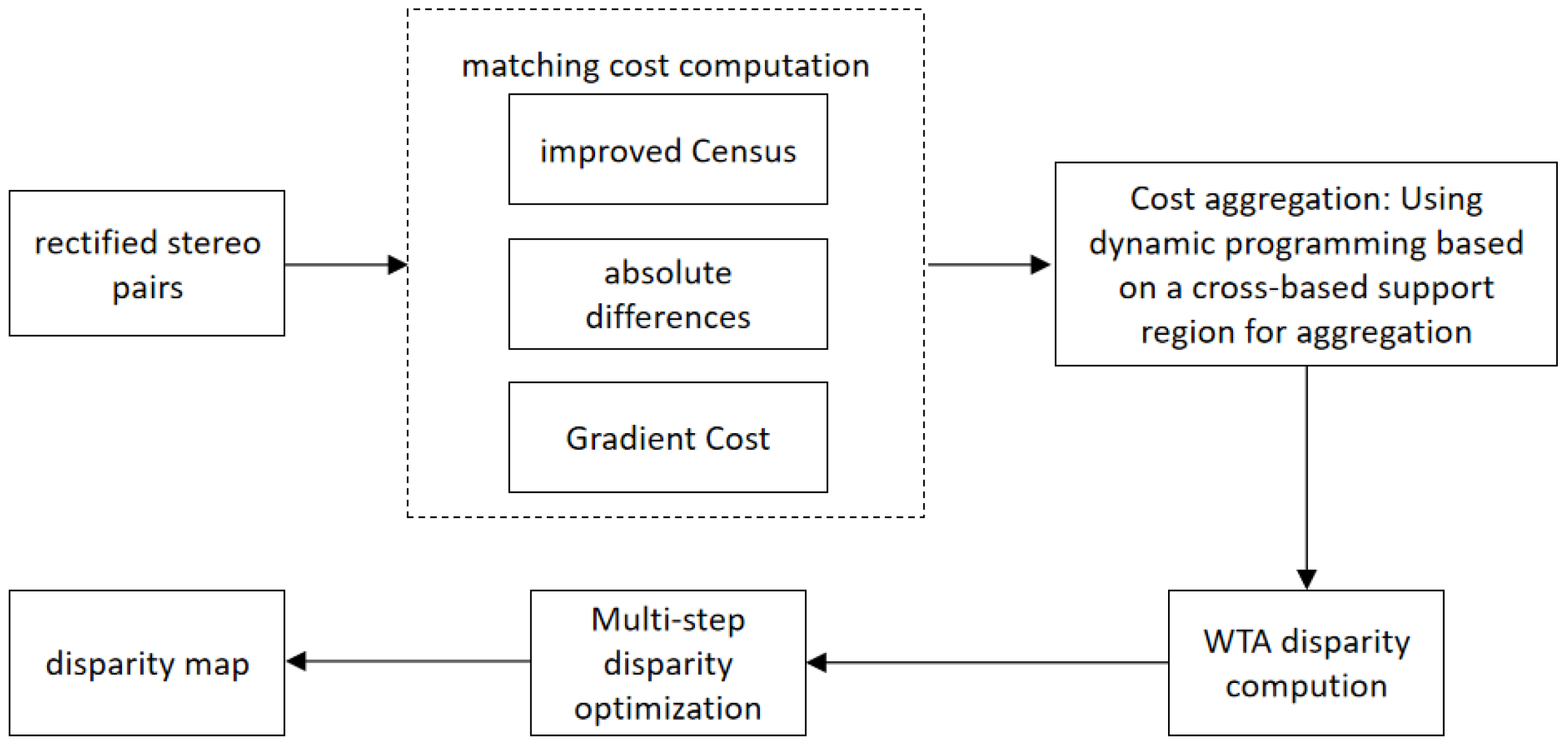
2.1. Stereo Matching

Due to the indistinct features and weak textures of ice accretion on wind turbine blades, traditional Census transform algorithms that rely on the central pixel of the window are susceptible to noise interference in weakly textured and complex textured regions, leading to reduced matching accuracy. To address these issues, this paper proposes an improved stereo matching algorithm.

The proposed algorithm primarily consists of four steps: cost computation, cost aggregation, disparity computation, and disparity optimization. Figure 1 illustrates the flowchart of the proposed algorithm. The specific steps are as follows:

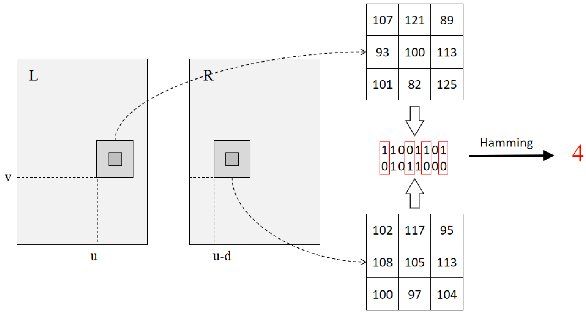
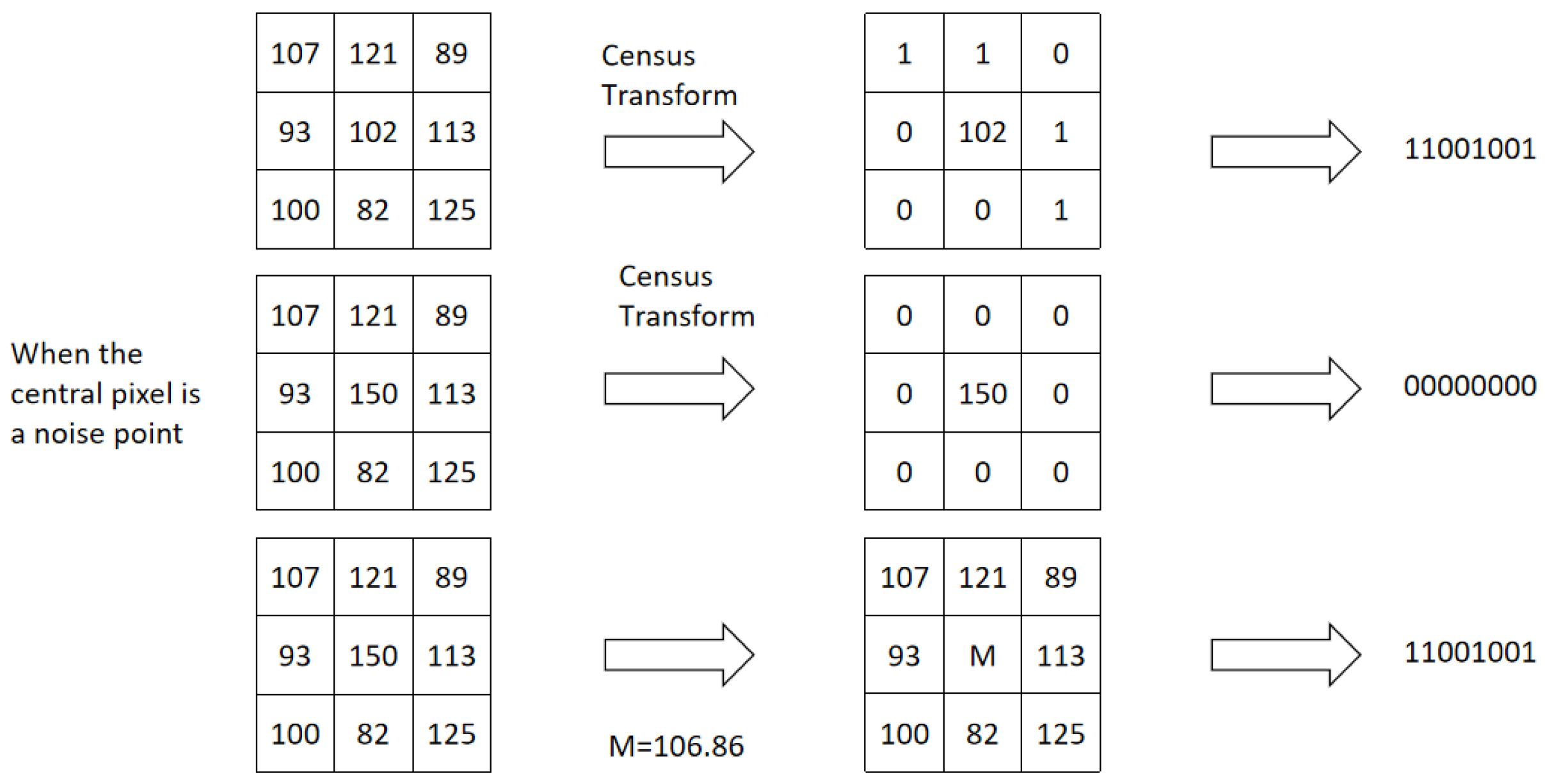
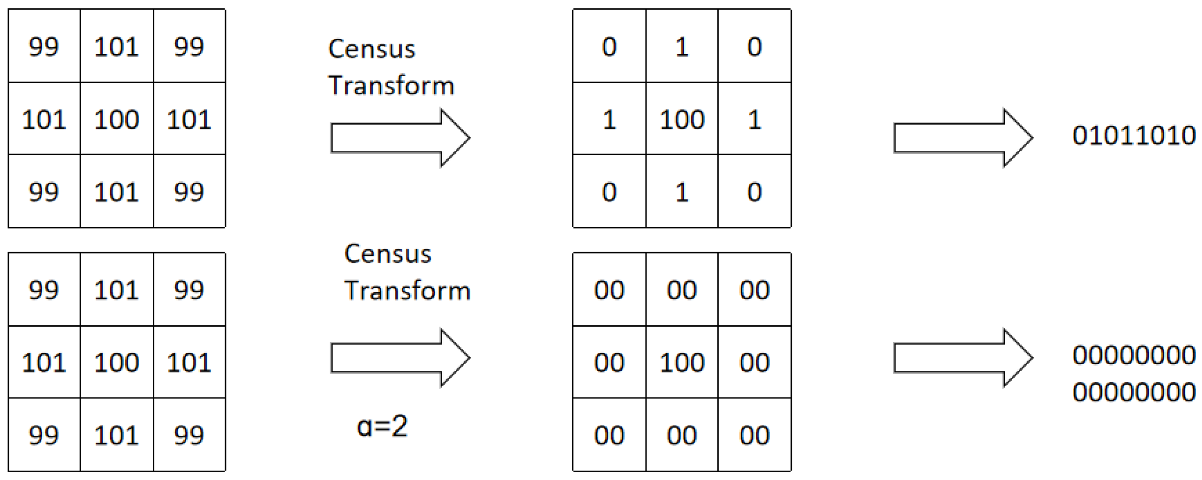
• Initial Cost Computation: The initial matching cost is obtained by combining an improved Census transform with gradient and color information.
• Cross-Based Cost Aggregation: We adopt the adaptive window method based on cross-based regions from reference [24] and introduce a unidirectional dynamic programming cost aggregation algorithm for cost aggregation.
• Disparity Computation: The initial disparity map is computed using the Winner-Take-All (WTA) method.
• Disparity Optimization: Multiple methods are employed to optimize the initial disparity map.

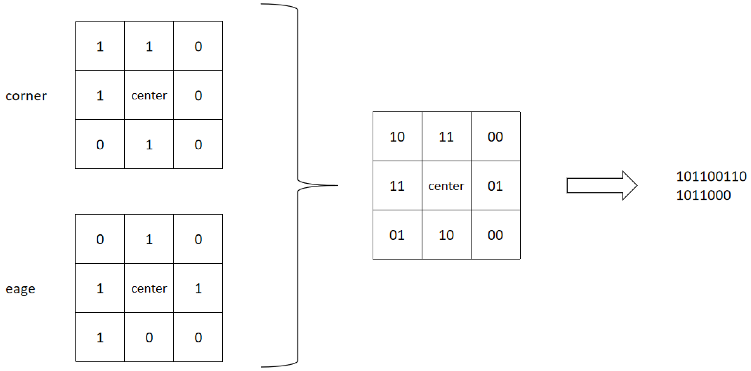
2.1.1. Matching Cost Calculation

The basic principle of the traditional Census transform involves traversing the image with a rectangular window, typically selecting the gray value of the central pixel as the reference. The gray values of all pixels within the window are compared with this reference value, and the size relationships are represented by 0 or 1. Essentially, the Census transform encodes the gray values of an image into a binary bit stream, indicating the relative size relationships of neighboring pixels to the central pixel. The transformation process can be expressed as

$$I_{\mathrm{census}}\left(p\right)=\underset{q\in N_p}{⨂}\xi [I\left(p\right),I\left(q\right)]$$

(1)

where $I_{\mathrm{census}}\left(p\right)$ represents the Census transform code of pixel p; p is the central pixel; q is a pixel within the neighborhood window; ⨂ denotes the bitwise concatenation operator; $I\left(p\right)$ is the intensity value of the central pixel; $I\left(q\right)$ is the intensity value of the neighboring pixel; and $N_p$ is the set of pixels in the neighborhood window centered at p. The function $\xi \left[I\right(p),I(q\left)\right]$ is defined as:

$$\xi [I\left(p\right),I\left(q\right)]=\left\{\begin{array}{cc}0,\hfill & I\left(q\right)\le I\left(p\right)\hfill \\ 1,\hfill & I\left(q\right)>I\left(p\right)\hfill \end{array}\right.$$

(2)

After these calculations, the Census transform codes of each pixel in the left and right images are obtained. Then, by computing the Hamming distance, the matching cost is derived. For any disparity value d within the disparity search range, the Hamming distance between the Census transform code of pixel p in the left image and the corresponding pixel $(p-d)$ in the right image is calculated as follows:

$$C_{\mathrm{cen}}(p,d)=\mathrm{Hamming}\left(C_{\mathrm{cen},\mathrm{L}}\left(p\right),C_{\mathrm{cen},\mathrm{R}}(p-d)\right)$$

(3)

where $C_{\mathrm{cen}}(p,d)$ represents the Census cost of pixel p at disparity d; $C_{\mathrm{cen},\mathrm{L}}\left(p\right)$ is the Census transform code of pixel p in the left image; and $C_{\mathrm{cen},\mathrm{R}}(p-d)$ is the Census transform code of pixel $(p-d)$ in the right image. The calculation process described above is illustrated in Figure 2.

The traditional Census transform heavily relies on the gray value of the central pixel and is sensitive to image noise. This sensitivity may lead to mismatches under noisy conditions, reducing matching accuracy. To mitigate mismatches caused by noise and improve the robustness of the algorithm, this paper proposes an improved Census transform for computing the matching cost.

First, the image gradient is calculated, and the window size is dynamically adjusted based on the gradient values. In high-gradient regions, smaller windows are used to accurately capture details; in low-gradient regions, larger windows are employed to suppress noise and enhance the stability of feature extraction. The window size is defined as:

$$\mathrm{windowSize}=\left\{\begin{array}{cc}7\times 7,\hfill & \mathrm{if}{G}_{i,j}>T\hfill \\ 9\times 9,\hfill & \mathrm{if}{G}_{i,j}\le T\hfill \end{array}\right.$$

(4)

where $G_{i,j}$ is the gradient magnitude at pixel $(i,j)$, and T is a predefined gradient threshold.

Next, the gray values within the window are sorted, the maximum and minimum values are removed, and the mean of the remaining values is calculated. This mean is used as the new central pixel value and reference value, against which the gray values of neighboring pixels in the window are compared. Figure 3 illustrates the limitations of the traditional Census transform and compares it with the proposed improved Census transform. It can be observed that even when the central pixel is disturbed, the improved bit string is less affected. Therefore, the algorithm reduces dependence on the central pixel.

To further enhance robustness, we introduce a noise tolerance parameter to the reference value and use two binary bits to represent three states, defined as:

$$\xi \left[I\left(p\right),I\left(q\right)\right]=\left\{\begin{array}{cc}10,\hfill & \mathrm{if}I\left(q\right)>\overline{I\left(p\right)}+\alpha \hfill \\ 01,\hfill & \mathrm{if}I\left(q\right)<\overline{I\left(p\right)}-\alpha \hfill \\ 00,\hfill & \mathrm{otherwise}\hfill \end{array}\right.$$

(5)

where $\overline{I\left(p\right)}$ is the reference value, and $\alpha$ is the noise tolerance parameter.

As shown in Figure 4, in flat regions, the gray values of neighboring pixels are similar. The traditional Census transform yields significant fluctuations in the binary sequences obtained, whereas the improved Census transform effectively resists noise interference. Its transformation results remain consistent, demonstrating good robustness. In this experiment, the noise threshold is set to $\alpha =2$.

After the aforementioned adjustments, the dependence on the central pixel has been effectively reduced; however, the information within the image matching window is still not fully utilized. Therefore, this paper introduces edge point information and corner point information to improve the algorithm’s performance in weakly textured and repetitive textured regions.

Firstly, the input image undergoes edge detection using the Canny algorithm, and it is then encoded as:

$$E\left(q\right)=\left\{\begin{array}{cc}1,\hfill & \mathrm{if}q\mathrm{is}\mathrm{an}\mathrm{edge}\mathrm{point}\hfill \\ 0,\hfill & \mathrm{if}q\mathrm{is}\mathrm{not}\mathrm{an}\mathrm{edge}\mathrm{point}\hfill \end{array}\right.,q\in {\mathsf{\Omega }}_{\mathrm{image}}$$

(6)

Next, the Harris corner detection algorithm is used to compute the corner responses of the image, which are also encoded as:

$$C\left(q\right)=\left\{\begin{array}{cc}1,\hfill & \mathrm{if}q\mathrm{is}\mathrm{a}\mathrm{corner}\mathrm{point}\hfill \\ 0,\hfill & \mathrm{if}q\mathrm{is}\mathrm{not}\mathrm{a}\mathrm{corner}\mathrm{point}\hfill \end{array}\right.,q\in {\mathsf{\Omega }}_{\mathrm{image}}$$

(7)

Finally, the fusion encoding process of corner and edge information is illustrated in Figure 5.

By combining the improved Census transform with corner and edge information, we perform fusion encoding resulting in a four-bit binary code. Based on this, the Hamming distance is calculated to obtain the cost value.

Using the above method can effectively handle situations where the overall brightness of the two images is inconsistent. The window-based method is more robust to image noise and has certain robustness to weak textures, better reflecting the true correlation. However, its disadvantage is that it can produce ambiguity in repetitive textures. To alleviate the ambiguity problem of repetitive textures, we further form a fusion cost by using the improved Census cost, Absolute Difference (AD) cost, and gradient cost.

The Absolute Difference cost is defined as:

$$C_{\mathrm{AD}}(p,d)=\sum _{i\in \{R,G,B\}}\left|I_i^{\mathrm{Left}}\left(p\right)-I_i^{\mathrm{Right}}(p-d)\right|$$

(8)

where $C_{\mathrm{AD}}(p,d)$ represents the Absolute Difference (AD) cost of pixel p at disparity d. $I_i^{\mathrm{Left}}\left(p\right)$ is the pixel value of the i-th color channel (R, G, or B) at position p in the left image, and $I_i^{\mathrm{Right}}(p-d)$ is the pixel value of the i-th color channel at position $p-d$ in the right image. The position $p-d$ is calculated from pixel p in the left image based on disparity d.

The gradient cost is defined as:

$$C_{\mathrm{gradient}}(p,d)={\displaystyle \frac{1}{3}}\sum _{i\in \{R,G,B\}}\left|\sqrt{{\left({\nabla }_x{I}_i^{\mathrm{Left}}\left(p\right)\right)}^2+{\left({\nabla }_y{I}_i^{\mathrm{Left}}\left(p\right)\right)}^2}-\sqrt{{\left({\nabla }_x{I}_i^{\mathrm{Right}}(p-d)\right)}^2+{\left({\nabla }_y{I}_i^{\mathrm{Right}}(p-d)\right)}^2}\right|$$

(9)

where $C_{\mathrm{gradient}}(p,d)$ represents the gradient cost of pixel p at disparity d. ${\nabla }_x{I}_i^{\mathrm{Left}}\left(p\right)$ and ${\nabla }_y{I}_i^{\mathrm{Left}}\left(p\right)$ denote the gradients of the i-th color channel at position p in the left image in the x and y directions, respectively; ${\nabla }_x{I}_i^{\mathrm{Right}}(p-d)$ and ${\nabla }_y{I}_i^{\mathrm{Right}}(p-d)$ denote the gradients of the i-th color channel at position $p-d$ in the right image in the x and y directions, respectively.

The combined normalized cost is defined as:

$$C(p,d)=\left(1-exp\left(-{\displaystyle \frac{C_{\mathrm{cen}}(p,d)}{{\lambda }_{\mathrm{cen}}}}\right)\right)+\left(1-exp\left(-{\displaystyle \frac{C_{\mathrm{AD}}(p,d)}{{\lambda }_{\mathrm{AD}}}}\right)\right)+\left(1-exp\left(-{\displaystyle \frac{C_{\mathrm{gradient}}(p,d)}{{\lambda }_{\mathrm{grad}}}}\right)\right)$$

(10)

where $C(p,d)$ represents the total cost of pixel p at disparity d. $C_{\mathrm{cen}}(p,d)$ denotes the Census transform cost of pixel p at disparity d. $C_{\mathrm{AD}}(p,d)$ denotes the Absolute Difference cost of pixel p at disparity d. $C_{\mathrm{gradient}}(p,d)$ denotes the gradient cost of pixel p at disparity d. ${\lambda }_{\mathrm{cen}}$, ${\lambda }_{\mathrm{AD}}$, and ${\lambda }_{\mathrm{grad}}$ are parameters for the Census transform cost, Absolute Difference cost, and gradient cost, respectively.

2.1.2. Cross-Based Cost Aggregation

Cost aggregation plays a crucial role in stereo matching and image processing by smoothing matching costs, reducing the influence of noise, and enhancing the stability and robustness of the matching process. It is particularly important in scenarios involving illumination changes, occlusions, and viewpoint differences. Cost aggregation can smooth disparity maps, reduce jagged effects and discontinuities, and improve matching performance in low-texture regions, thereby achieving higher-quality disparity estimations. In this paper, we adopt the improved cross-based region method from reference [24] for cost aggregation, where the construction rules for the cross arms are defined as:

• $D_c(p_1,p)<{\tau }_1$ and $D_c(p_1,p_1+(1,0))<{\tau }_1$;
• $D_s(p_1,p)<L_1$;
• $D_c(p_1,p)<{\tau }_2$, when $L_2<D_s(p_1,p)<L_1$.

Rule 1 ensures that the color difference between pixels $p_1$ and p is less than the threshold ${\tau }_1$, while also limiting the color difference between $p_1$ and its forward pixel $p_1+(1,0)$ to be less than ${\tau }_1$. This prevents the cross arm from crossing edge pixels.

Rules 2 and 3 provide more flexible control by introducing a larger threshold $L_1$, allowing more pixels to be included in weakly textured regions. When the color difference exceeds a smaller threshold $L_2$ ($L_2<L_1$), the cross arm only extends to points with significantly smaller color differences, ensuring it does not extend beyond $L_1$.

After successfully constructing the cross arms, the support region of pixel p is formed by merging the horizontal arms of all pixels on its vertical arm, as shown in Figure 6.

Once the support region of pixel p has been constructed, a two-pass cost aggregation can be performed:

Pass 1: For all pixels, sum the cost values of the pixels on their horizontal arms and store them as temporary values.

Pass 2: For all pixels, sum the temporary values stored in the first step for the pixels on their vertical arms to obtain the final aggregated cost value for that pixel. To keep the aggregated value within a small and controllable range, the final aggregated cost value needs to be divided by the total number of pixels in the support region, as illustrated in Figure 7.

To further enhance the accuracy of cost aggregation and reduce matching errors, a unidirectional dynamic programming cost aggregation algorithm is introduced. This algorithm optimizes along eight directions: left, right, up, down, upper right, lower right, upper left.

The path cost for pixel p along a certain path r is defined as:

$$L_r(p,d)=C(p,d)+min\left\{\begin{array}{c}{L}_r(p-r,d)\hfill \\ L_r(p-r,d-1)+P_1\hfill \\ L_r(p-r,d+1)+P_1\hfill \\ \underset{t}{min}{L}_r(p-r,t)+P_2\hfill \end{array}\right\}-\underset{t}{min}{L}_r(p-r,t)$$

(11)

This formula calculates the aggregated cost of pixel p at disparity d, incorporating penalty terms $P_1$ and $P_2$ for disparity changes. Here, $P_1$ penalizes small disparity variations, while $P_2$ controls larger disparity jumps. The subtraction of $\underset{t}{min}{L}_r(p-r,t)$ normalizes the current cost relative to the minimum cost of the previous pixel along the path, preventing instability due to excessively large values.

The specific rules for setting $P_1$ and $P_2$ are as follows:

• $P_1={\mathsf{\Pi }}_1$, $P_2={\mathsf{\Pi }}_2$, if $D_1<{\tau }_{S0}$ and $D_2<{\tau }_{S0}$;
• $P_1={\mathsf{\Pi }}_1/4$, $P_2={\mathsf{\Pi }}_2/4$, if $D_1<{\tau }_{S0}$ and $D_2>{\tau }_{S0}$;
• $P_1={\mathsf{\Pi }}_1/4$, $P_2={\mathsf{\Pi }}_2/4$, if $D_1>{\tau }_{S0}$ and $D_2<{\tau }_{S0}$;
• $P_1={\mathsf{\Pi }}_1/10$, $P_2={\mathsf{\Pi }}_2/10$, if $D_1>{\tau }_{S0}$ and $D_2>{\tau }_{S0}$.

In these equations, $D_1$ represents the color difference between pixel p and its preceding pixel $p-r$, and $D_2$ represents the color difference between pixel $p-r$ and its preceding pixel $p-2r$. The parameters ${\mathsf{\Pi }}_1$ and ${\mathsf{\Pi }}_2$ are preset fixed penalty values, typically determined empirically or through experiments. ${\tau }_{S0}$ is a predefined color difference threshold used to assess the color similarity between pixels.

Finally, the optimized cost values $L_r(p,d)$ from the eight directions are averaged to obtain the aggregated cost value for pixel p:

$$C_2(p,d)={\displaystyle \frac{1}{8}}\sum _r{L}_r(p,d)$$

(12)

where $C_2(p,d)$ represents the aggregated cost value of pixel p at disparity d.

2.1.3. Disparity Computation and Disparity Optimization

In the disparity computation, the Winner-Takes-All (WTA) method is employed to select the disparity value with the lowest cost as the optimal disparity, thereby generating the initial disparity map. However, due to differences in camera viewpoints, there may be invalid occlusion regions in the image pair where disparities cannot be reliably computed. Therefore, the initial disparity map requires multi-step optimization, including consistency checking, iterative support region voting, appropriate interpolation, and sub-pixel refinement.

For each point in the initial disparity map, the left–right consistency is checked using the following formula:

$$|D_L\left(p\right)-D_R(p-D_L\left(p\right))|\le \delta$$

(13)

where $D_L\left(p\right)$ is the disparity value at pixel p in the left disparity map, $D_R(p-D_L\left(p\right))$ is the disparity value at the corresponding pixel $p-D_L\left(p\right)$ in the right disparity map, and $\delta$ is the error tolerance, typically set to $\delta =1$. Points that pass this check are marked as valid, while those that fail are labeled as outliers.

An iterative support region voting process is then applied to the outliers. The conditions for updating an outlier’s disparity value are:

$$\left\{\begin{array}{c}\left|R\left(p\right)\right|>{\tau }_n\hfill \\ {\displaystyle \frac{n_{d_R\left(p\right)}}{\left|R\right(p\left)\right|}}>{\tau }_r\hfill \end{array}\right.$$

(14)

where $\left|R\right(p\left)\right|$ is the total number of pixels in the support region $R\left(p\right)$ around pixel p; $n_{d_R\left(p\right)}$ is the number of pixels within $R\left(p\right)$ that share the most frequently occurring disparity value, i.e., the number of votes for the mode disparity value; ${\tau }_n$ and ${\tau }_r$ are predefined thresholds.

When the support region of an outlier satisfies the above conditions, the value $d_R\left(p\right)$ is used to replace the outlier’s disparity, and it is marked as valid. This process is iteratively repeated to handle additional outliers.

Appropriate interpolation is utilized to address the remaining outliers. First, outliers are classified into occluded points and mismatched points. For occluded points, the nearest valid disparities in the left or right direction are used for replacement. For mismatched points, the nearest valid disparities in both the left and right directions are found, and the mismatched point is replaced with the smaller of the two disparity values.

Finally, sub-pixel refinement is applied to the disparity map to obtain the final disparity map.

2.2. Volume Calculation

To accurately assess the volume of the object, we employed a systematic approach that encompasses outlier detection and removal, interpolation to construct a 3D surface, and the final volume calculation.

Firstly, to enhance data quality and analytical accuracy, we utilized an outlier detection method based on k-Nearest Neighbors (k-NN). For each data point $(x_i,y_i)$, it is necessary to determine its nearest neighbors in the plane. For the i-th point, we find its k nearest neighbors (excluding itself) in the plane, denoted as:

$$\mathrm{Neighbors}\left(i\right)=\{j\mid j\in \mathrm{KNN}(i\left)\right\}$$

(15)

where $\mathrm{KNN}\left(i\right)$ represents the indices of the k nearest neighbors of the i-th point. $\mathrm{Neighbors}\left(i\right)$ is the set of neighbor point indices for the i-th point. Let $z_j^{\prime }$ be the height value of neighbor point j. To determine whether the current point is an outlier, we set a threshold $\theta =2$. If the following condition is satisfied, the point is considered an outlier and is removed:

$$|z_i^{\prime }-{\overline{z}}_{\mathrm{neighbors}}|>\theta ·{\sigma }_{\mathrm{neighbors}}$$

(16)

After data preprocessing, the next step is to construct the 3D surface. For this purpose, we applied a linear two-dimensional interpolation method to map the discrete point cloud data onto a regular grid.

Firstly, we set $N_x$ equally spaced nodes in the x-direction and $N_y$ equally spaced nodes in the y-direction. The process of generating grid nodes includes determining the grid range, calculating step sizes, and generating grid nodes. Based on the x and y coordinate ranges of the point cloud data, we determine the minimum and maximum values of the interpolation grid and then calculate the step sizes $\Delta x$ and $\Delta y$ in the x and y directions:

$$\Delta x={\displaystyle \frac{x_{max}-x_{min}}{N_x-1}}$$

(17)

$$\Delta y={\displaystyle \frac{y_{max}-y_{min}}{N_y-1}}$$

(18)

Equally spaced nodes are then generated in the x and y directions:

$$x_{\mathrm{grid}}=\{x_{min},x_{min}+\Delta x,\cdots ,x_{max}\}$$

(19)

$$y_{\mathrm{grid}}=\{y_{min},y_{min}+\Delta y,\cdots ,y_{max}\}$$

(20)

Using the generated regular grid, we compute the height values Z at each node through linear interpolation. This process smoothly maps the discrete point cloud data onto the regular grid, constructing a continuous 3D surface model.

After obtaining the 3D surface model, the next step is to calculate the object’s volume. To improve the accuracy of the volume calculation, we employed numerical integration methods. By performing double integration over the region beneath the surface, we can capture subtle variations in the surface more accurately. The calculation formula is as follows:

$$V=\underset{\mathsf{\Omega }}{\int \int }Z(x,y)dxdy$$

(21)

where $\mathsf{\Omega }$ is the projection area of the surface, and $Z(x,y)$ is the height value of the interpolated surface at coordinate $(x,y)$. There are two specific implementation methods:

1.

Sum of Heights and Unit Area Method

First, calculate the area of each grid cell S:

$$S=\Delta x\times \Delta y$$

(22)

Then, sum the height values $Z_{i,j}$ of all grid points to obtain the total height H:

$$H=\sum _{i=1}^{N_x}\sum _{j=1}^{N_y}{Z}_{i,j}$$

(23)

Finally, the volume V is calculated as:

$$V=H\times S$$

(24)

This method is simple to compute but may lead to larger errors when the grid density is low or the surface varies significantly.

2.

Trapezoidal Integration Method

Using the trapz function for more accurate numerical integration. The calculation formula is:

$$V=\mathrm{trapz}(y_{\mathrm{grid}},\mathrm{trapz}(x_{\mathrm{grid}},Z,2))$$

(25)

First, perform trapezoidal integration in the x-direction for each row to obtain the integration results of each row; then, perform trapezoidal integration in the y-direction on these results to obtain the total volume V. The trapezoidal integration method can capture the variations in the surface in all directions more accurately, significantly improving the precision of volume estimation.

In this study, we adopted both volume calculation methods: the Sum of Heights and Unit Area Method and the Trapezoidal Integration Method. Through comparison, we found that the Sum of Heights and Unit Area Method is computationally simple and suitable for cases with high grid density and smooth surface variations. However, it has larger errors when the surface varies greatly or the grid density is low. The Trapezoidal Integration Method has higher computational complexity but can capture subtle variations in the surface more precisely, making it suitable for scenarios requiring high-precision volume estimation. Considering computational efficiency and accuracy, we prioritized the Trapezoidal Integration Method for volume calculation in this paper to enhance the accuracy of the results.

3. Experimental Design and Results Analysis

3.1. Noise Resistance Experiment

To evaluate the performance and robustness of the proposed algorithm, experiments were conducted using stereo image pairs from the Middlebury dataset [32], as shown in Figure 8. One of the key evaluation metrics is the mismatch rate, which is defined as:

$$P_{\mathrm{PBM}}={\displaystyle \frac{1}{N}}\sum _{(x,y)}\left[\left|d_e(x,y)-d_r(x,y)\right|>{\sigma }_d\right],$$

(26)

where N denotes the total number of effective pixels in the evaluated image region. Here, $d_e(x,y)$ represents the disparity values estimated by the algorithm, and $d_r(x,y)$ refers to the ground truth disparity provided by the dataset. The parameter ${\sigma }_d$ is the disparity threshold. This evaluation approach ensures a fair and consistent comparison of the algorithm’s accuracy by focusing on disparity deviations beyond the acceptable range.

The implementation of the algorithm was carried out using C++ on the Visual Studio 2022 development platform. Image operations, such as reading, displaying, and saving, were performed using the OpenCV open-source vision library. The experimental hardware environment consisted of an AMD Ryzen 7 3750H processor and 16 GB of RAM.

To evaluate the noise resistance of the algorithm, salt-and-pepper noise and Gaussian noise were added to the standard test images. For salt-and-pepper noise, the coverage rates were set to 3%, 6%, 9%, and 12%. For Gaussian noise, the standard deviations were set to 2, 4, 6, and 8. The disparity maps generated from the noisy images were then used to calculate the mismatch rate in the non-occluded regions. These results were compared with those obtained using the AD-Census algorithm [24] and the SGM algorithm [33]. The final experimental results are summarized in

Table 1. Mismatch rates of different algorithms after adding salt-and-pepper noise (%).

Algorithm	0	3	6	9	12
SGM	4.99	5.72	7.32	8.16	9.87
AD-Census	4.57	5.28	5.88	6.92	8.76
Proposed algorithm	3.97	3.99	4.21	4.83	6.52

,

Table 2. Mismatch rates of different algorithms after adding Gaussian noise ($\sigma$).

Algorithm	0	2	4	6	8
SGM	4.99	8.78	11.18	14.09	16.57
AD-Census	4.57	6.20	8.30	10.15	12.21
Proposed algorithm	3.97	5.20	7.21	8.97	10.19

and

Table 3. Average running time of different algorithms (s).

Algorithm	SGM	AD-Census	Proposed Algorithm
Time	6.786	3.074	3.201

.

Based on Table 1, Table 2 and Table 3, when no noise is introduced, the average mismatching rate of the improved algorithm proposed in this paper is significantly lower compared to other algorithms. As the noise density increases, the mismatching rates of all algorithms also rise. Notably, the SGM algorithm exhibits the largest increase, indicating its highest sensitivity to noise addition, whereas the improved algorithm in this study shows the smallest increase, which is markedly lower than that of the other comparison algorithms, demonstrating strong noise resistance. Additionally, the proposed algorithm achieves competitive runtime performance with an average running time of 3.201 s, which is close to the AD-Census algorithm and much faster than the SGM algorithm, achieving a good balance between accuracy and efficiency.

3.2. Volume Estimation Experiment of Regular-Shaped Ice Blocks

The experiment utilized the HBVCAM-4M2214HD-2 V11 model binocular stereo vision camera (Huiber Vision Technology Co., Ltd., Shenzhen, China), with its detailed specifications provided in

Table 4. Parameters of the stereo camera.

Specification	Parameter
Maximum Resolution	2688 × 1520
Sensor Model	OV4689 (1/$3^{″}$)
Supply Voltage	DC 5V ± 5%
Operating Temperature Range	−30 °C to 70 °C
Field of View (FOV)	80°

. This camera satisfies general depth perception requirements and is suitable for target detection and depth measurement. The camera was mounted on an adjustable-height tripod and positioned at a distance of 0.8–0.9 m from the experimental sample to ensure optimal depth measurement accuracy. The camera angle was adjusted to be nearly perpendicular to the surface of the sample to optimize imaging quality. The spatial layout of the experimental setup and the data acquisition system is shown in Figure 9.

To verify the feasibility and accuracy of stereo vision technology in measuring the volume of ice accretion on wind turbine blades, this paper first conducted volume measurement experiments using ice blocks of regular shapes to evaluate the precision of the measurement method. Subsequently, experiments were carried out to measure the volume of ice accretion on the blades.

In the preliminary experiments, three ice blocks with different volumes and regular shapes were selected. Their volumes were measured using stereo vision technology, and the measurement errors were calculated. The experimental results are shown in Figure 10.

As shown in

Table 5. Volume measurement results and errors.

No	Volume (mm3)	Measured Volume (mm3)	Error
1	574,456.52	544,133.70	5.28%
2	427,173.91	391,503.49	8.35%
3	417,391.30	397,165.91	4.85%

, the volume measurements of ice blocks with regular shapes verified the feasibility and accuracy of the experimental method. The measurement errors for the three ice blocks with different volumes ranged from 4.85% to 8.35%. The errors mainly originated from volume loss due to ice melting during the experiment, limitations in the precision of measurement tools, and human errors during experimental operations. Larger ice blocks exhibited relatively smaller errors, while smaller ice blocks had higher measurement errors due to a higher surface area to volume ratio, leading to more significant melting losses. Overall, the experimental method demonstrated high accuracy within a certain range, but the error was more pronounced when dealing with small-volume ice blocks. To improve precision, increasing the number of repeated measurements can provide fundamental support for subsequent volume measurements of irregularly shaped objects.

3.3. Simulation Experiment of Wind Turbine Blade Ice Accretion Volume Estimation

To verify the feasibility and accuracy of stereo vision technology in measuring the volume of ice accretion on wind turbine blades, a simulated icing experiment was designed and conducted, which mainly included two parts: ice mass measurement and stereo vision image acquisition and processing.

Firstly, a specific model of a wind turbine blade made of composite material with a smooth surface was selected. The blade had a length of 0.820 m, a maximum chord length of 0.120 m, and a minimum chord length of 0.032 m. Before the experiment, the blade was carefully cleaned and dried to ensure its surface was free of any residues. An electronic balance with a precision of 0.1 g was used to measure and record the initial mass of the blade, $m_{\mathrm{before} \mathrm{ice}}$.

The icing experiment was carried out in a refrigerator, with the temperature set to $-{15}^{ \circ }\mathrm{C}$. The prepared blade model was placed in a fixed position inside the refrigerator to ensure uniform icing conditions. The blade was immersed in water, with the amount of water carefully controlled to cover the entire blade surface without causing runoff. The environmental parameters were maintained for more than 4 h, allowing the water to freeze and form a sufficiently thick ice layer on the blade surface.

After the icing process, the blade was quickly removed to prevent the ice layer from melting due to an increase in environmental temperature. The total mass of the blade after icing, $m_{\mathrm{after} \mathrm{ice}}$, was measured again using the electronic balance. The mass of the ice layer was calculated from the difference between the two measurements:

$$m_{\mathrm{ice}}=m_{\mathrm{after} \mathrm{ice}}-m_{\mathrm{before} \mathrm{ice}}$$

(27)

Based on the density of ice ${\rho }_{\mathrm{ice}}=0.92{\mathrm{g}/\mathrm{cm}}^3$, the volume of the ice layer $V_{\mathrm{ice} (\mathrm{mass} \mathrm{method})}$ was calculated:

$$V_{\mathrm{ice} (\mathrm{mass}\mathrm{method})}={\displaystyle \frac{m_{\mathrm{ice}}}{{\rho }_{\mathrm{ice}}}}$$

(28)

At the same time, the blade was photographed before and after icing using a stereo camera. The volume of the ice layer was then calculated, obtaining $V_{\mathrm{ice}(\mathrm{vision}\mathrm{method})}$.

Finally, the volumes of the ice layer obtained by the two methods were compared and analyzed. The relative error of the stereo vision measurement result with respect to the mass method was calculated:

$$\delta =\left|{\displaystyle \frac{V_{\mathrm{ice}(\mathrm{vision}\mathrm{method})}-V_{\mathrm{ice}(\mathrm{mass}\mathrm{method})}}{V_{\mathrm{ice}(\mathrm{mass}\mathrm{method})}}}\right|\times 100\%$$

(29)

The experimental results are shown in Figure 11.

This paper conducted theoretical calculations and actual measurements of the volumes of three samples, and the results are shown in

Table 6. Volume measurement results and errors.

No	Volume (mm3)	Measured Volume (mm3)	Error (%)
1	97,608.69	92,667.37	5.06%
2	197,717.39	184,961.32	6.45%
3	257,391.30	232,847.36	9.54%

. For Sample 1, the theoretical volume was 97,608.69 mm³, and the measured volume was 92,667.37 mm³, with an error of 5.06%. Sample 2 had a theoretical volume of 197,717.39 mm³ and a measured volume of 184,961.32 mm³, with an error of 6.45%. Sample 3’s theoretical volume was 257,391.30 mm³, and the measured volume was 232,847.36 mm³, with an error of 9.54%. The results show that the errors between the measured volumes and the theoretical volumes are all within 10%, indicating that the measurement method has good accuracy and reliability.

Multiple experimental results indicate that the ice accretion volumes measured by stereo vision are highly consistent with the results calculated by the mass method. The relative errors are within an acceptable range, verifying the feasibility of this technology. By estimating the ice accretion volume, the impact of ice accretion on blade mass and aerodynamic performance can be further evaluated.

4. Conclusions

This study proposed a novel method for estimating the ice accretion volume on wind turbine blades using stereo vision and improved image processing algorithms. Experimental results demonstrated that the method achieves measurement errors within 10% for both regular-shaped ice blocks and simulated blade icing, meeting practical requirements for blade ice detection and management. The proposed method offers the advantages of non-contact measurement, strong environmental adaptability, and ease of deployment, making it suitable for use on operating wind turbines without requiring physical modifications. These results establish a solid foundation for advancing wind turbine blade ice detection technology and improving operational efficiency and safety in cold climate regions.

5. Discussion

Despite these promising results, several challenges remain. The accuracy of the proposed method in handling complex ice geometries requires further improvement, particularly under extreme weather conditions. Environmental factors such as fog, high humidity, temperature fluctuations, and the presence of dust particles can significantly degrade image quality by affecting light transmission and contrast, introducing noise into the stereo images and making it challenging for the algorithm to maintain high precision. Furthermore, offshore and onshore wind farms present distinct operational challenges and algorithmic applications. Offshore wind farms often face harsher conditions, including high humidity, salt spray, and stronger winds, which can further compromise image quality and sensor performance. Additionally, the deployment and maintenance of monitoring systems in offshore environments are more complex and costly than those onshore, potentially leading to differences in the accuracy and practicality of the proposed method that require further investigation.

To address these challenges, future research should focus on optimizing the algorithm for real-time performance, enhancing robustness under varying environmental conditions. Fixed cameras installed on land could serve as a continuous monitoring tool for detecting icing and other damages, such as cracks or surface wear, while drones offer a flexible solution for inspections, especially during icing-prone seasons, though their deployment frequency and effectiveness depend on operational needs and weather conditions. Broader applications, such as monitoring ice on power lines, aircraft wings, and offshore platforms, should also be explored. Addressing these challenges will help transform the proposed method into a comprehensive and practical solution, ensuring the operational efficiency and safety of wind turbines in diverse and challenging environments.

References

1. Yasmeen, R.; Zhang, X.; Sharif, A.; Shah, W.U.H.; Dincă, M.S. The role of wind energy towards sustainable development in top-16 wind energy consumer countries: Evidence from STIRPAT model. Gondwana Res. 2023, 121, 56–71. [Google Scholar] [CrossRef]
2. Han, Y.; Lei, Z.; Dong, Y.; Wang, Q.; Li, H.; Feng, F. The Icing Characteristics of a 1.5 MW Wind Turbine Blade and Its Influence on the Blade Mechanical Properties. Coatings 2024, 14, 242. [Google Scholar] [CrossRef]
3. Zhang, T.; Lian, Y.; Xu, Z.; Li, Y. Effects of wind speed and heat flux on de-icing characteristics of wind turbine blade airfoil surface. Coatings 2024, 14, 852. [Google Scholar] [CrossRef]
4. Douvi, E.; Douvi, D. Aerodynamic characteristics of wind turbines operating under hazard environmental conditions: A review. Energies 2023, 16, 7681. [Google Scholar] [CrossRef]
5. Rekuviene, R.; Saeidiharzand, S.; Mažeika, L.; Samaitis, V.; Jankauskas, A.; Sadaghiani, A.K.; Gharib, G.; Muganlı, Z.; Koşar, A. A review on passive and active anti-icing and de-icing technologies. Appl. Therm. Eng. 2024, 250, 123474. [Google Scholar] [CrossRef]
6. Skrimpas, G.A.; Kleani, K.; Mijatovic, N.; Sweeney, C.W.; Jensen, B.B.; Holboell, J. Detection of icing on wind turbine blades by means of vibration and power curve analysis. Wind Energy 2016, 19, 1819–1832. [Google Scholar] [CrossRef]
7. Zhao, X.; Rose, J.L. Ultrasonic guided wave tomography for ice detection. Ultrasonics 2016, 67, 212–219. [Google Scholar] [CrossRef] [PubMed]
8. Wang, P.; Zhou, W.; Bao, Y.; Li, H. Ice monitoring of a full-scale wind turbine blade using ultrasonic guided waves under varying temperature conditions. Struct. Control Health Monit. 2018, 25, e2138. [Google Scholar] [CrossRef]
9. Roberge, P.; Lemay, J.; Ruel, J.; Bégin-Drolet, A. A new atmospheric icing detector based on thermally heated cylindrical probes for wind turbine applications. Cold Reg. Sci. Technol. 2018, 148, 131–141. [Google Scholar] [CrossRef]
10. Xu, J.; Tan, W.; Li, T. Predicting fan blade icing by using particle swarm optimization and support vector machine algorithm. Comput. Electr. Eng. 2020, 87, 106751. [Google Scholar] [CrossRef]
11. Li, Y.; Hou, L.; Tang, M.; Sun, Q.; Chen, J.; Song, W.; Yao, W.; Cao, L. Prediction of wind turbine blades icing based on feature Selection and 1D-CNN-SBiGRU. Multimed. Tools Appl. 2022, 81, 4365–4385. [Google Scholar] [CrossRef]
12. Cheng, X.; Shi, F.; Liu, Y.; Liu, X.; Huang, L. Wind turbine blade icing detection: A federated learning approach. Energy 2022, 254, 124441. [Google Scholar] [CrossRef]
13. Wang, Z.; Qin, B.; Sun, H.; Zhang, J.; Butala, M.D.; Demartino, C.; Peng, P.; Wang, H. An imbalanced semi-supervised wind turbine blade icing detection method based on contrastive learning. Renew. Energy 2023, 212, 251–262. [Google Scholar] [CrossRef]
14. Jiang, G.; Yue, R.; He, Q.; Xie, P.; Li, X. Imbalanced learning for wind turbine blade icing detection via spatio-temporal attention model with a self-adaptive weight loss function. Expert Syst. Appl. 2023, 229, 120428. [Google Scholar] [CrossRef]
15. Wang, F.; Niu, L.; Wang, T.; Ye, L. Wind Turbine Blade Icing Monitoring, De-Icing and Wear Prediction Device Based on Machine Vision Recognition Algorithm. In Proceedings of the 2024 IEEE 2nd International Conference on Control, Electronics and Computer Technology (ICCECT), Jilin, China, 26–28 April 2024; pp. 687–694. [Google Scholar]
16. Aminzadeh, A.; Dimitrova, M.; Meiabadi, M.S.; Sattarpanah Karganroudi, S.; Taheri, H.; Ibrahim, H.; Wen, Y. Non-Contact Inspection Methods for Wind Turbine Blade Maintenance: Techno–Economic Review of Techniques for Integration with Industry 4.0. J. Nondestruct. Eval. 2023, 42, 54. [Google Scholar] [CrossRef]
17. Wang, D.; Sun, H.; Lu, W.; Zhao, W.; Liu, Y.; Chai, P.; Han, Y. A novel binocular vision system for accurate 3-D reconstruction in large-scale scene based on improved calibration and stereo matching methods. Multimed. Tools Appl. 2022, 81, 26265–26281. [Google Scholar] [CrossRef]
18. Liu, P.; Zhang, L.; Wang, M. Measurement of Large-Sized-Pipe Diameter Based on Stereo Vision. Appl. Sci. 2022, 12, 5277. [Google Scholar] [CrossRef]
19. Zhou, S.; Zhang, G.; Yi, R.; Xie, Z. Research on vehicle adaptive real-time positioning based on binocular vision. IEEE Intell. Transp. Syst. Mag. 2021, 14, 47–59. [Google Scholar] [CrossRef]
20. Ma, J.; Jiang, X.; Fan, A.; Jiang, J.; Yan, J. Image matching from handcrafted to deep features: A survey. Int. J. Comput. Vis. 2021, 129, 23–79. [Google Scholar] [CrossRef]
21. De-Maeztu, L.; Villanueva, A.; Cabeza, R. Stereo matching using gradient similarity and locally adaptive support-weight. Pattern Recognit. Lett. 2011, 32, 1643–1651. [Google Scholar] [CrossRef]
22. Mei, X.; Sun, X.; Zhou, M.; Jiao, S.; Wang, H.; Zhang, X. On building an accurate stereo matching system on graphics hardware. In Proceedings of the 2011 IEEE International Conference on Computer Vision Workshops (ICCV Workshops), Barcelona, Spain, 6–13 November 2011; pp. 467–474. [Google Scholar]
23. Lee, Z.; Juang, J.; Nguyen, T.Q. Local disparity estimation with three-moded cross census and advanced support weight. IEEE Trans. Multimed. 2013, 15, 1855–1864. [Google Scholar] [CrossRef]
24. Hosni, A.; Bleyer, M.; Gelautz, M. Secrets of adaptive support weight techniques for local stereo matching. Comput. Vis. Image Underst. 2013, 117, 620–632. [Google Scholar] [CrossRef]
25. Wang, W.; Yan, J.; Xu, N.; Wang, Y.; Hsu, F.H. Real-time high-quality stereo vision system in FPGA. IEEE Trans. Circuits Syst. Video Technol. 2015, 25, 1696–1708. [Google Scholar] [CrossRef]
26. Cheng, F.; Zhang, H.; Sun, M.; Yuan, D. Cross-trees, edge and superpixel priors-based cost aggregation for stereo matching. Pattern Recognit. 2015, 48, 2269–2278. [Google Scholar] [CrossRef] [PubMed]
27. Lee, J.; Jun, D.; Eem, C.; Hong, H. Improved census transform for noise robust stereo matching. Opt. Eng. 2016, 55, 063107. [Google Scholar] [CrossRef]
28. Lv, C.; Li, J.; Kou, Q.; Zhuang, H.; Tang, S. Stereo matching algorithm based on HSV color space and improved census transform. Math. Probl. Eng. 2021, 2021, 1857327. [Google Scholar] [CrossRef]
29. Zhou, Z.; Pang, M. Stereo matching algorithm of multi-feature fusion based on improved census transform. Electronics 2023, 12, 4594. [Google Scholar] [CrossRef]
30. Yang, Z.; Li, Z. Stereo Matching Algorithm Based on Improved Census Transform. In Proceedings of the 2023 4th International Conference on Computer Vision, Image and Deep Learning (CVIDL), Zhuhai, China, 12–14 May 2023; pp. 422–425. [Google Scholar]
31. Chang, X.; Zhou, Z.; Wang, L.; Shi, Y.; Zhao, Q. Real-time accurate stereo matching using modified two-pass aggregation and winner-take-all guided dynamic programming. In Proceedings of the 2011 International Conference on 3D Imaging, Modeling, Processing, Visualization and Transmission, Hangzhou, China, 16–19 May 2011; pp. 73–79. [Google Scholar]
32. Scharstein, D.; Szeliski, R. High-accuracy stereo depth maps using structured light. In Proceedings of the 2003 IEEE Computer Society Conference on Computer Vision and Pattern Recognition, Madison, WI, USA, 18–20 June 2003; Volume 1. [Google Scholar]
33. Hirschmuller, H. Stereo processing by semiglobal matching and mutual information. IEEE Trans. Pattern Anal. Mach. Intell. 2007, 30, 328–341. [Google Scholar] [CrossRef] [PubMed]
Figure 1. Flowchart of the proposed algorithm.
Applsci 15 00114 g001
Figure 2. Census transformation process.
Applsci 15 00114 g002
Figure 3. Comparison of improved algorithms and traditional algorithms under the influence of noise.
Applsci 15 00114 g003
Figure 4. Comparison between the traditional Census transform and the improved Census transform.
Applsci 15 00114 g004
Figure 5. The process of fusing corner and edge information into a combined encoding.
Applsci 15 00114 g005
Figure 6. Cross construction.
Applsci 15 00114 g006
Figure 7. Cost aggregation diagram.
Applsci 15 00114 g007
Figure 8. Middlebury stereo evaluation dataset. (a) The left image of the stereo pair and the ground truth map of the Cones dataset; (b) the left image of the stereo pair and the ground truth map of the Teddy dataset.
Applsci 15 00114 g008
Figure 9. Schematic diagram of the experimental setup’s spatial layout.
Applsci 15 00114 g009
Figure 10. Experimental results. (a1a3) Photographs of the physical objects on the left; (b1b3) Disparity maps; (c1c3) Point cloud diagrams.
Applsci 15 00114 g010
Figure 11. Experimental results. (a1a3) Photographs of the physical objects on the left; (b1b3) disparity maps; (c1c3) point cloud diagrams.
Applsci 15 00114 g011