Numerical Investigation of Stratified Slope Failure Containing Rough Non-Persistent Joints Based on Distinct Element Method

Abstract

To address the critical issue of slope stability in jointed rock masses with complex and rough structural planes, a rough joint network model using the Fourier transform was proposed and applied to the Shilu open pit mine. The on-site structural plane survey results were combined with MATLAB and PFC2D to establish numerical models for slope stability analysis considering both linear-jointed and rough-jointed rock slopes. By comparing the slip body and fracture distribution, it was found that the rough-jointed slope was stabler than the linear-jointed slope. In addition, the fracture patterns and slip displacement were significantly influenced by the inclination and undulation of the bedding planes. Slip failure patterns occurred when the angle of inclination was set at 60°. The joints played a crucial role in inducing the shear strength of slope rock masses, and the slide area was mainly observed in the shallow slope surface for inclination angles of 0° and 45°, and in the middle deep area for 60° and 90°. These results demonstrated the importance of considering rough non-persistent fractures when developing a new numerical model for slope failure modes.

1. Introduction

Structural planes are commonly distributed in jointed rock masses and dominate slope failure modes. It often exhibits random network characteristics in space, resulting in apparent anisotropic mechanical properties of layered slopes [1,2,3,4]. The common features of a macro-fracture network include the dominant direction of cracks, the development of cracks, and the connectivity of cracks. Among them, the dominant direction of cracks is obvious, which reduces the shear strength and increases the likelihood of bedding sliding. The development of fractures is reflected in their length and spacing, which reduces the slope’s ability to resist external disturbances. Rain can weaken the slope by infiltrating along the cracks, increasing the likelihood of landslide instability. The connectivity results in an uneven distribution of stress concentration parts, which can ultimately lead to local or overall slope sliding. The failure and instability of slope rock masses are generally caused by the opening, closing, and expansion of internal discontinuities [5]. The modeling process of actual engineering units, considering fracture networks, is complicated, and the calculation results are easily affected by the model size. Therefore, the accuracy of modeling is required to be particularly high. At present, the mechanical analysis of complex jointed rock masses is mostly carried out at the mesoscale of the rock, and the characterization and stability analysis of the complex structure of layered slopes needs to be further investigated.

At present, as for the stability analysis of slope rock mass, many scholars have carried out systematic research through theoretical analysis and numerical simulation in remarkable depth. Li et al. [6,7] investigated the loess landslides and segmented the loess part using a two-phase framework, which successfully detected the landslide body. Feng et al. [8] aimed to optimize the design of the slope angle by dichotomy and check the stability of the slope by the finite difference numerical calculation method, and the mechanical parameters used in the simulation calculation process remain unchanged, which ensured the comparability of the calculation results. Gao et al. [9] conducted a numerical simulation analysis of the bedding rock slope model by the discrete element method and revealed its deformation and failure mechanism and stability characteristics. Considering the joint and rock mass, Zhao et al. [10] established the corresponding joint rock model based on the discrete fracture network and obtained the corresponding mechanical parameters by combining Hoek–Brown and Mohr–Coulomb criteria and obtained good slope stability analysis results in a numerical simulation. Zhang et al. [11] generated the required fracture network parameters by using field acquisition parameters and point estimation principles based on the Beacher model to reflect the randomness and uncertainty of the actual rock structure plane. Li et al. [12] analyzed and acquired an instability model of stepped sliding bedding rock landslides, based on the B-B failure criterion and M-C failure criterion. They subsequently verified the reliability of this model by using typical case of stepped sliding of jointed rock landslides in the Sandu-Libo Expressway. This research is of great relevance to stability research of slope engineering involving complex joints and holds important reference value and scientific significance. Marco Emanuele Discenza et al. [13] examined the collective strength of joints in the geological structure while studying landslides induced by geological factors. They determined the relevant values through geological surveys and subsequently developed a joint slope model. They conducted landslide stability analysis considering the geological structure. Ren et al. [14] utilized the permanent displacement history and acceleration history of the slope to assess its stability under earthquake conditions, calculating it using the Newmark method. The research shows that the surface landslide displacement process of the slope with a jointed leveling layer is mainly controlled by the slope angle. As the joint inclination angle increases, it shows more pronounced permanent displacement, which results in reduced stability. Most models that research the characterization method of the slope joint network model assume that the rock mass structural plane on the joint section is flat and linear. The current research on the stability of complex jointed slopes is mostly based on this assumption due to the limitations of related methods, which neglects the rough characteristics of the structural plane of the slope rock mass. Nasseri et al. [15] and Mustaqm et al. [16] demonstrate that the joint roughness of rock mass is genuine and significantly affects the rock mass’s mechanical properties. In order to investigate the impact of rock joint roughness on the stability of open-pit slopes, Gao et al. [17] established a relationship formula between rock shear strength and joint roughness based on indoor experiments. They further validated the correlation between joint roughness and slope shear performance through simulation studies. To further characterize the fracture network of a rock mass, Wang et al. [18] proposed a rough discrete fracture network (RDFN) model that accounts for the roughness of the joint surfaces. Fracture network models have been successively constructed based on different geometric types of RDFN models and modeling methods; these include sine curves, broken lines, and fractals. Moreover, Wang conducted the laboratory tests and numerical simulations to model the complex structural plane network of the rock mass. The results indicate significant differences in mechanical properties and failure modes between the RDFN model with different joint shapes and the straight DFN model. Rock masses with distinct joint shapes exhibit varying mechanical strength. The RDFN model and associated methodology provide a new method to model rock slopes with intricate joint network distribution while taking joint roughness into account.

This study proposes a characterization method for a rough structural plane model to investigate the stability of a bedded slope, utilizing the complex fractured rock mass of the Shilu Iron Mine. The method is based on the principle of the Fourier transform, referring to the RDFN model and modeling method. A rough discrete fracture network model is established based on in situ measurement and characterization of structural planes, reflecting the distribution characteristics of the planes. The model is optimized using the PFC code and gravity field increase method. The study exposes the failure mode characteristics for different joint fracture geometries and spatial distribution conditions. Additionally, it analyzes the influence of the joint inclination angle on the stability of the layered slope. These research results have a guiding value for engineering modeling and stability analysis of similarly complex jointed slopes.

2. Principles of the RDFN Model

Discrete fractures distributed in the natural rock mass are generally in complex shapes, as shown in Figure 1a. Scholars have conducted simulations on complex joint network models for jointed rock masses with varying geometric shapes and spatial joint distributions to analyze their mechanical problems. The discrete fractures network (DFN) model is widely used as a joint characterization model to provide research ideas and characterization models for the mechanical properties of jointed rock mass [19]. This model has been widely used to simulate the mechanical properties of fractured rock mass, like the synthetic joint mass simulation. In this work, the DFN model is used to study the influence of structure planes on the failure pattern of the slope body.

The probability statistics of the random distribution of discrete fracture networks underlie the DFN model. To simulate the model, a corresponding probability distribution function is established. Combining the joint density, joint trace length, and random seed of the simulated object can preliminarily generate the DFN model [20,21]. In the RDFN model proposed by Wang et al. [18], its accompanying characterization methods are based on these three geometric types: curve, triangular broken line, and fractal fracture network model. Nonetheless, each RDFN model has its own geometric representation function. In order to standardize the model representation method, different geometric joint models are represented via various joint trace representation models based on the Fourier transform principle. Equation (1) selects the Fourier expansion of multi-series trapezoidal waves [18].

$$f(x)=\frac{4A_{\max }}{\pi wd}{\displaystyle \sum _{n=1}^{\infty }\frac{\sin ((2n-1)wd)}{{\left(2n-1\right)}^2}}\sin ((2n-1)wx),n=1,2,3,.$$

(1)

where T (as listed in Figure 1b) refers to the period length of the waveform, A_max refers to the amplitude height, and d refers to the rising width. The rising width determines the width of the trapezoidal platform which, in turn, further determines the geometric shape of the Fourier curve. The variable ω determines the frequency of the curve, while n signifies the Fourier series of the curve.

Figure 1b displays the various geometric shapes of trapezoidal waves that correspond to Equation (1). Adjusting the aforementioned parameters enables obtaining a joint trace that conforms to the actual shape. Figure 1c shows the traditional slope model with smooth or linear joints, which neglects the roughness of the fractures. When considering the roughness of the joints, a more reliable slope model will be obtained, as shown in Figure 1d.

Table 1. Fourier parameter table of five complex curves.

No.	Amplitude (Amax)/m	Frequency (ω)	Climbing Width (d)/m	Fourier Series (n)
1	3	3	0.1	50
2	4	2	0.1	50
3	9	2	0.5	30
4	2	3	0.5	50
5	6	2	0.001	50

presents the Fourier parameters for diverse curves. Through modifying the d value of the Fourier trapezoidal wave, it is possible to establish a unified joint random discrete fracture network (RDFN) model for complex geometric shapes, such as straight lines, triangular broken lines, and rectangular steps. Using the MATLAB platform, Fourier joint models with varying trace lengths and certain densities are established based on information concerning linear discrete fracture network (DFN) joints. The primarying modeling methods are as follows: Firstly, generate Fourier curves with fixed trace lengths. Secondly, rotate them at specific angles and randomly translate them in certain areas to generate a set of linear joints. Thirdly, generate Fourier curves with different trace lengths and similarly rotate and translate them in the same area. Eventually, the RDFN joint models are generated. These joints cross each other and exhibit network characteristics.

3. The Jointed Rock Slope Models

This study focuses on the east slope of the open-pit Shilu Iron Mine in Hainan Province as the engineering research area. The predominant lithologies of the east slope are biotite granulite and enigmatized biotite granulite. Figure 2 shows the dimensions of the east slope. The rock in the footwall is granulite. The slope of this profile is 425 m high and 700 m wide, with a top width of 257.5 m and a bottom width of 157.5 m. It is 210 m high from the bottom edge of the slope and has a slope angle of 36°.

3.1. Numerical Model Based on Digital Image Processing

Images can provide information on the joint distribution of jointed rock masses. They can also be a basis for modeling jointed rock masses. The PFC2D model can be generated based on according to the digital image using the RDFN model. The procedure consisted of the following steps:

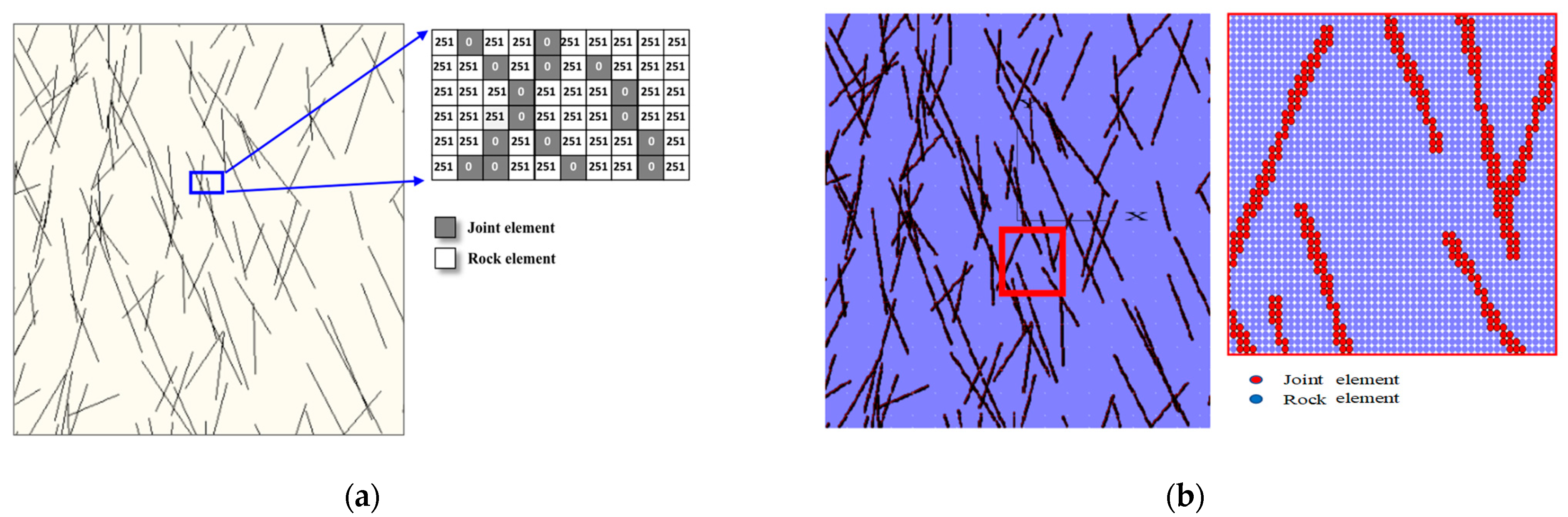
• The image was uploaded into the MATLAB 2023b program, and the RDFN gray digital image was established using the principle of gray image recognition, as illustrated in Figure 3a;
• The various types of pixel points will be classified based on gray image pixel recognition. In this case, 251 corresponds to white pixels and 0 corresponds to the black pixels. After classification, the spatial distribution coordinates of the bedrock model and joint model will be obtained.
• The joint and rock models will be grouped and assigned based on the PFC code. The mechanical modeling of the RDFN model will then ultimately be carried out, as shown in Figure 3b.

Import the RDFN and original slope models into CAD and combine them to obtain the jointed slope model. In the resulting model, the white parts represent the rock mass, the black parts represent the excavation unit, and the red parts represent the joints, as indicated in Figure 4. Rock elements and joint elements are components of the slope, while excavation elements are used to maintain the stable shape of the slope before the model iteration. The actual excavation and slope release process is simulated by deleting all excavation elements at once. Multiple sets of joint planes are generated as required, and each set of joints is composed of different joints located at a definite distance. In some actual civil engineering scenarios, the rock joints are unevenly distributed. As a result, the joint angles need to be calibrated to ensure that multiple dip joints are generated within the same model. For example, in the slope model with a joint inclination of 45°, the joint inclination follows a normal distribution that has an average of 45° and fluctuates between 30° to 60°. The resulting slope model will comprise a single set of joint dip angles, which will increase gradually from 0° to 30°, 45°, 60°, and 90°.

3.2. Mechanical Parameters

Experiments were performed in the laboratory on layered biotite granulite at varying dip angles. The physical and mechanical characteristics of biotite granulite were obtained, as presented in

Table 2. Physical and mechanical parameters of biotite granulite.

Parameters	Density/g·cm−3	Modulus of Elasticity/GPa	Uniaxial Compressive Strength/(MPa)
Value	3.527	12.0	131.73

.

The particles are bonded through contact, and the numerical simulation test for the particle flow model was conducted. The meso-parameters of the numerical models were established according to [22] and are listed in

Table 3. Micro-parameters of the particle model.

Type	Micro Parameters	Value
Intact rock	Particle radius ratio	1.66
	Density/g·cm−3	3.527
	Particle contact modulus E/GPa	14.0
	kn/ks	1.5
	Normal particle contact strength/N	100 × 106
	Shear contact strength/N	135 × 106
	Particle friction coefficient	0.86
Joint element	Joint friction coefficient, fric	0.68
	Normal contact bonding strength/N	3.00 × 106
	Shear contact bonding strength/N	4.035 × 106

.

The macroscopic parameters derived from the macroscopic parameters of biotite granulite are incorporated into the slope model to make the slope particle flow model exhibit physical and mechanical properties similar to those of realistic slopes. The stability analysis of the numerical slope model shows a failure mode that is consistent with the actual scenario.

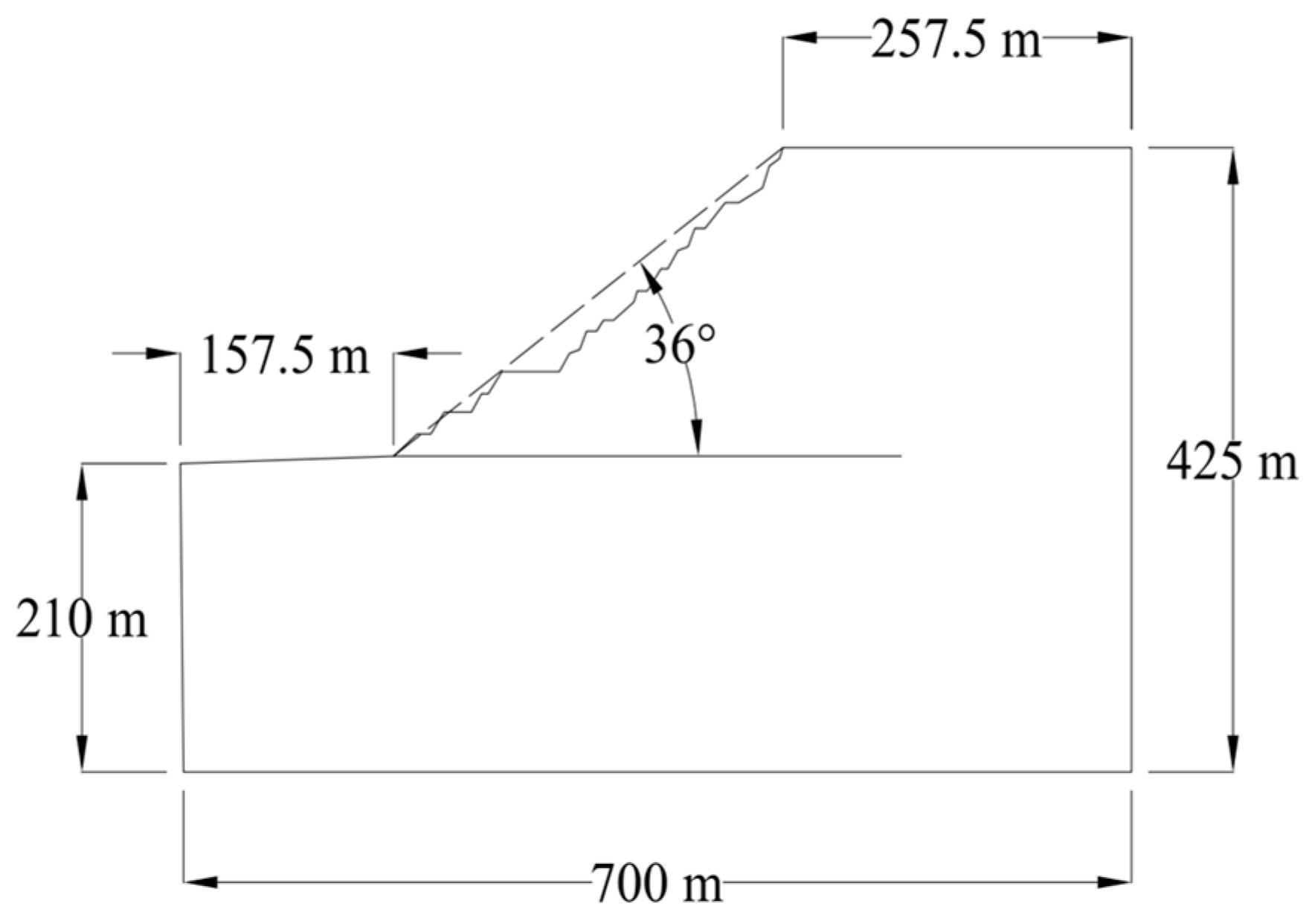
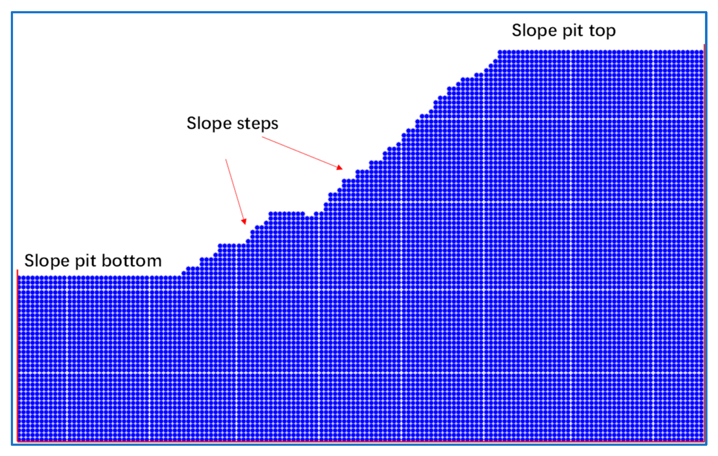
3.3. Establishment of Open-Pit Slope

The east slope is characterized by biotite granulite. The particular flow slope model of the slope profile has been established, as depicted in Figure 5. The slope model is established between 0° to 90° based on two structural plane models. The inclination angle of the structural plane will be slightly random to complete the establishment of the jointed characteristic rock slope model.

Table 4. Particle data of different PFC particle models.

Numerical Models	Dip Angle (°)	Total Number of Elements	Number of Rock Elements	Number of Joint Elements	Joint Element Proportion
Rough joint	30°	9147	7978	1169	12.7%
Linear joint	30°	9109	7924	1185	13.0%
Rough joint	60°	9703	8735	968	9.9%
Linear joint	60°	9554	8578	976	10.0%

shows some model grain data.

Perform a probability and statistics analysis based on on-site observation of the slope structural plane and mapping results. The significant parameters of the linear RDFN model are determined to be the following: an area length of 10, a joint density of 0.5, and single group inclination angles of 0°, 30°, 45°, 60°, and 90°. A digital image model of the rough RDFN slope is established and simulated in PFC2D, displayed in Figure 6i(a). Furthermore, it is transformed into derivative structural planes, with the same spectrum but varying shapes, using the Fourier transform principle in the MATLAB code. The crucial parameters of the Fourier transform are as follows: an amplitude height of 0.02 m, a frequency of 2, a Fourier series of 20, a trapezoidal wave value of 0.2, a region length of 10 m, a joint density of 0.5 traces/m, and single dip angles of 0°, 30°, 45°, 60°, and 90°. A digital image model of the linear RDFN slope is established and presented in Figure 6ii(b). The model was horizontally and vertically servo-loaded, and the particles were fully contacted through 2000–2500 cycles of loading. Last, we generated a mechanical model of the open-pit slope rock mass that considers its rough shape.

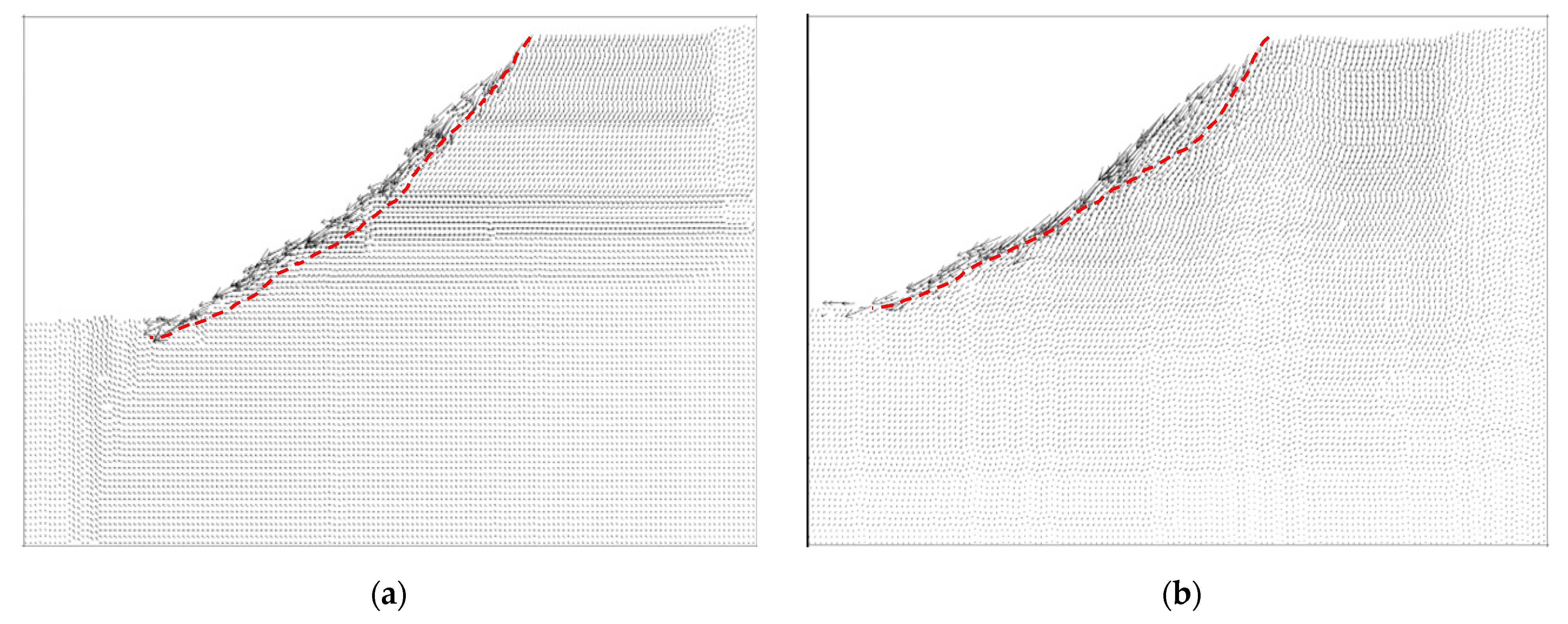
4. Comparison of Failure Modes of RDFN with DFN Models

Figure 7 depicts the failure modes of both the linear and rough-jointed slopes after loading. Both slopes slip as a whole, indicating an arc failure mode. Rock mass upon the red line means the potential sliding part of the slope. From the upper part, it is observed that the linear slope experiences local collapse, consequently reducing its stability in comparison with the rough slope. Additionally, the displacement vector of the slope surface is dense. Consequently, it is believed that a rough-jointed slope is more stable than the linear-jointed slope under equivalent conditions.

Figure 8 illustrates the compression displacement program of linear and rough slopes at various inclination angles after being loaded. As depicted in Figure 8i, the surface displacement distribution of the linear jointed slope displays dense to loose and then a dense trend with an increase in the joint inclination angle from 0° to 90°, as shown in Figure 8i(a–e). Additionally, the slope displacement is tangential to the slope strike. Moreover, the above-mentioned trend of the slope surface displacement is also visible in the failure displacement distribution of rough-jointed slopes, as illustrated in Figure 8ii(a–e). These findings reveal that, while the overall displacement trend of the linear and rough slopes is similar, there are significant differences in the internal displacement of the rock mass, particularly with regards to the position of the through-tension crack and the slip surface distribution. The slip surface of the linear slope, which has a dip angle of 60° is situated in the upper middle section of the slope. Moreover, its starting point is at the highest point of the slope, while its endpoint is at the bottom of the middle step of the slope. The slip surface of a rough slope is located in the middle and lower parts of the slope. Its starting point is also located on the middle step, which is much lower than that of a linear slope. There are visible differences in the position, length, and number of through-tension cracks formed in the failure process of linear and rough slopes. These differences stem from the distribution of formed through-tension cracks.

5. Influence of the Inclination Angle

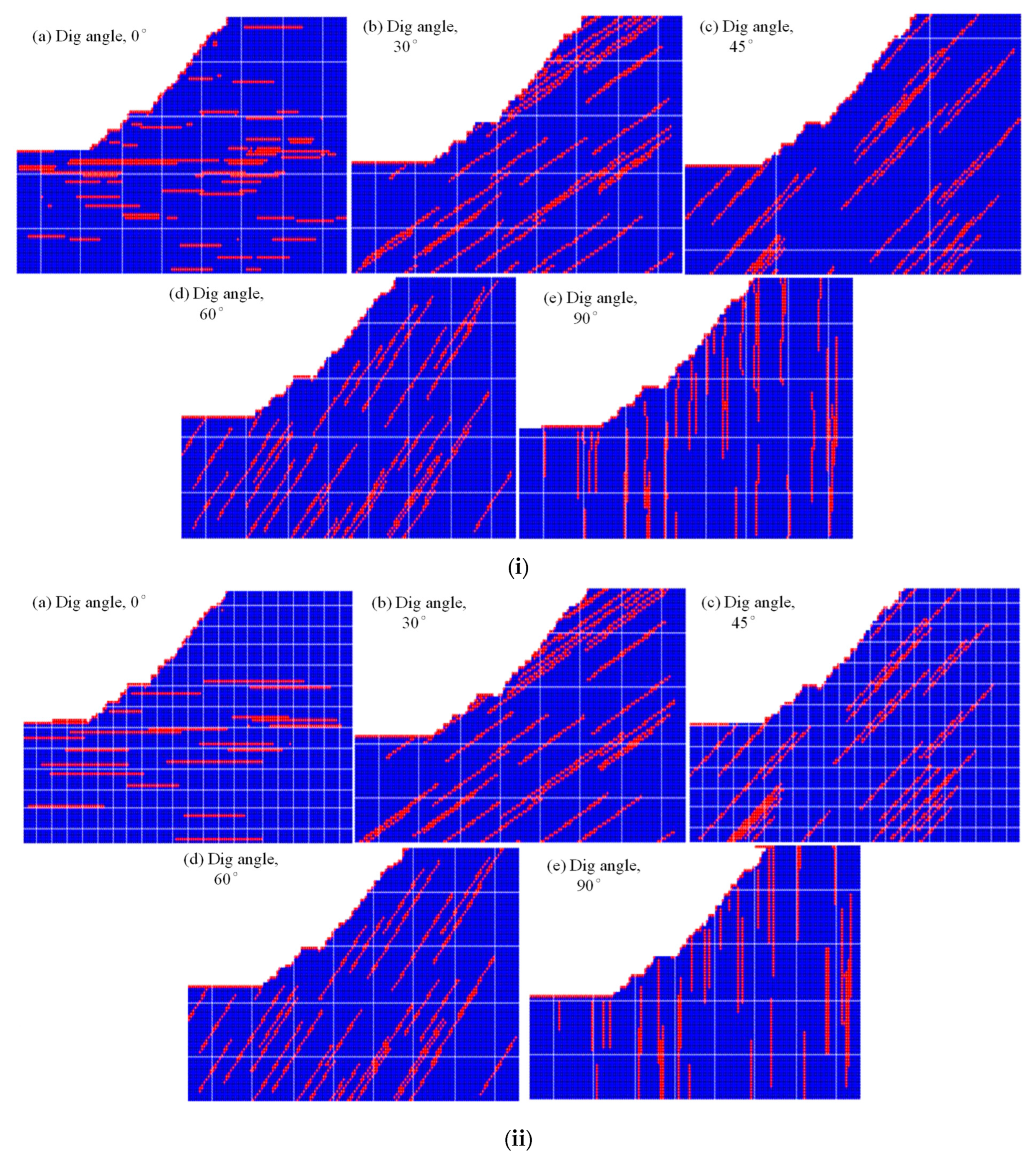
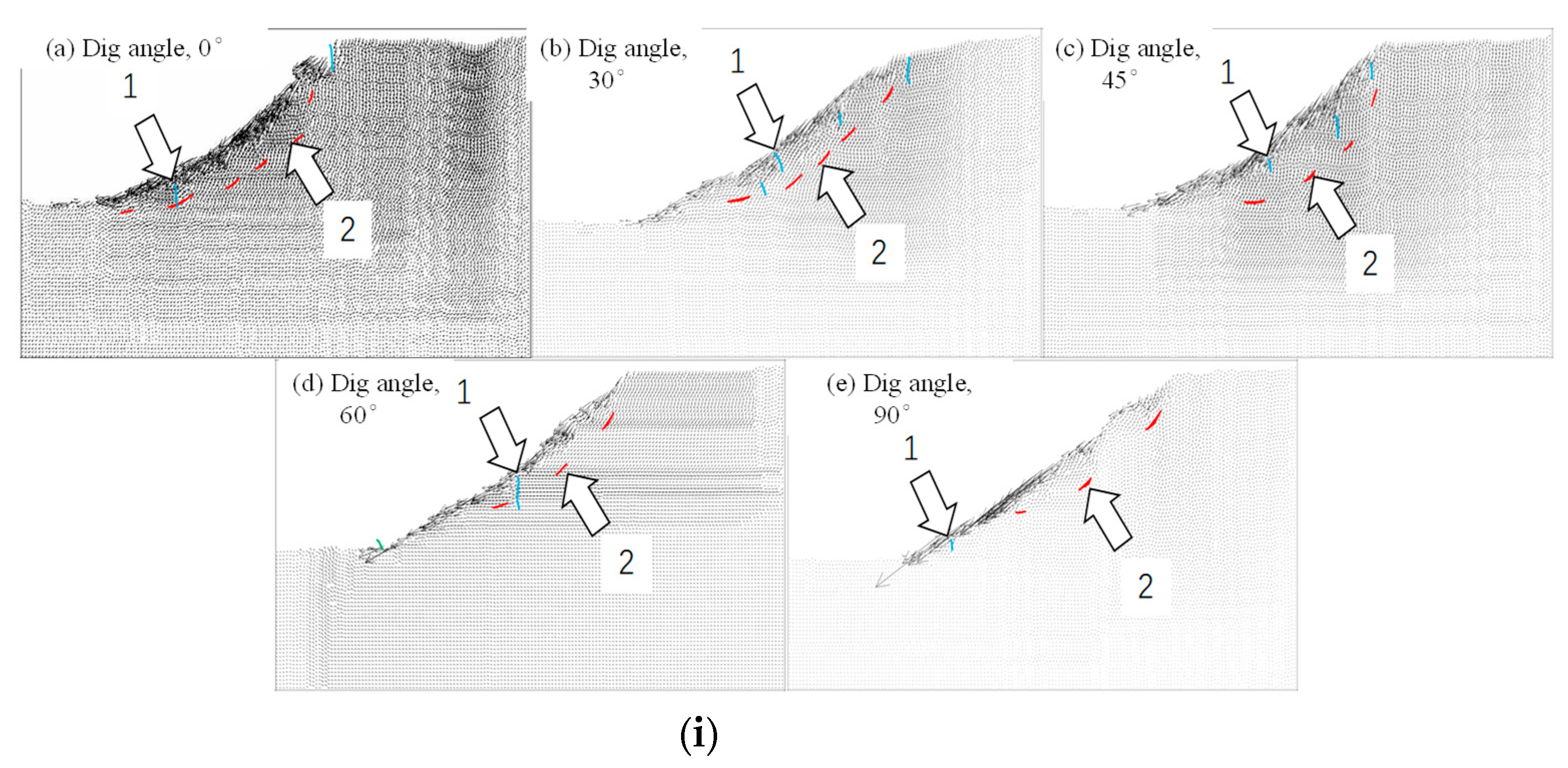
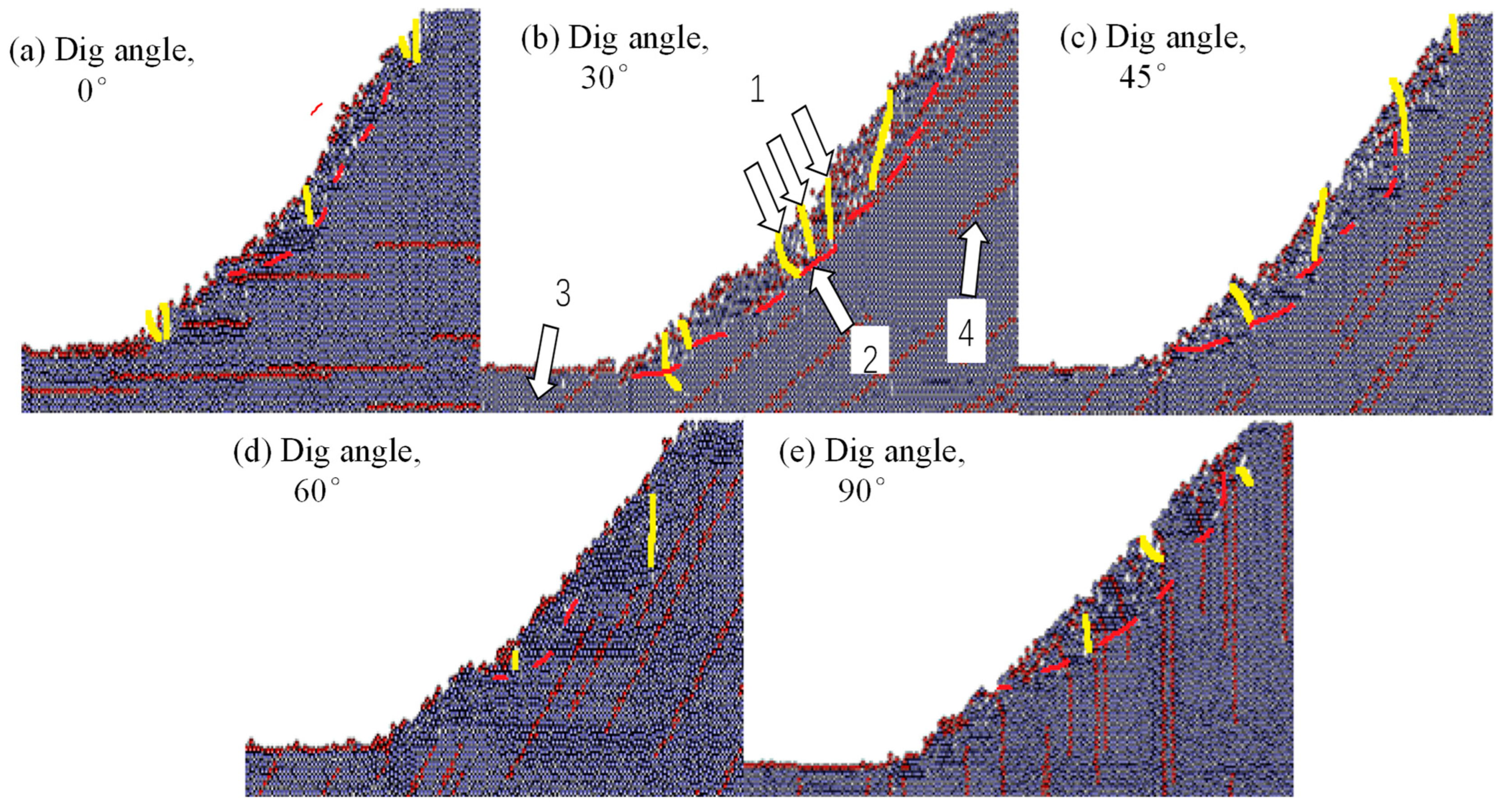
5.1. Failure Modes

The stability of the slope is significantly impacted by the rough joints (Figure 1d), owing to the presence of weak interlayers on the rock slope. Figure 9 illustrates the failure characteristics of rough slopes with joint inclination angles of 0°, 30°, 45°, 60°, and 90° after they are loaded.

As shown in Figure 9a, it slides as a whole, and the surface collapses locally when there is a slope with a 0° joint inclination angle. Some visible cracks are mainly located at the bottom of the top step slope, and the plate of the bottom step is flat. A potential slip surface is formed inside the slope from the lower part of the top step to the upper part. The joints are weak interlayers that lie horizontally; however, the failure destination of the slip line stops at the joint. Chang et al. [22] used the north slope of an open-pit mine as a case study. Through finite element software modeling analysis, he concluded that the failure mode of the layered slope occurred primarily through sliding, with a weak layer being the main failure layer. Additionally, the occurrence of a multi-slide failure indicated that joints had a lower impact on the stability of the self-weight slope when they were not distributed in the upper slope.

As shown in Figure 9b, with regards to the 30° joint inclination angle, the overall slip distance of the slope increases, and multiple tensile cracks appear on its surface after loading. The fractures are distributed mainly in the center and lower sections of the slope, especially in the central part, which traverses multiple joints within the slope. The stability is significantly affected by loading, and a complete slip surface forms within a depth range from the slope’s top to its foot. The angle of the joint inclination is roughly parallel to the surface of the slope, which is considered to be a weak layer compound. In research by Yang et al. [23], the composite slope of a substation site in a rich karst was examined using the strength reduction method and ABAQUS 2021 numerical simulation software. The study also revealed that the composite slope with multiple weak layers first produced a shear fracture and slipped along the weak layer, which may result in a potential fracture surface that is circular arc-shaped. Furthermore, it was found that the stability was mostly affected by the joint dip angle that was parallel to the side slope, which aligned with the numerical simulation results.

The loading failure mode of the slope with a joint inclination angle of 45° (Figure 9c) is similar to that of a slope with a joint inclination angle of 0°. The slope body exhibits the sliding phenomenon and local caving, and tiny cracks that connect the upper and lower parts are also observed. A sliding surface through the lower part of the slope’s top step to the platform at the foot of the slope is also formed. The failure modes of slopes with joint inclination angles of 60° and 90° are also similar, as shown in Figure 9d,e. There are some cracks appearing at the partial top of the slope, and there are local sliding phenomena occurring. However, the starting points of the potential sliding surfaces inside the two slopes differ. The former forms exclusively in the middle of the slope and terminates at the top of the lower step, whereas the latter originates at the top of the slope and terminates at the top of the lower step. As the joint inclination angle increases, the fracture range of the slip surface formed after the internal loading of the slope initially increases, then decreases, and then increases again. At a joint inclination angle of 60°, there is reduced internal fracturing of the slope. According to [24], which uses PFC2D to simulate a typical slope, joint distribution in only the upper part of the slope leads to substantial displacement of the upper rock while the lower part remains unaffected. This suggests that joint distribution has a significant influence on slope stability. Yang et al. [25] presented a mechanical model and failure analysis for a bedding rock slope, along with a numerical simulation of the Shanyang landslide. Research has shown that the slope initially developed a shear-slip zone from the weak parallel structural plane. This zone continued to expand with time and ultimately connected with the tension zone lower down the slope, resulting in slope instability. It has been observed that the shear strength in an unstable bedding slope decreases, owing to the parallel weak structural plane on the slope surface. This observation aligns with the failure state of the simulation slope, which had a joint dip angle of 30° (close to 37° slope angle). A weak joint initiates at the top of the slope and terminates at the slip surface, penetrating the platform beneath the slope.

In engineering, the dip angles of 30°, 45°, and 60° degrees more accurately represent the distribution of joint fluctuation angles in the slope. Most of the dip angles appear as the slope in a composite form. In their study, Liu et al. [26] proposed a generalization of the rock slope model having serrated structural planes with low, medium, and high undulations (with respective undulation angles being 30°, 45°, and 60°). They also established the cumulative damage evolution model of the slope through experiments. Zhong et al. [27] concluded that slope instability follows a specific process, starting from the initiation and development of micro-cracks, followed by expansion and penetration of cracks, and ending with the failure of a slope sliding. The experimental result is consistent with the simulation result, indicating that the difference in joint number has little effect on the final slope failure model. However, the difference in the final failure trace at different joint levels is notable.

Landslide suggests that the slope is influenced by discontinuous stress concentration points during the landslide process. This is due to joints dividing the continuous rock, creating a landslide locking section that primarily consists of rock bridges and supporting arches [28]. The joint units on the slope surface become more severely deformed due to rock rolling and sliding as there are increases in the joint dip angle. The high-stress concentration areas between the joint units are also significantly damaged. This suggests that the slope’s instability is notably influenced by the locking section as the joint inclination angle increases. The variation in the locking section’s shape results in different slope slip lines corresponding to varying joint inclination angles.

Figure 10 illustrates the progression of slope landslides on the engineering site. Several tensile fractures were identified at the measured position. The obtained failure result resembles the simulated slope failure mode, and a slip surface can be observed that formed in the upper part. It shows that the two-dimensional numerical simulation can match some landslide areas on the actual slope, and rock particles accumulate in the lower part after loading, validating the trustworthiness of analyzing the sliding instability of the rock slope structural plane using the PFC2D code.

5.2. Displacement

Figure 11 illustrates the displacement field of the rough slope considering joint inclination angles of 0°, 30°, 45°, 60°, and 90°. It should be noted that the length of the vector arrow reflects the value of its corresponding displacement. The self-weight slope is in a vertical downward compression state after loading when the joint inclination angle is 0°, as shown in Figure 11a. Moreover, the slope displacement vector is tangential to a section of the slip surface, resulting in the sliding of the entire slope. Figure 12 shows the displacement vectors of the slope, which show the distribution of loose bodies, which means the potential slide parts of the slope. Regarding the slope with a joint inclination angle of 30° (Figure 11b), the upper part experiences dense compression displacement, resulting in rapid destruction of the top of the slope through a significant shear slip, leading to the complete destruction of the slope. For a joint inclination angle of 45°, the displacement vector on the slope surface is sparse and parallels the slope surface tangent, as shown in Figure 11c. Nonetheless, the displacement is primarily concentrated in the center of the slope surface, suggesting the slide of the entire slope as a single entity, with the rock mass falling locally in the center of the slope surface. Upon applying a 60° joint inclination angle to the slope model (Figure 11d), the displacement vector along the slope surface is tangential to it, resulting in a dense displacement distribution within the slip surface rupture range. At a joint inclination angle of 90°, shown in Figure 11e, the compression displacement vector remains along the surface tangent, causing the rock on the slope surface to slide down along the slope. 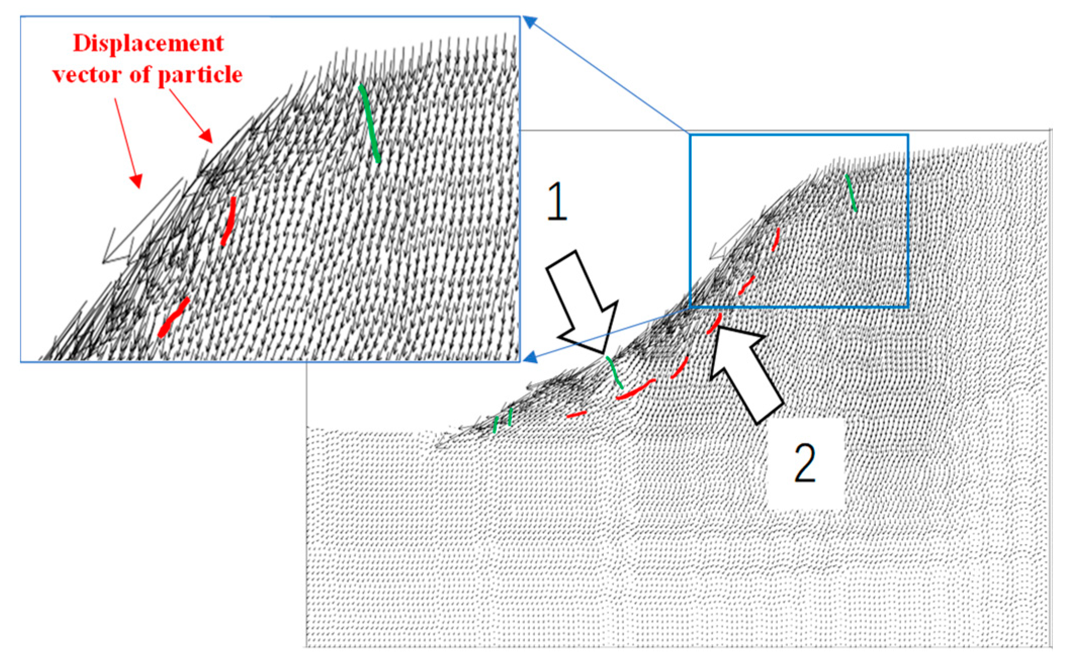The dense displacement vector observed at the base of the slope implies that the sliding rock continually accumulates, resulting in severe displacement.

6. Conclusions

A model for characterizing rough joint traces was proposed by combining the modeling method of a rough discrete fracture network with the RDFN model. This was conducted by utilizing the Fourier transform principle. The model took the fracture dip angle into consideration and utilized digital image recognition technology to develop a mechanical model of a rough slope, using the particle flow discrete element numerical analysis method. This study’s key findings include the following:

• According to this study, a rough slope is more stable than a linear slope for a single fracture inclination angle. Although both slope types show a similar overall displacement trend, they differ significantly in their slip surface and through-tension crack distribution.
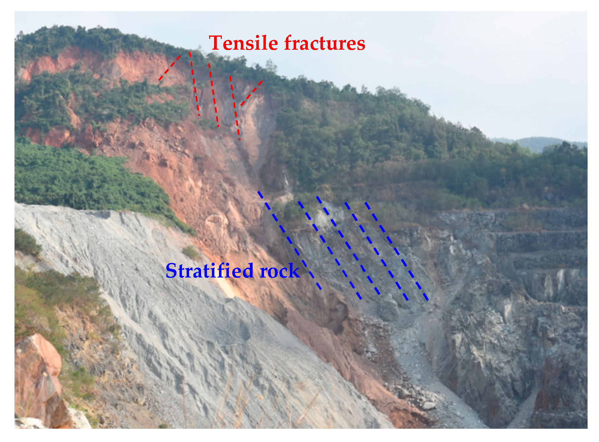
• The vectors of displacement for rough-jointed slopes having inclination angles of 0° and 45° are concentrated at the center of the side slope surface and are tangential to the slope surface. This leads to the sliding of the entire slope, resulting in local caving on the surface. Inclination angles of 30° in the joints produce weaknesses in the structural plane, reducing shear strength and causing a breakdown in the bedding slope. For fracture inclination angles of 60° and 90°, significant displacement of the slope is concentrated in the middle, along with through cracks at the top, which result in local slippage.
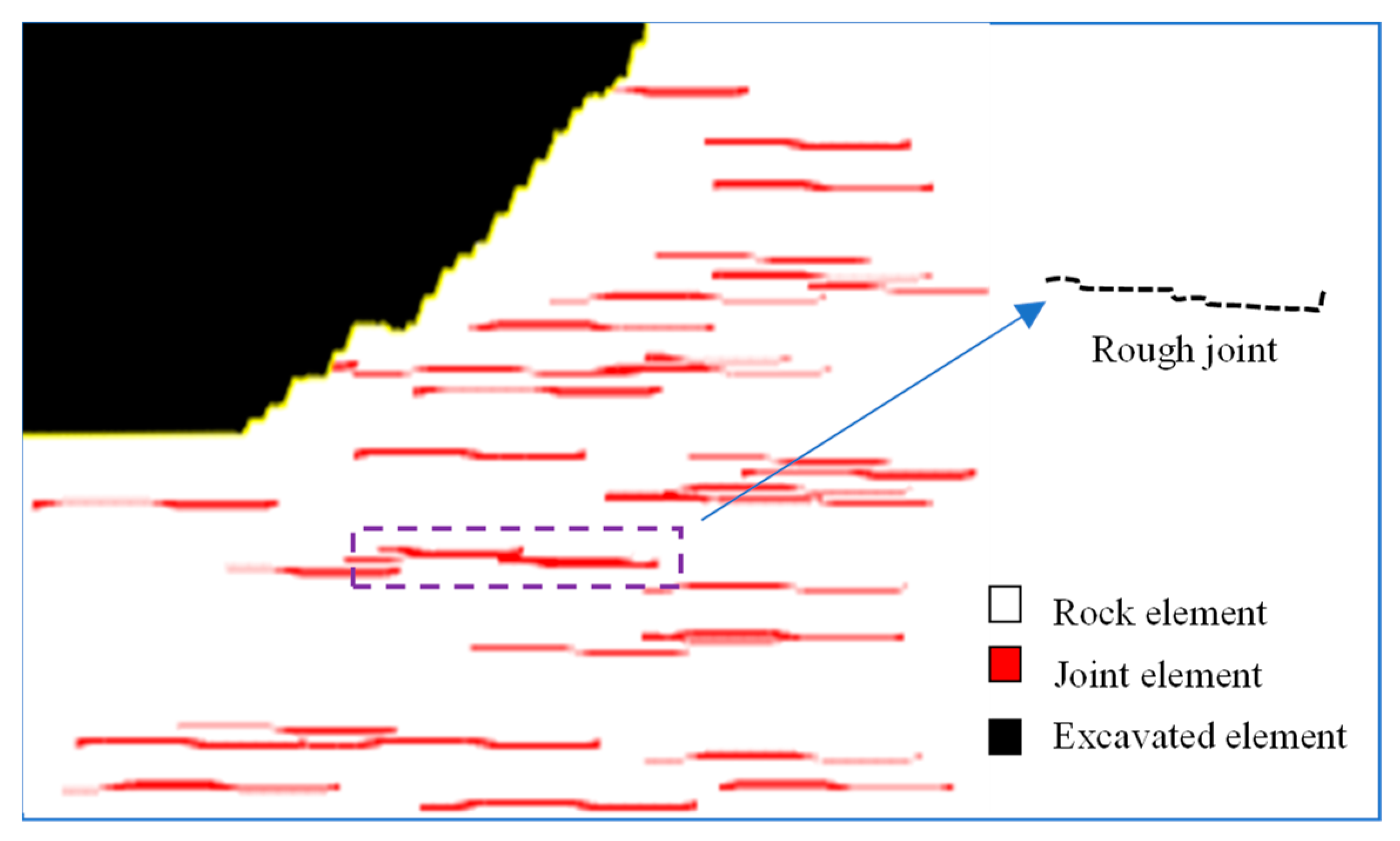
• After comparing simulation results with actual engineering slope failure characteristics and related research, we found that the stability analysis model of rough-jointed rock slopes, based on PFC2D, is closer to the real-world results than the linear-jointed model. This indicates an effective and reliable new method for modeling jointed-rock slopes with complex structures. However, the current modeling method only considers a single fracture distribution mode and a single dip angle, and it needs further optimization to consider multiple dip angles and fracture distributions.

References

- Sellers, E.J.; Klerck, P. Modeling of the effect of discontinuities on the extent of the fracture zone surrounding deep tunnels. Tunneling Undergr. Space Technol. 2000, 15, 463–469. [Google Scholar] [CrossRef]
- Malan, D.F.; Spottiswoode, S.M. Time-dependent fracture zone behavior and seismicity surrounding deep level stopping operations. In Rockburst and Seismicity in Mines; A. A. Balkema: Rotterdam, The Netherlands, 1997; pp. 173–177. [Google Scholar]
- Li, M.; Yue, Z.; Ji, H.; Xiu, Z.; Han, J.; Meng, F. Numerical Analysis of Interbedded Anti-Dip Rock Slopes Based on Discrete Element Modeling: A Case Study. Appl. Sci. 2023, 13, 12583. [Google Scholar] [CrossRef]
- Liu, G.; Zhao, J.; Song, H. Numerical simulation on influence of joint distributions on failures of rock mass. J. China Univ. Min. Technol. 2007, 36, 17–22. [Google Scholar]
- Pariseau, W.G.; Puri, S.; Schmelter, S.C. A new model for effects of impersistent joint sets on rock slope stability. Int. J. Rock Mech. Min. Sci. 2008, 45, 122–131. [Google Scholar] [CrossRef]
- Li, H.; He, Y.; Xu, Q.; Deng, J.; Li, W.; Wei, Y. Detection and segmentation of loess landslides via satellite images: A two-phase framework. Landslides 2022, 19, 673–686. [Google Scholar] [CrossRef]
- Li, H.; He, Y.; Xu, Q.; Deng, J.; Li, W.; Wei, Y.; Zhou, J. Sematic segmentation of loess landslides with STAPLE mask and fully connected conditional random field. Landslides 2023, 20, 367–380. [Google Scholar] [CrossRef]
- Feng, J.; Wang, J.; Cai, M. Udy on the optimization of the slope angle and ability of high eep open pit slope. China Min. Mag. 2005, 14, 45–48. [Google Scholar]
- Gao, Y.; Xiao, S.; Wu, S.; Tian, Q.; Liu, B. Numerical simulation of the deformation and failure characteristics of consequent rock slopes and their stability. Chin. J. Eng. 2015, 37, 1403–1409. [Google Scholar]
- Zhao, W.; Wu, S.; Gao, Y.; Zhou, Y.; Xiao, S. Numerical modeling and mechanical parameters determination of jointed rock mass. Chin. J. Eng. 2015, 37, 1542–1549. [Google Scholar]
- Zhang, Y.; Ren, G.; Chang, W.; Dong, B.; Tang, Y. Probabilistic analysis of stability of jointed rock slope. J. Chengdu Univ. Technol. 2021, 48, 235–241. [Google Scholar]
- Li, D.; Jia, W.; Cheng, X.; Zhao, L.; Zhang, Y.; Yu, P. Stability of stepped sliding of bedding rock slopes with discontinuous joints. Chin. J. Geotech. Eng. 2022, 44, 2125–2134. [Google Scholar]
- Discenza, M.E.; Di Luzio, E.; Martino, S.; Minnillo, M.; Esposito, C. Role of Inherited Tectonic Structures on Gravity-Induced Slope Deformations: Inference from Numerical Modeling on the Luco dei Marsi DSGSD (Central Apennines). Appl. Sci. 2023, 13, 4417. [Google Scholar] [CrossRef]
- Ren, Z.; Chen, C.; Sun, C.; Wang, Y. Dynamic Analysis of the Seismo-Dynamic Response of Anti-Dip Bedding Rock Slopes Using a Three-Dimensional Discrete-Element Method. Appl. Sci. 2022, 12, 4640. [Google Scholar] [CrossRef]
- Nasseri, M.H.B.; Grasselli, G.; Mohanty, B. Fracture toughness and fracture roughness in anisotropic granitic rocks. Rock Mech. Rock Eng. 2010, 43, 403–415. [Google Scholar] [CrossRef]
- Mohd-Nordin, M.M.; Song, K.-I.; Kim, D.; Chang, I. Evolution of joint roughness degradation from cyclic loading and its effect on the elastic wave velocity. Rock Mech. Rock Eng. 2016, 49, 3363–3370. [Google Scholar] [CrossRef]
- Gao, Z.; Wang, S.; Yin, H.; Zhao, Q.; Vladimr, P.; Li, Y. Estimation of Shear Strength Parameters Considering Joint Roughness: A Stability Case Analysis of Bedding Rock Slopes in an Open-Pit Mine. Appl. Sci. 2023, 13, 5730. [Google Scholar] [CrossRef]
- Wang, P.; Liu, C.; Qi, Z.; Liu, Z.; Cai, M. A rough discrete fracture network model for geometrical modeling of jointed rock masses and the anisotropic behaviour. Appl. Sci. 2022, 12, 1720. [Google Scholar] [CrossRef]
- Wu, C.; Bian, K.; Liu, J.; Hu, X.; Gao, Y. Particle discrete element simulation of water absorption and softening effect of heterogeneous rocks. Water Resour. Power 2021, 39, 151–154+150. [Google Scholar]
- Wang, P.; Meifeng, C.; Fenhua, R.; Li, C.; Yang, T. A digital image-based discrete fracture network model and its numerical investigation of direct shear tests. Rock Mech. Rock Eng. 2017, 50, 1801–1816. [Google Scholar] [CrossRef]
- Yoon, J. Application of experimental design and optimization to PFC model calibration in uniaxial compression simulation. Int. J. Rock Mech. Min. Sci. 2007, 44, 871–889. [Google Scholar] [CrossRef]
- Chang, J.; Hou, C.; Zhao, X. Failure mechanism analysis and shape optimization of multi weak layer slope. Mod. Min. 2022, 38, 81–84. [Google Scholar]
- Yang, P.; Li, S.; Chao, W.; Tu, X.; Wang, Y.; Jin, Y.; Zhou, K. Analysis on deformation and failure mechanism of multi-weak layer composite slope in karst region. Sci. Technol. Eng. 2022, 22, 6264–6269. [Google Scholar]
- Zhang, S.; Zhang, Y.; Liang, D. Failure mechanism of inclination joint rock slope based by discrete elements method. J. Water Resour. Archit. Eng. 2022, 20, 19–25+42. [Google Scholar]
- Yang, X.; Lu, Z.; Chen, C.; Sun, C.; Liu, X. Analysis of mechanical model of sliding-bending failure in bedding rock slopes with slab-rent structure. Rock Soil Mech. 2022, 43, 258–566. [Google Scholar]
- Liu, X.; Wang, Y.; Xu, B.; Zhou, X.; Yi, L.; Huang, J.; Wang, Z. Investigation on dynamic response mechanism of slopes with serrated structural planes under degradation of rock mass in hydro-fluctuation belt. Chin. J. Rock Mech. Eng. 2022, 41, 2377–2388. [Google Scholar]
- Zhong, Z.; Huang, D.; Song, Y.; Cen, D. Three-dimensional cracking and coalescence of two spatial-deflection joints in rock-like specimens under uniaxial compression. Int. J. Rock Mech. Min. Sci. 2022, 159, 105196. [Google Scholar] [CrossRef]
- Yin, Y.; Sun, P.; Zhang, M.; Li, B. Mechanism on apparent dip sliding of oblique inclined bedding rockslide at Jiweishan, Chongqing, China. Landslides 2011, 8, 49–65. [Google Scholar] [CrossRef]