Trajectory Tracking Control Design for 4WS Vehicle Based on Particle Swarm Optimization and Phase Plane Analysis

Abstract

With the rapid development of today’s society, the traffic environment has become more and more complex. As an essential part of intelligent vehicles, trajectory tracking has attracted significant attention for its stability and safety. It is prone to poor accuracy and instability in extreme working conditions like high speed. In this paper, a trajectory tracking control strategy to ensure lateral stability at a high speed and low attachment limit conditions is proposed for distributed drive vehicles. The model predictive controller (MPC) was used to control the front wheel angle, and the particle swarm optimization (PSO) algorithm was designed to optimize the MPC control parameters adaptively. The sliding mode controller controls the rear wheel angle, and the vehicle instability degree is judged by analyzing the β − $\dot{\mathsf{\beta }}$ phase plane. The controllers of different instability degrees are designed herein. Finally, a torque divider is designed to consider the actuation anti-slip. The designed controller is verified by Carsim and MATLAB-Simulink co-simulation. The results show that the trajectory tracking controller designed in this paper effectively improves the tracking accuracy under the premise of ensuring stability.

1. Introduction

In today’s society, with the rapid development of intelligent technology, the automobile industry is also developing rapidly. The number of cars is increasing, and the traffic environment is becoming more and more complex. As one of the critical technologies of autonomous driving, trajectory tracking performance should be superior. However, accuracy and vehicle stability need to be ensured during tracking. When the vehicle is on the ground with low adhesion or high speed, it often appears unstable. Ensuring vehicle stability under extreme conditions is a considerable challenge.

Global scholars have conducted in-depth research on autonomous driving path tracking, such as PID control [1], fuzzy control [2], model predictive control (MPC) [3], sliding mode control (SMC) [4], and other methods, to design a tracking controller to track the reference trajectory and ensure tracking accuracy.

MPC uses the current system state, the existing model, and the future control quantities to predict the future output of the system. MPC can solve the problems caused by the conventional path following control and accurately track the target path while considering the dynamic constraints of the vehicle [5,6]. For example, Ye et al. [7] designed a linear model predictive control strategy with soft constraints. The application principle of MPC in vehicle path tracking is to track the target path by establishing a vehicle dynamic model and considering various vehicle dynamic parameters. The front wheel angle or vehicle speed is used as a control variable. The control variables are optimized on a rolling basis, and the feedback correction is kept constant. Although these control algorithms can track the target path, some vehicle dynamic factors are not considered in the controller design process. For example, Tang et al. [8] proposed a trajectory tracking method for uncrewed vehicles that combines model predictive and PID control. Tian et al. [9] designed the MPC control method for the force-driven switching strategy based on the maximum tire lateral force and the zero moment method.

SMC is one of the classical nonlinear control strategies capable of generating discontinuous control and moving the system along a predetermined sliding mode trajectory. Due to the variable structure property of sliding mode control, parameter uncertainties and disturbances do not affect the controller. At the same time, sliding mode control has the advantages of a fast response, a high accuracy, and strong robustness [10]. For example, Liu et al. [11] proposed a lateral control system for active front wheel steering (AFS) and direct yaw moment control (DYC) based on second-order sliding mode control of the super-torsion pendulum, which reduces the chattering phenomenon of conventional sliding mode control. In addition, Wu et al. [12] applied the extended disturbance observer to the sliding mode control so that the steering system had the feedforward compensation function. Nayl et al. [13] designed a new type of continuous sliding surface to reduce chattering. Xing et al. [14] designed a non-singular terminal sliding mode control based on a recurrent neural network structure to improve the trajectory tracking performance.

Compared with the traditional front wheel steering vehicle, the four-wheel steering technology has the vehicle’s front and rear four wheels participate in the steering motion together, thus improving the handling stability of the vehicle in high-speed steering and the maneuvering flexibility in low-speed turning. Depending on its actuators, four-wheel steering technology can be divided into four-wheel active steering (4WAS) and four-wheel independent steering (4WIS). In these technologies, the driver controls the front wheel steering of 4WS, according to the road conditions, and the rear wheel angle is determined by the vehicle state and the input of the front wheel driver through the controller. However, in 4WAS and 4WIS, the wheel angle is obtained by comprehensive judgment based on the driver’s steering input and the vehicle state input to the controller. The first incarnation of 4WS technology dates back to 1980, when it was introduced in Japan. Compared with 4WAS and 4WIS, 4WS is one of the most widely studied and applied technologies, and many control strategies and methods are based on 4WS technology [15,16,17]. Chen et al. [18] used a linearization method to simplify the 3-DOF nonlinear vehicle model of 4WS moderately, retaining the coupling characteristics of the vehicle model in terms of driving/braking and the wheel angle, and designed a decoupler of the 4WS vehicle system to realize the decoupling control of the vehicle. Marino [19] designed a dynamic decoupling controller for 4WS vehicles, which is also a simplification of the 3-DOF nonlinear vehicle model. Unlike this, the decoupling controller does not require the observation or estimation of the lateral velocity but implements the decoupling of the yaw velocity and the lateral velocity through the input of additional front wheel angle and rear wheel angle.

In addition, many studies have been conducted by other scholars. Hima S et al. [20] designed a trajectory tracking controller based on horizontal and vertical decoupling. The nonlinear problem in the model is alleviated by PID control with feedback and adaptive control. Y. Jeong et al. [21] and H. Yang [22] et al. designed trajectory tracking controllers for four-wheel steering vehicles, which improved the tracking accuracy compared to front wheel steering vehicles but did not consider the vehicle speed or road conditions. Some other researchers have designed trajectory tracking based on predictive tracking theory and have designed more accurate trajectory tracking simulators by optimizing the preview or direction control [23,24,25]. For example, Chen et al. [26] proposed a kind of driver direction control model based on trajectory prediction on the basis of the assumption that the driver has the ability to predict the vehicle trajectory. We have analyzed the literature cited above as shown in

Table 1. Literature review and analysis.

Ref.	Approach	Limitations
Tang [8]	The kinematic MPC is used to deal with the road curvature disturbance, the yaw rate PID feedback control is used to eliminate the uncertainty and modeling error, and the vehicle sideslip angle compensator is used to correct the kinematic model prediction. This strategy improves the control accuracy and ensures vehicle stability.	The control parameters, such as Q and R, in the MPC controller are fixed values, therefore, adaptive control cannot be achieved.
Liu [11]	A force-driven switched MPC path following the control strategy is proposed to coordinate the active front wheel steering and external yaw torques. This strategy improves the control accuracy and ensures the stability of the vehicle.	This paper only considers the trajectory tracking and stability control under constant speed, however, in practice, the vehicle speed is variable, and the adaptive control of the vehicle speed is not realized.
Chen [18]	Quasi-linearization techniques are used to simplify the vehicle model, which preserves the inherent coupling effects between the longitudinal acceleration/braking force, steering angle, and vehicle state. Based on this model, an input-output decoupling controller is proposed.	The complexity of the control strategies might pose challenges in real-world implementation and calibration.
Hima S [20]	In this paper, the decoupling design method of the longitudinal and lateral controllers is used. For the longitudinal controller, the proportion containing the feedforward term is used. On the other hand, an adaptive backstepping method is used in the lateral case to deal with the nonlinearity and parameter uncertainty of the model.	The influence of vehicle speed and road conditions on vehicle stability is not considered, and different control strategies should be divided for different stability degrees.

.

In this paper, a trajectory tracking control algorithm based on distributed driving is designed for 4WS vehicles. Based on the distributed drive stability control strategy, it gives full play to the advantages of the distributed drive chassis system, solves the problem of vehicle trajectory tracking under extreme working conditions, and realizes the design of a trajectory tracking control algorithm for multi-objective coordinated control. The specific contributions are as follows:

(1) The particle swarm optimization (PSO) algorithm is used to optimize the MPC controller. Q and R are the primary weight coefficients in the MPC control process. The PSO algorithm is used to optimize and adjust the weighting coefficients, the fitness function is iteratively reduced until the iteration number requirements are met, and the optimization is stopped to realize the goal of adaptive optimization of the MPC control parameters.

(2) In the sliding mode controller of the rear wheel angle, a sliding mode surface referring to the PID controller is designed, and factors such as driving anti-slip are considered in the torque distributor so that the torque distribution of each wheel is more reasonable.

(3) An improved phase plane stability judgment method is designed to judge the instability degree of the vehicle in real-time, and different partition controllers are designed according to the instability degree to control the additional yawing moment. It is verified that the tracking accuracy can be improved while ensuring the vehicle’s stability.

2. 2-DOF Vehicle Dynamics Model and Ideal Reference Model

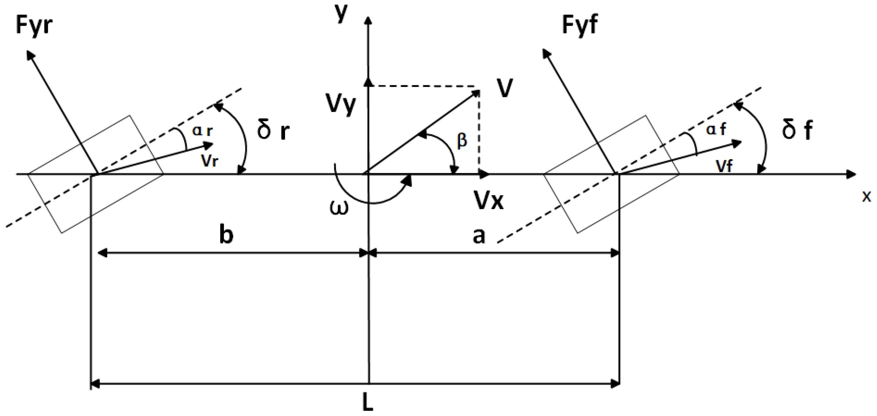
Due to the simplification of the vehicle structure, the 2-DOF dynamics model is widely used to analyze vehicle-related problems. In the 2-DOF model, the left and right wheels of the vehicle are considered as a whole, as shown in Figure 1 below. The distributed drive vehicle can independently control the torque of the four steering wheels to achieve four-wheel steering control. In addition, controlling the direct yaw moment is necessary to ensure stability. Therefore, the 2-DOF model can characterize the lateral motion of the vehicle and is suitable for this study [27].

Based on the 2-DOF model in the figure, the longitudinal velocity of the car along the x-axis direction is assumed to be constant, and only the lateral motion of the vehicle on the y-axis and the yaw motion around the z-axis are considered. In order to obtain the ideal front wheel angle, the influence of air resistance, suspension, and rear wheel angle is not considered.

The lateral motion of the vehicle is shown in Equation (1).

$$\mathrm{m}(\stackrel{·}{v_y}+v_x\omega )=F_{yf}\cos {\delta }_f+F_{yr}$$

(1)

The yaw motion of the vehicle is shown in Equation (2).

$$I_z\stackrel{·}{\omega }=a{F}_{yf}\cos {\delta }_f-b{F}_{yr}$$

(2)

where ${\mathrm{F}}_{\mathrm{y}\mathrm{f}}$ and ${\mathrm{F}}_{\mathrm{y}\mathrm{r}}$ are the lateral reaction forces of the ground to the front and rear wheels, respectively. a and b are the distances between the center of the mass of the vehicle and the front and rear axles, respectively. ${\mathsf{\delta }}_{\mathrm{f}}$ is the front wheel angle; ω is the car’s yaw rate; ${\mathrm{I}}_{\mathrm{z}}$ is the moment of inertia of the vehicle around the z-axis; and ${\mathrm{v}}_{\mathrm{x}}$ and ${\mathrm{v}}_{\mathrm{y}}$ are the forward and lateral speeds of the vehicle, respectively.

In the classic 2-DOF vehicle model, the longitudinal force of the tire is usually ignored when analyzing the lateral dynamics. However, in the research of MPC trajectory tracking control, the front wheel angle is assumed to be small for calculating the speed, and the influence of the longitudinal force of the tire is also ignored to simplify the model. Therefore, in this paper, the front wheel angle is assumed to be a slight angle, and Equations (1) and (2) can be deduced.

$$\left\{\begin{array}{l}{\displaystyle \sum F=F_{yf}\cos {\delta }_f+F_{yr}=F_{yf}+F_{yr}=k_1{\alpha }_f+k_2{\alpha }_r}\\ {\displaystyle \sum M=a{F}_{yf}\cos {\delta }_f-b{F}_{yr}=a{k}_1{\alpha }_f-b{k}_2{\alpha }_r}\end{array}\right.$$

(3)

where ${\mathsf{\alpha }}_{\mathrm{f}}$ and ${\mathsf{\alpha }}_{\mathrm{r}}$ are the lateral deflection angles of the front and rear wheels, respectively; ${\mathrm{k}}_1$ and ${\mathrm{k}}_2$ are the lateral deflection stiffness of the front and rear axes.

Equation (3) can be rewritten into a differential motion equation after derivation, as shown in Equation (4).

$$\left\{\begin{array}{l}m(\stackrel{··}{v_y}+\omega v_x)=(k_1+k_2)\beta +\frac{1}{v_x}(a{k}_1-b{k}_2)\omega -k_1{\delta }_f\\ I_z\stackrel{·}{\omega }=(a{k}_1+b{k}_2)\beta +\frac{1}{v_x}(a^2{k}_1-b^2{k}_2)\omega -a{k}_1{\delta }_f\end{array}\right.$$

(4)

where β is the lateral deflection angle of the center of mass.

The ideal reference model is used to describe the lateral motion of the vehicle at a steady state when the front wheel angle is minimal and can be neglected. In this case, the yaw rate is the ideal yaw rate, and, at the same time, the ideal center of mass lateral angle can be calculated. Since the front wheel angle is ignored, the vehicle is performing a uniform circular motion, therefore, $\dot{{\mathrm{v}}_{\mathrm{y}}}$ and $\dot{\mathsf{\omega }}$ are zero, and joint Equation (4) can be obtained as follows:

$$\left\{\begin{array}{l}m\omega v_x=\beta (k_2+k_1)-k_1{\delta }_f+\omega /v_x(a{k}_1-b{k}_2)\\ 0=\beta (a{k}_1+b{k}_2)-a{k}_1{\delta }_f+\omega /v_x(a^2{k}_1-b^2{k}_2)\end{array}\right.$$

(5)

The stable yaw rate, with respect to ${\mathrm{v}}_{\mathrm{x}}$ and ${\mathsf{\delta }}_{\mathrm{f}}$, can be determined as follows:

$${\omega }_d=\frac{{\delta }_f{v}_x}{L+\frac{\mathrm{m}{v_x}^2(a{k}_1-b{k}_2)}{L{k}_1{k}_2}}$$

(6)

Due to the influence of the road adhesion coefficient μ, the vehicle should meet ${\mathrm{a}}_{\mathrm{y}}\le \mathsf{\mu }\mathrm{g}$ while driving, and the motion state of the vehicle should meet the following requirements:

$$a_y=\omega v_x+\stackrel{•}{v_x}\tan \beta +\frac{v_x\beta }{\sqrt{1+\tan \beta }}$$

(7)

When the vehicle is in steady state, the value of β is negligible, therefore, ${\mathrm{a}}_{\mathrm{y}}{=\mathsf{\omega }}_{\mathrm{r}}{\mathrm{v}}_{\mathrm{x}}$ is desirable. Since many influencing factors exist in practice, a 15% stability margin can be processed. Taking the ideal centroid sideslip angle to be zero, the desired ideal yaw rate and centroid sideslip angle can be obtained as follows:

$$\left\{\begin{array}{l}{\omega }_d=\min \left\{\right|{\omega }_d|,|\frac{0.85\mu g}{v_x}\left|\right\}\mathrm{sgn}({\delta }_f)\\ {\beta }_d=0\end{array}\right.$$

(8)

where L is the front and rear wheelbase; μ is the road adhesion coefficient; ${\mathsf{\omega }}_{\mathrm{r}}$ is the actual yaw rate; ${\mathsf{\omega }}_{\mathrm{d}}$ and ${\mathsf{\beta }}_{\mathrm{d}}$ are the ideal yaw rate and the centroid, respectively; and g is the acceleration of gravity.

3. Design of Trajectory Tracking Control System

Figure 2 shows a frame diagram of the proposed trajectory tracking control system. The vehicle obtains the target road information and the real-time state parameters of the vehicle through the planning layer, which are input into the MPC, and the ideal front wheel angle is obtained by PSO optimization calculation. At the same time, the ideal yaw rate, the actual yaw rate, and the actual yaw angle are obtained by the ideal reference model as the control input of the sliding mode controller. The stability controller is designed based on the sliding mode control theory, the rear wheel angle is calculated, and the additional yaw moment based on the yaw rate and the yaw angle of the center of mass is obtained. In the stability controller of the phase plane method, the instability degree of the vehicle is identified according to the $\mathsf{\beta }-\dot{\mathsf{\beta }}$ phase plane of the vehicle, and the additional yaw moment ΔM is calculated according to the designed partition controller. PID control is used to track the target vehicle speed and solve the driving force ${\mathrm{F}}_{\mathrm{t}}$. Finally, a torque distributor is designed to distribute the torque of the in-wheel motor of each wheel according to ΔM and ${\mathrm{F}}_{\mathrm{t}}$ and considering the driving anti-slip and other factors.

3.1. Design of MPC Controller

When tracking the reference path, the vehicle has the following relationship:

$$\left\{\begin{array}{l}\dot{\phi }=\omega \\ \dot{Y}=v_x\phi +v_y\end{array}\right.$$

(9)

where φ is the actual heading angle of the vehicle and Y is the lateral position of the vehicle in the geodetic coordinate system.

Combined with Equations (4) and (9), it can be transformed into the form of state space equation, where the state quantity is $\mathrm{x}=[{\mathrm{v}}_{\mathrm{y}},\mathsf{\omega },\mathsf{\phi },\mathrm{Y}]$, the control quantity is $\mathsf{\mu }={\mathsf{\delta }}_{\mathrm{f}}$, the output quantity is $\mathrm{y}=[\mathsf{\phi },\mathrm{Y}]$, and the state space equation is Equation (10).

$$\left\{\begin{array}{l}\dot{x}=Ax+Bu\\ y=Cx+Du\end{array}\right.$$

(10)

where $\mathrm{A}=\left[\begin{array}{cccc}\frac{{\mathrm{k}}_1{+\mathrm{k}}_2}{{\mathrm{mv}}_{\mathrm{x}}}& \frac{{(\mathrm{ak}}_1{-\mathrm{bk}}_2)}{{\mathrm{mv}}_{\mathrm{x}}}{-\mathrm{v}}_{\mathrm{x}}& 0& 0\\ \frac{{(\mathrm{ak}}_1{-\mathrm{bk}}_2)}{{\mathrm{I}}_{\mathrm{z}}{\mathrm{v}}_{\mathrm{x}}}& \frac{{(\mathrm{a}}^2{\mathrm{k}}_1{+\mathrm{b}}^2{\mathrm{k}}_2)}{{\mathrm{I}}_{\mathrm{z}}{\mathrm{v}}_{\mathrm{x}}}& 0& 0\\ 0& 1& 0& 0\\ 1& 0& {\mathrm{v}}_{\mathrm{x}}& 0\end{array}\right]$; $\mathrm{B}=\left[\begin{array}{c}-\frac{{\mathrm{k}}_1}{\mathrm{m}}\\ -\frac{{\mathrm{ak}}_1}{{\mathrm{I}}_{\mathrm{z}}}\\ 0\\ 0\end{array}\right]$; $\mathrm{C}=\left[\begin{array}{cccc}\begin{array}{l}0\\ 0\end{array}& \begin{array}{l}0\\ 0\end{array}& \begin{array}{l}1\\ 1\end{array}& \begin{array}{l}0\\ 0\end{array}\end{array}\right]$; $\mathrm{D}={\left[0\right]}_{2*1}$.

The optimal control sequence for MPC controllers is solved in the prediction time domain by solving an optimization problem that satisfies the objective function and various constraints. The first element of this control sequence is taken as the actual control quantity of the controlled plant, and the above solution process is repeated to realize the continuous control of the controlled plant. In order to apply the model to the design of the MPC controllers, the state space equations need to be discretized. The change speed of the control variable in the MPC controller dramatically influences the actual controlled system, so it is necessary to restrict the increment of the control quantity and transform Equation (10).

$$\left\{\begin{array}{l}{\zeta }_{k+1}=A_1{\xi }_k+B_1\Delta U_k\\ {\eta }_k=C_1{\xi }_k\end{array}\right.$$

(11)

where the new state quantity is ${\mathsf{\xi }}_{\mathrm{k}}=\left[\begin{array}{l}{\tilde{\mathrm{x}}}_{\mathrm{k}-1}\\ {\tilde{\mathrm{u}}}_{\mathrm{k}}\end{array}\right]$, and the change in the control quantity at each time compared with the previous time is called $\mathsf{\Delta }{U}_k$, ${\mathrm{A}}_1=\left[\begin{array}{cc}\mathrm{A}& \mathrm{B}\\ 0_{\mathrm{Nu}*\mathrm{Nx}}& {\mathrm{I}}_{\mathrm{Nu}*\mathrm{Nx}}\end{array}\right]$; ${\mathrm{B}}_1=\left[\begin{array}{l}\mathrm{B}\\ {\mathrm{I}}_{\mathrm{Nu}*\mathrm{Nu}}\end{array}\right]$; ${\mathrm{C}}_1{=[\mathrm{I}}_{\mathrm{Nx}*\mathrm{Nx}}{,0}_{\mathrm{Nx}*\mathrm{Nu}}]$; $Nx$ is the number of states; and $Nu$ is the number of control quantities.

The system is assumed to be observable and controllable, and the sequence of control quantities is as follows:

$$\Delta U={[\Delta u(k),\Delta u(k+1),\dots ,\Delta u(k+Nc-1)]}^T$$

(12)

The reference point of the reference path is the column vector of $\mathrm{N}\mathrm{p}\mathrm{*}1$, and the expression is as follows:

$$Y_{ref}={[y_{ref}(k+1),y_{ref}(k+2),\dots ,y_{ref}(k+Np)]}^T$$

(13)

Assume that the prediction vector Y of MPC is given by the following:

$$Y={[X(k+1),X(k+2),\dots ,X(k+Np)]}^T$$

(14)

The objective function needs to add the deviation of the system state quantity and the size of the control quantity as the optimization objective to ensure that the uncrewed vehicle can track the reference path quickly and smoothly. The objective function is a quadratic optimization problem, which can be expressed as follows:

$$J={(Y-Y_{ref})}^T\mathrm{Q}(Y-Y_{ref})+\Delta {\mathrm{U}}^{T}R\Delta \mathrm{U}$$

(15)

where Q and R are the weight matrices; and Np and Nc are the prediction and control time domains of MPC, respectively.

This study mainly considers the control quantity limit constraint and the control increment constraint in the control process, and the control quantity limit constraint is as follows:

$$\left\{\begin{array}{l}{u}_{\min }(t+k)\le u(t+k)\le u_{\max }(t+k),k=0,1,\dots ,Nc-1\\ \Delta u_{\min }(t+k)\le \Delta u(t+k)\le \Delta u_{\max }(t+k),k=0,1,\dots ,Nc-1\end{array}\right.$$

(16)

In this paper, the front wheel angle is constrained, the constraint range is [−0.44,0.44], the incremental constraint range is [−0.005,0.005], and the unit is deg.

The quadratic optimization problem can be solved by finding the front wheel steering angle under the constraints. After calculating the optimal steering angle sequence, only the first output controls the system’s next sampling time. The optimization problem is solved recursively within each step.

The Particle Swarm Optimization Algorithm Optimizes the Controller Parameters

Particle swarm optimization (PSO) is an algorithm based on bionics proposed by American scholars Kennedy and Eberhart. The concept of PSO comes from the study of bird foraging behavior. Birds adjust their behavior by sharing their own existing information and combining the information shared by other individuals in the group so that they are in a favorable position to find food and avoid natural enemies. PSO has the advantages of a fast convergence speed, few parameters, and easy implementation (for high-dimensional optimization problems, it converges to the optimal solution faster than other algorithms); however, it also has the problem of falling into local optimal solutions, so it depends on a good initialization.

Assuming a search in a d-dimensional space, particle optimization is equivalent to updating the position and velocity of the individual extreme value and the group extreme value of the particle in each iteration, as shown in Equation (17).

$$\left\{\begin{array}{l}{x}_{t+1}=x_t+v_{t+1}\\ v_{t+1}={\omega }_n{v}_t+c_1{r}_1(P_t-x_t)+c_2{r}_2(G_t-x_t)\end{array}\right.$$

(17)

where ${\mathrm{x}=(\mathrm{x}}_1{,\mathrm{x}}_2,\dots {,\mathrm{x}}_{\mathrm{n}})$ represents the position of the particle; ${\mathrm{v}=(\mathrm{v}}_1{,\mathrm{v}}_2,\dots {,\mathrm{v}}_{\mathrm{n}})$ represents the velocity of the particle; ${\mathsf{\omega }}_{\mathrm{n}}$ is the inertia factor; $c_1,c_2$ are the acceleration constant; ${\mathrm{r}}_1$ and ${\mathrm{r}}_2$ are random number between 0 and 1; ${\mathrm{P}}_{\mathrm{t}}$ is the best position of the particle searched so far; and ${\mathrm{G}}_{\mathrm{t}}$ is the optimal position that PSO has searched so far.

The PSO algorithm needs a judgment condition to determine whether the optimal result is achieved. It usually takes the preset maximum number of iterations or the lower limit of the fitness value as the termination condition. The selection of different fitness functions often determines the convergence speed of the PSO and the probability of the optimal solution. Figure 3 shows a flowchart of the optimization process of the PSO algorithm. The commonly used fitness function is as follows: The integral time absolute error (ITAE) criterion is used because the control system designed by the ITAE index has a better dynamic performance and slight overshoot. In this paper, the sum of the ITAE of lateral deviation, heading deviation ${\mathsf{\phi }}_{\mathrm{error}}$, and steering input $\mathrm{u}$ is applied as the performance index function of PSO MPC, as shown in Equation (18).

$$ITAE={\omega }_1{\displaystyle {\int }_0^{\infty }{\mathrm{t}|\mathrm{Y}}_{error}(t)|dt+}{\omega }_2{\displaystyle {\int }_0^{\infty }\mathrm{t}|{\phi }_{error}(t)|dt+}{\omega }_3{\displaystyle {\int }_0^{\infty }\mathrm{t}|u(t)|dt}$$

(18)

where ${\mathrm{Y}}_{\mathrm{error}}{\left(\mathrm{t}\right), \mathsf{\phi }}_{\mathrm{error}}\left(\mathrm{t}\right) \mathrm{and} \mathrm{u}\left(\mathrm{t}\right)$ represents the lateral deviation, heading deviation, and steering input at time t; and ${\mathsf{\omega }}_1{, \mathsf{\omega }}_2{ \mathrm{and} \mathsf{\omega }}_3$ are the weighting coefficients of each item, which determine the proportion of ITAE index of ${\mathrm{Y}}_{\mathrm{error}}{\left(\mathrm{t}\right),\mathsf{\phi }}_{\mathrm{error}}\left(\mathrm{t}\right) \mathrm{and} \mathrm{u}\left(\mathrm{t}\right)$ in the performance function, respectively.

The velocity update of the traditional PSO optimization algorithm is shown in Equation (17). The particle swarm will only reach the optimal position if the inertia factor parameter is manageable. They set the inertia factor parameter to be too small, leading to a slow convergence speed. The following improvements will be made to the inertia factor: In the early stage of optimization, choosing a more significant factor can enhance the global search ability of the particle and then find the optimal point position faster. In the later stage of the algorithm, a smaller factor is more conducive to improving the convergence speed and local search ability. Therefore, the inertia factor is set as follows in this paper:

$${\omega }_{\mathrm{n}}(t)=0.9-0.5(t-Maxlter)$$

(19)

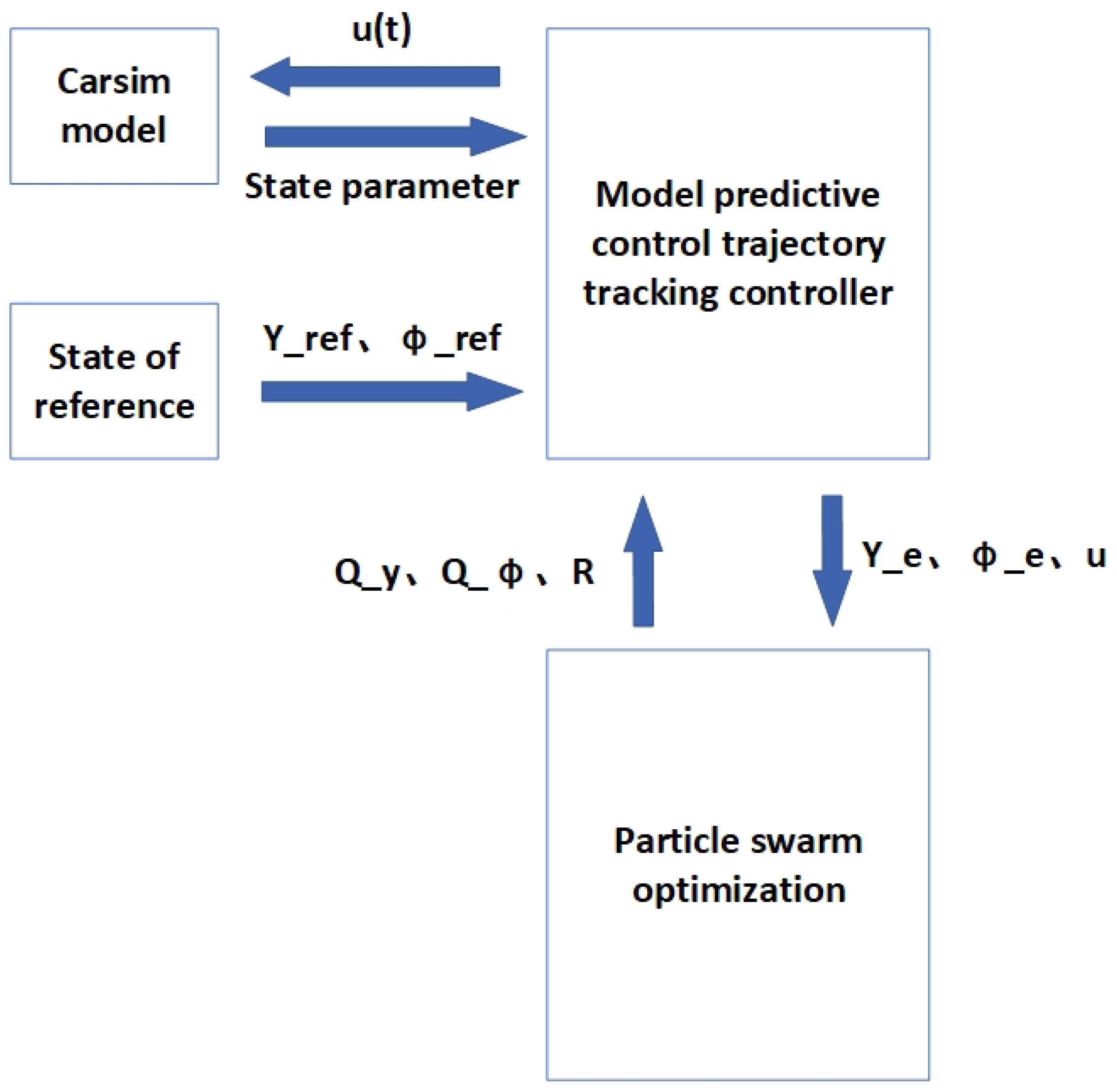
The PSO algorithm is used to optimize the MPC controller. The primary weight coefficients are in the MPC control process. The PSO algorithm is used to optimize and modify the weighting coefficient, and the iterative optimization is used to reduce the ITAE index. Until the iteration number is satisfied, the optimization is stopped in order to realize the purpose of adaptive optimization of the MPC control parameters. Figure 4 shows the process diagram of the PSO algorithm used to implement the optimal design of the MPC parameters.

In the particle swarm optimization (PSO) algorithm, the timeliness and the quasi-certainty of the optimization results are ensured. The initial population number N is set as 30. The maximum iteration number Maxlter is 100. The position limit is 0.5~2. The speed limit is −0.2~0.2. The acceleration constants c1 and c2 are 0.5 and 0.4, respectively. The inertia factor is given in Equation (19).

3.2. Design of the Sliding Controller

When the vehicle is running, the control system can control the steering and longitudinal force of the tire in real time to make the vehicle state meet the ideal reference model. By solving the ideal two-degree-of-freedom model, the center of mass sideslip angle and yaw rate can be used as the control target of stability. Based on Equation (4), the 2-DOF nonlinear model can be obtained as follows [28]:

$$\left\{\begin{array}{l}\stackrel{•}{\beta }=\frac{k_1+k_2}{m{v}_x}\beta +(\frac{a{k}_1-b{k}_2}{m{v_x}^2}-1)\omega -\frac{k_1}{m{v}_x}{\delta }_f-\frac{k_2}{m{v}_x}{\delta }_r\\ \stackrel{•}{\omega }=\frac{a{k}_1-b{k}_2}{I_z}\beta +\frac{a^2{k}_1+b^2{k}_2}{I_z{v}_x}\omega -\frac{a{k}_1}{I_z}{\delta }_f+\frac{b{k}_2}{I_z}{\delta }_r+\frac{1}{I_z}\Delta M\end{array}\right.$$

(20)

Taking the difference between the center of mass sideslip angle and yaw rate and their respective ideal values as the control quantities of the sliding mode control, the control error is as follows:

$$\mathrm{e}=\left[\begin{array}{l}{e}_1\\ e_2\end{array}\right]=\left[\begin{array}{l}\beta -{\beta }_d\\ \omega -{\omega }_d\end{array}\right]$$

(21)

In order to improve the anti-interference ability and accuracy of the system, this paper designs the sliding mode surface concerning PID control, as shown in Equation (22).

$$S={\lambda }_{1}e+{\lambda }_2\stackrel{•}{e}+{\lambda }_3{\displaystyle {\int }_o^{t}e}dt=\left[\begin{array}{l}{\lambda }_{11}\\ {\lambda }_{12}\end{array}\right]\left[\begin{array}{l}{e}_1\\ e_2\end{array}\right]+\left[\begin{array}{l}{\lambda }_{21}\\ {\lambda }_{22}\end{array}\right]\left[\begin{array}{l}\stackrel{•}{e_1}\\ \stackrel{•}{e_2}\end{array}\right]+\left[\begin{array}{l}{\lambda }_{31}\\ {\lambda }_{32}\end{array}\right]\left[\begin{array}{l}{\displaystyle {\int }_o^t{e}_1}dt\\ {\displaystyle {\int }_o^t{e}_2}dt\end{array}\right]$$

(22)

In order to implement the dynamic sliding mode, the exponential reaching rate is used as follows:

$$\stackrel{•}{S}=-\epsilon \mathrm{sgn}(S)-KS=-\left[\begin{array}{cc}{\epsilon }_1& 0\\ 0& {\epsilon }_2\end{array}\right]\left[\begin{array}{c}\mathrm{sgn}(S_1)\\ \mathrm{sgn}(S_2)\end{array}\right]-\left[\begin{array}{cc}{K}_1& 0\\ 0& K_2\end{array}\right]\left[\begin{array}{l}{S}_1\\ S_2\end{array}\right]$$

(23)

In the above equation, ε is the sliding mode boundary layer thickness and K is the reaching rate index, where ${\mathsf{\epsilon }}_1$, ${\mathsf{\epsilon }}_2,{\mathrm{K}}_1$, and ${\mathrm{K}}_2$ are all positive numbers.

The output variable is $\mathrm{U}=\left[\begin{array}{l}{\mathsf{\delta }}_{\mathrm{r}}\\ \mathsf{\Delta }\mathrm{M}\end{array}\right]$, and it can be obtained by simultaneous Equations (20)–(23), as follows:

$$\left\{\begin{array}{l}{\delta }_r=\frac{k_1+k_2}{k_2}\beta +(\frac{a{k}_1-b{k}_2}{m{v_x}^2}-1)\frac{m{v}_x\omega }{k_2}-\frac{k_1}{k_2}{\delta }_f-\frac{\mathrm{m}{v}_x}{k_2}(\frac{-{\epsilon }_1{S}_1-K_1{S}_1}{{\lambda }_{11}}-\frac{{\lambda }_{12}}{{\lambda }_{11}}\stackrel{••}{e_1}-\frac{{\lambda }_{13}}{{\lambda }_{11}}{e}_1+\stackrel{•}{{\beta }_d})\\ \Delta M=-(a{k}_1-b{k}_2)\beta -\frac{a^2{k}_1+b^2{k}_2}{v_x}\omega +a{k}_1{\delta }_f-b{k}_2{\delta }_r-I_z(\frac{-{\epsilon }_2{S}_2-K_2{S}_2}{{\lambda }_{21}}-\frac{{\lambda }_{22}}{{\lambda }_{21}}\stackrel{••}{e_2}-\frac{{\lambda }_{23}}{{\lambda }_{21}}{e}_2+\stackrel{•}{{\omega }_d})\end{array}\right.$$

(24)

In order to eliminate the possible chattering problem, the continuous function sat(S) is used instead of sgn(S).

$$sat(S)=\left\{\begin{array}{l}1S>\Delta \\ \lambda S\left|S\right|\le \Delta , \Delta =\frac{1}{\lambda }\\ -1S<-\Delta \end{array}\right.$$

(25)

Since the phase plane controls the additional yaw moment in this paper, the additional yaw moment obtained in Equation (24) is split into the additional yaw moment obtained based on the yaw rate and centroid sideslip angle, as shown in Equation (26).

$$\left\{\begin{array}{l}\Delta M_{\beta }=-I_z(\frac{a{k}_1-b{k}_2}{I_z}\beta +\frac{a^2{k}_1+b^2{k}_2}{I_z{v}_x}\omega -\frac{a{k}_1}{I_z}{\delta }_f+\frac{{\epsilon }_{1}sign(S_{\beta })+{\lambda }_{11}\stackrel{·}{e_1}+\frac{k_1+k_2}{m{v}_x}\stackrel{·}{\beta }-\frac{k_1}{m{v}_x}\stackrel{·}{{\delta }_f}-\stackrel{··}{{\beta }_d}}{\frac{a{k}_1-b{k}_2}{m{v_x}^2}-1})\\ \Delta M_{\omega }={\displaystyle \int -I_z({\lambda }_{21}}\stackrel{·}{e_2}+\frac{a{k}_1-b{k}_2}{I_z}\stackrel{·}{\beta }+\frac{a^2{k}_1+b^2{k}_2}{I_z{v}_x}\stackrel{·}{\omega }-\frac{k_1}{m{v}_x}\stackrel{·}{{\delta }_f}-\stackrel{··}{{\omega }_d}+{\epsilon }_{2}sign(S_{\omega }))\end{array}\right.$$

(26)

By Lyapunov stability in modern control theory, a positive definite scalar function V(x) can be defined, and $\dot{\mathrm{V}}\left(\mathrm{x}\right)$ is negative definite. Then, the system is asymptotically stable. We define the Lyapunov function as follows:

$$V=\frac{1}{2}{S}^2$$

(27)

The derivative of Equation (27) can be obtained as follows:

$$\stackrel{•}{V}=\stackrel{•}{S}*S=-\epsilon \mathrm{sgn}(S)*S-K{S}^2=-\epsilon \left|S\right|-K{S}^2$$

(28)

We can deduce that when $S>0$,$\stackrel{•}{\mathrm{V}}{=-\mathsf{\epsilon }\mathrm{S}-\mathrm{KS}}^2< 0$; when S = 0,$\stackrel{•}{\mathrm{V}}=0$; and when $\mathrm{S}<0$,$\stackrel{•}{\mathrm{V}}{=\mathsf{\epsilon }\mathrm{S}-\mathrm{KS}}^2 < 0$. Therefore, $\stackrel{•}{\mathrm{V}}\le 0$ always holds, indicating that the designed system is stable.

3.3. Vehicle Instability Judgment and Proportional Controller Allocation Based on the Phase Plane Method

The longitudinal speed, the adhesion coefficient of the ground, and the front wheel angle affect the vehicle’s stability during the driving process. The phase plane method is crucial to judge whether the system is stable when these three parameters change. The $\beta -\dot{\beta }$ phase plane of the vehicle can identify its unsteady condition.

The second-order autonomous system shown in Equation (29) is the basis for realizing the phase plane.

$$\left\{\begin{array}{l}\stackrel{·}{z_1}=f_1(z_1,z_2)\\ \stackrel{·}{z_2}=f_2(z_1,z_2)\end{array}\right.$$

(29)

The slope of each point on the phase diagram trajectory can be obtained from Equation (30).

$$\frac{d{z}_2}{d{z}_1}=\frac{d{z}_2/dt}{d{z}_1/dt}=\frac{f_2(z_1,z_2)}{f_1(z_1,z_2)}$$

(30)

where $z_1$ and $z_2$ are the horizontal and vertical coordinates of the phase diagram, respectively.

In Equation (30), given the initial state values $z_0(z_1\left(0\right),z_2\left(0\right))$, for any time t, the solution $z\left(t\right)=(z_1\left(t\right),z_2\left(t\right))$ on the system of state equations is a phase trajectory starting at the initial point $z_0$. In a time-continuous system, the initial value $z_0$ is in the local range, such that the phase trajectory satisfies the following:

$$\underset{t\to \infty }{\lim }z(t)=z_e$$

(31)

At this point, the total energy of the system decays, and the system is in an asymptotically stable state. If there is no external intervention, the system’s momentum gradually reduces to zero, the system is stationary, and the state point of convergence is called the equilibrium point. In the phase plane diagram, the phase trajectories in the stable region will converge to the equilibrium point, and the unstable phase trajectories will diverge.

Equations (1) and (2) are expressed as second-order autonomous systems, as follows:

$$\left\{\begin{array}{l}\stackrel{·}{\beta }=f_1(\beta ,\omega )\\ \stackrel{·}{\omega }=f_2(\beta ,\omega )\end{array}\right.$$

(32)

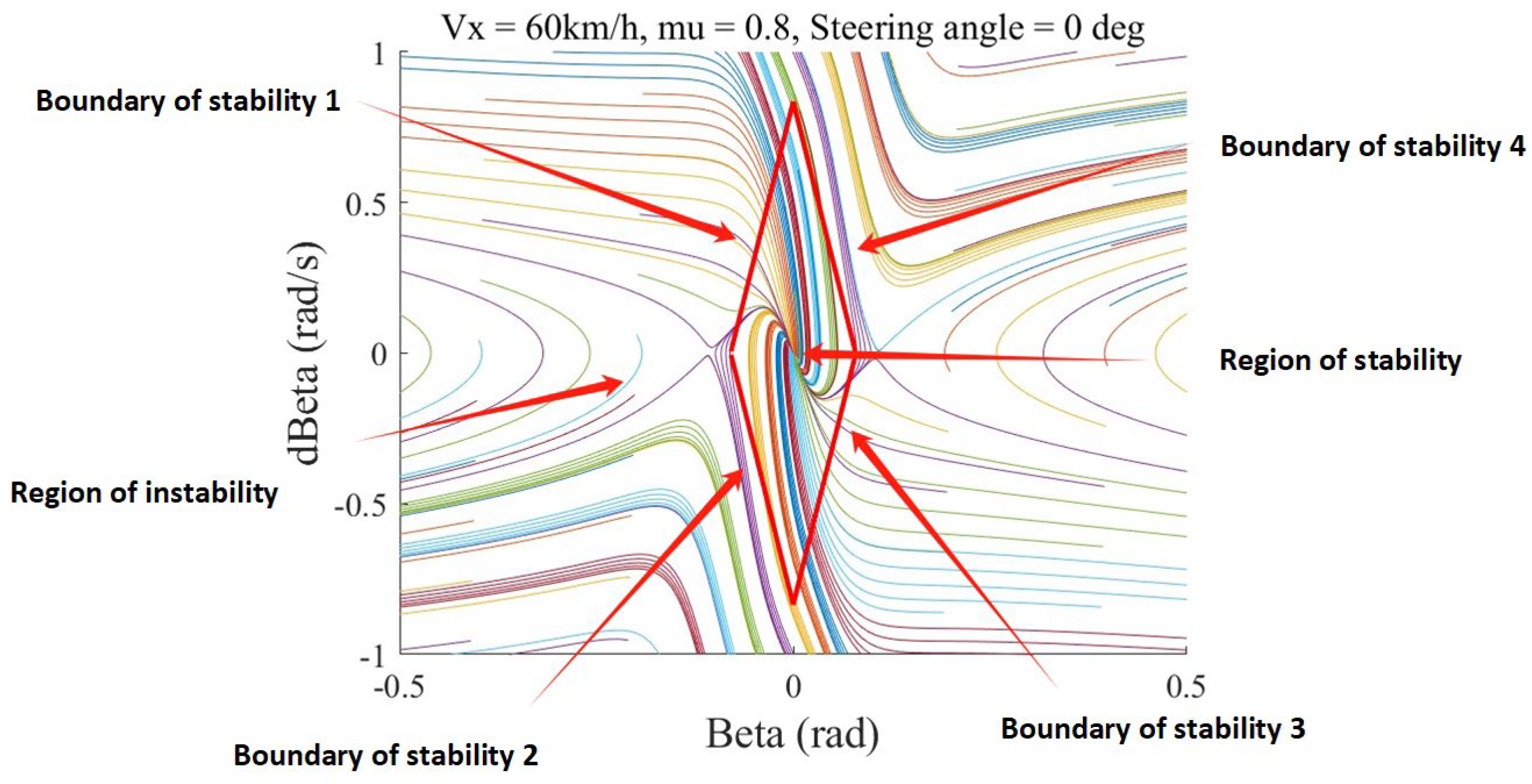
Under the given longitudinal velocity, the adhesion coefficient of the ground, and the front wheel angle, different initial values are assigned to Equation (32), the phase trajectory of the system is drawn, and the $\mathsf{\beta }-\dot{\mathsf{\beta }}$ phase plan is obtained.

Figure 5 shows the five-parameter diamond phase plan under the condition of ${\mathrm{v}}_{\mathrm{x}}$ = 60 km/h, μ = 0.8, and ${\mathsf{\delta }}_{\mathrm{f}}$ = 0. The five parameter values of the diamond region are the $\dot{\mathsf{\beta }}$ values of the upper and lower boundaries, the β values of the left and right boundaries, and the β value of the equilibrium point. We denote such by ${\dot{\mathsf{\beta }}}_{\mathrm{l}\mathrm{i}\mathrm{m}}^{+}$, ${\dot{\mathsf{\beta }}}_{\mathrm{l}\mathrm{i}\mathrm{m}}^{-}$, ${\mathsf{\beta }}_{\mathrm{l}\mathrm{i}\mathrm{m}}^{+}$, ${\mathsf{\beta }}_{\mathrm{l}\mathrm{i}\mathrm{m}}^{-}$, and ${\mathsf{\beta }}_{\mathrm{e}}$, respectively. The step size was selected under the given range of working conditions shown in

Table 2. Value ranges and step sizes of the three variables.

Variables	Range of Value	Step Size
$v_x$(km/h)	60~120	10
μ	0~1.0	0.1
${\delta }_f$ (°)	0~10	0.5

, and the simulation, as shown in Figure 5, was carried out in order to establish a relatively complete table look-up database of five parameter values. In addition, the boundary equations of the stable region under each working condition were obtained.

Table 3. Values of some database parameters.

${\mathit{v}}_{\mathit{x}}$ (km/h)	μ	${\mathit{\delta }}_{\mathit{f}}$ (°)	${\dot{\mathit{\beta }}}_{\mathit{l}\mathit{i}\mathit{m}}^{+}$	${\dot{\mathit{\beta }}}_{\mathit{l}\mathit{i}\mathit{m}}^{-}$	${\mathit{\beta }}_{\mathit{l}\mathit{i}\mathit{m}}^{+}$	${\mathit{\beta }}_{\mathit{l}\mathit{i}\mathit{m}}^{-}$	${\mathit{\beta }}_{\mathit{e}}$
60	0.8	0	0.835	−0.835	0.079	−0.079	0
60	0.3	0	0.265	−0.265	0.036	−0.036	0
80	0.8	0	0.672	−0.672	0.0685	−0.0685	0
80	0.3	0	0.303	−0.303	0.034	−0.034	0
120	0.8	0	0.48	−0.48	0.055	−0.055	0
120	0.3	0	0.104	−0.104	0.018	−0.018	0

shows some of the database parameter values obtained with the simulation.

In the $\mathsf{\beta }-\dot{\mathsf{\beta }}$ phase plan, the shortest distance between the vehicle state point in the stability domain and the boundary of the stability domain is defined as the stability degree. The degree of stability can characterize the degree of stability of the vehicle; moreover, the state points outside of the boundary of the stability domain are already in an unstable state, and their stability is 0. The calculation model of stability degree is as follows:

$$S_{\beta }=\left\{\begin{array}{l}0,B_i\le \stackrel{·}{\beta }+A_i\beta (i=1,2),B_i\ge \stackrel{·}{\beta }+A_i\beta (i=3,4)\\ \min \left[\left|\frac{\stackrel{·}{\beta }+A_i\beta -B_i}{\sqrt{{A_i}^2+1}}\right|\right](i=1,2,3,4),\\ B_i\ge \stackrel{·}{\beta }+A_i\beta (i=1,2),B_i\le \stackrel{·}{\beta }+A_i\beta (i=3,4)\end{array}\right.$$

(33)

where ${\mathrm{B}}_{\mathrm{i}}=\stackrel{•}{\mathsf{\beta }}{+\mathrm{A}}_{\mathrm{i}}\mathsf{\beta }(\mathrm{i}=1,2,3,4)$ are the four boundary equations of diamond shape; ${\mathrm{A}}_{\mathrm{i}}$ is the slope of the equation; and ${\mathrm{B}}_{\mathrm{i}}$ is the constant term of the equation.

According to the stability theory of the vehicle, the stability of the vehicle mainly depends on the yaw rate when the sideslip angle of the center of mass is negligible. Referring to the results found in the literature, the critical value of instability U for the yaw rate deviation is shown in

Table 4. Critical value of yaw rate deviation instability.

${\mathit{v}}_{\mathit{x}}$ (km/h)	U (rad/s)	${\mathit{v}}_{\mathit{x}}$ (km/h)	U (rad/s)
60	0.025	90	0.028
70	0.026	100	0.030
80	0.027	120	0.030

. According to the β-method theory, the yaw rate cannot effectively characterize the vehicle’s stability when the mass center lateral angle is large, and the influence of the mass center lateral angle on the vehicle’s stability is dominant. Therefore, the car’s instability judgment is carried out according to Figure 6.

In the stability control, the controller’s weight should be increased when the center of mass lateral deflection angle is large. The stability affected by the longitudinal velocity, the road adhesion coefficient, and the front wheel angle can effectively characterize this situation, as follows: near the diamond boundary, that is, when the stability is small, one situation is that the center of mass lateral deflection angle is large, then, the weight of the controller should be significant. The other case is that the centroid side angle is slight. However, in this case, the velocity of the centroid side angle is large, and the vehicle is about to enter the state with a large lateral angle of the center of mass, and so the weight of the centroid side angle controller should be significant now. Therefore, the stability degree can be used to reasonably allocate the controller weight P and be substituted into Equation (34) to obtain the weighted yaw moment ΔM, as follows:

$$\left\{\begin{array}{l}\Delta \mathrm{M}=\mathrm{P}\Delta {\mathrm{M}}_{\beta }+(1-P)\Delta {\mathrm{M}}_{\omega }\\ P=\frac{H}{H+S_{\beta }}\end{array}\right.$$

(34)

where H is the distance from the equilibrium point to the vehicle state point on the phase diagram.

3.4. Torque Distributor Design

The additional yaw moment obtained through the upper-level controller can be distributed to the four wheels to realize the control of the direct yaw moment. The vertical load of the wheel is related to the tire adhesion and the road adhesion coefficient. Assuming a constant value of the road adhesion coefficient, the adhesion force of the tire is proportional to the vertical load. Therefore, the side of the vehicle with a large axle load can output more longitudinal force, while the side with a small axle load will be relatively passive. The loads of the four tires are as follows:

$$\left\{\begin{array}{l}F{z}_{ff}=\frac{mgb}{2(a+b)}-\frac{m{a}_{x}h}{2(a+b)}-\frac{m{a}_{y}bh}{2B_f(a+b)}\\ F{z}_{fr}=\frac{mgb}{2(a+b)}-\frac{m{a}_{x}h}{2(a+b)}+\frac{m{a}_{y}bh}{2B_f(a+b)}\\ F{z}_{rf}=\frac{mga}{2(a+b)}+\frac{m{a}_{x}h}{2(a+b)}-\frac{m{a}_{y}ah}{2B_f(a+b)}\\ F{z}_{rr}=\frac{mga}{2(a+b)}+\frac{m{a}_{x}h}{2(a+b)}+\frac{m{a}_{y}ah}{2B_f(a+b)}\end{array}\right.$$

(35)

In order to improve the stability of the side of the wheel with a small axle load, the wheel torque can be distributed and controlled according to the ratio of the front and rear axle load, and the front and rear axle load can be obtained as follows:

$$\left\{\begin{array}{l}Fzf=G(\frac{b}{L}-\frac{a_{x}h}{L})\\ Fzr=G(\frac{a}{L}+\frac{a_{x}h}{L})\end{array}\right.$$

(36)

The torque distribution needs to meet the demand of the total driving force. The driving force between each wheel and the driving torque should meet the following relationship:

$$\left\{\begin{array}{l}\frac{(F{x}_{fl}+F{x}_{fr})}{Fzf}=\frac{(F{x}_{rl}+F{x}_{rr})}{Fzr}\\ \frac{B(F{x}_{fr}-F{x}_{fl})}{2Fzf}=\frac{B(F{x}_{rr}-F{x}_{rl})}{2Fzr}\\ T_{fl}+T_{fr}+T_{rl}+T_{rr}=F_{t_{d}des}*R\\ (F{x}_{fr}-F{x}_{fl})\frac{B}{2}+(F{x}_{rr}-F{x}_{rl})\frac{B}{2}=\Delta M^{*}\end{array}\right.$$

(37)

Since the moment of inertia of the wheel is small and the angular velocity of the wheel when the vehicle is stable is small, it can be regarded as zero. According to the dynamic equation ${\mathrm{I}}_{\mathrm{z}}\stackrel{•}{\mathsf{\omega }}=\mathrm{T}-\mathrm{RF}$, it can be solved as follows:

$$T_{ij}=R{F}_{ij}(ij=fl,fr,rl,rr)$$

(38)

Furthermore, the driving torque of each wheel can be solved as follows:

$$\left\{\begin{array}{l}{T}_{ff}=\frac{F{z}_{ff}}{(F{z}_{ff}+F{z}_{fr}+F{z}_{rf}+F{z}_{rr})}*(T-\frac{\Delta M*R}{2B_f})\\ T_{fr}=\frac{F{z}_{fr}}{(F{z}_{ff}+F{z}_{fr}+F{z}_{rf}+F{z}_{rr})}*(T+\frac{\Delta M*R}{2B_f})\\ T_{rf}=\frac{F{z}_{rf}}{(F{z}_{ff}+F{z}_{fr}+F{z}_{rf}+F{z}_{rr})}*(T-\frac{\Delta M*R}{2B_r})\\ T_{rr}=\frac{F{z}_{rr}}{(F{z}_{ff}+F{z}_{fr}+F{z}_{rf}+F{z}_{rr})}*(T+\frac{\Delta M*R}{2B_r})\end{array}\right.$$

(39)

In vehicle travel, the road environment is complex and changeable, and the road condition of the four wheels is not necessarily the same. Moreover, a single wheel, or part of the wheels, can still slip, so the four-wheel torque distribution scheme constructed above cannot guarantee that the vehicle can exert the maximum road adhesion ability in order to reduce as much as possible the risk of only a single wheel or part of the car wheel slipping. This subsection adds the drive anti-slip function to the wheel drive torque distribution scheme.

Drive anti-slip aims to reduce the slip of the wheel on the low-adhesion road surface, ensure the steering and relief ability of the vehicle, improve driving safety, reduce wheel wear, and improve wheel life. The slip rate of the wheel is calculated with Equation (40), as follows:

$${\lambda }_{\mathrm{i}}=\frac{{\omega }_{i}r-v_x}{{\omega }_i}\times 100\%$$

(40)

where ${\mathsf{\lambda }}_{\mathrm{i}}$ is the slip rate of the wheel, ${\mathsf{\omega }}_{\mathrm{i}}$ is the angular velocity of the wheel, r is the rolling radius of the wheel, and ${\mathrm{v}}_{\mathrm{x}}$ is the current longitudinal vehicle speed.

When slip occurs, the drive anti-slip function will adjust the wheel torque to control the slip rate of the wheel in the optimal slip rate range. This paper uses PI control to construct a driving anti-slip controller. The controller’s input is the deviation value between the expected and actual slip rates. In this paper, the expected slip rate is set to 15%, and the controller’s output is the wheel torque adjustment value.

$$\Delta T_i=K_p{e}_{\lambda i}+K_i{\displaystyle {\int }_0^t{e}_{\lambda i}}$$

(41)

The above design shows a drive anti-slip scheme for a single wheel, but for the whole vehicle if the torque of one side of the wheel is reduced. In contrast, if the torque of the other side is unchanged, an additional yaw moment will be generated so that the actual value of the additional yaw moment is not consistent with the value calculated by the yaw stability control algorithm, which will impact the vehicle’s yaw motion. Based on the above reasons, in order to ensure that the additional yawing moment value is not affected, the driving anti-skid function needs to add a multi-wheel coordination mechanism, that is, the left and right wheels need to reduce the same driving anti-skid adjustment torque value; however, if the left and right wheels are sliding, the reduced torque value will be too large, which will affect the vehicle dynamic performance. Therefore, based on balancing power and coordination, this paper takes the maximum value of the driving anti-slip adjusting torque of the left and right wheels as the common driving anti-slip adjusting torque.

$$\begin{array}{l}\Delta T_f=\max (\Delta T_{fl},\Delta T_{fr})\\ \Delta T_r=\max (\Delta T_{rl},\Delta T_{rr})\end{array}$$

(42)

Finally, the output of the torque value of each motor is as follows:

$$\left\{\begin{array}{l}{T}_{ff}=\frac{F{z}_{ff}}{(F{z}_{ff}+F{z}_{fr}+F{z}_{rf}+F{z}_{rr})}*(T-\frac{\Delta M*R}{2B_f})+\Delta T_f\\ T_{fr}=\frac{F{z}_{fr}}{(F{z}_{ff}+F{z}_{fr}+F{z}_{rf}+F{z}_{rr})}*(T+\frac{\Delta M*R}{2B_f})+\Delta T_f\\ T_{rf}=\frac{F{z}_{rf}}{(F{z}_{ff}+F{z}_{fr}+F{z}_{rf}+F{z}_{rr})}*(T-\frac{\Delta M*R}{2B_r})+\Delta T_r\\ T_{rr}=\frac{F{z}_{rr}}{(F{z}_{ff}+F{z}_{fr}+F{z}_{rf}+F{z}_{rr})}*(T+\frac{\Delta M*R}{2B_r})+\Delta T_r\end{array}\right.$$

(43)

In the above equation, $\mathrm{F}\mathrm{z}\mathrm{f}$ and $\mathrm{F}\mathrm{z}\mathrm{r}$ are the front and rear axle loads, respectively; h is the height of the centroid; ${\mathrm{a}}_{\mathrm{x}}$ and ${\mathrm{a}}_{\mathrm{y}}$ are the longitudinal acceleration and lateral acceleration, respectively; ${\mathrm{B}}_{\mathrm{f}}$ and ${\mathrm{B}}_{\mathrm{r}}$ are the front and rear wheel tracks; ${\mathrm{T}}_{\mathrm{i}\mathrm{j}}$ is the driving torque of the in-wheel motor; ΔT is the driving anti-slip adjustment torque of each wheel, where ff, fr, rf, and rr represent the left front wheel, right front wheel, left rear wheel, and right rear wheel, respectively; and R is the effective rolling radius of the wheel.

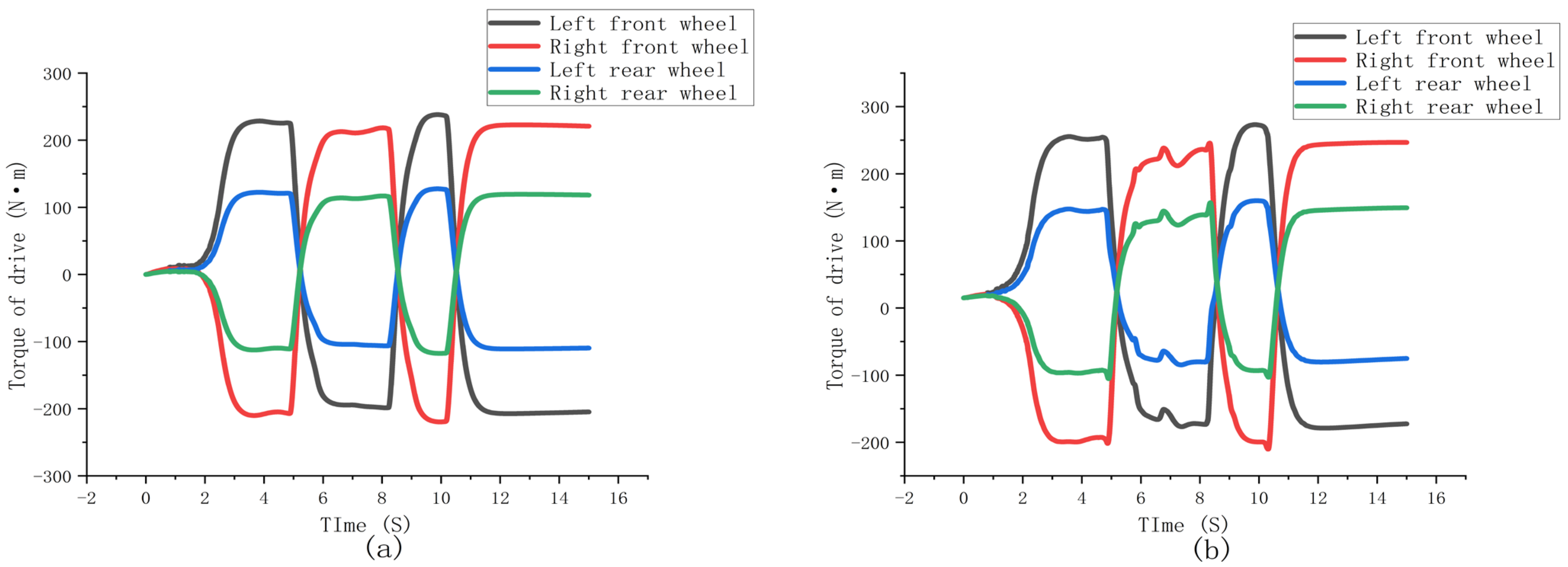
In order to verify the effectiveness of the anti-skid strategy proposed in this section, the driving torque of each wheel in the case of not considering anti-skid and considering anti-skid is calculated, respectively, on the double-moving line road with a road adhesion coefficient of 0.3 and a vehicle speed of 60 km/h, as shown in Figure 7. The driving torque of each wheel after considering anti-skid is lower than that without considering anti-skid. It can ensure that the vehicle has stability on the low-adhesion road surface, indicating that the designed torque distributor—considering the anti-skid strategy—is compelling.

4. Results

In order to verify the effectiveness and feasibility of the trajectory tracking strategy proposed in this study, the simulation is carried out on the Carsim–Simulink co-simulation platform. In this study, the double-shift line road, as well as Alt3 from FHWA, are used as the reference path, and the basic parameters of the vehicle are shown in

Table 5. Basic parameters of the vehicle.

Parameters	Unit	Value
Total vehicle mass $m$	$\mathrm{k}\mathrm{g}$	1413
Distance from the center of mass to the front axle $a$	$\mathrm{m}$	1.015
Distance from the center of mass to the rear axle $b$	$\mathrm{m}$	1.895
Moment of inertia of the vehicle at the z-axis $Iz$	$\mathrm{k}\mathrm{g}·{\mathrm{m}}^2$	1536.7
Front track width $B_f$	$\mathrm{m}$	1.675
Rear track width $B_r$	$\mathrm{m}$	1.675
Effective rolling radius of the tire $R$	$\mathrm{m}$	0.325
Height of the center of mass $h$	$\mathrm{m}$	0.54

.

In this paper, four groups of control tests are designed, as follows: the first group is the control system (control A), the second group is the MPC control system without particle swarm optimization (control B), the third group is the LQR control system (control C), and the fourth group is the SMC system control (control D).

4.1. Simulation Experiment of High-Speed Double-Moving Line Condition

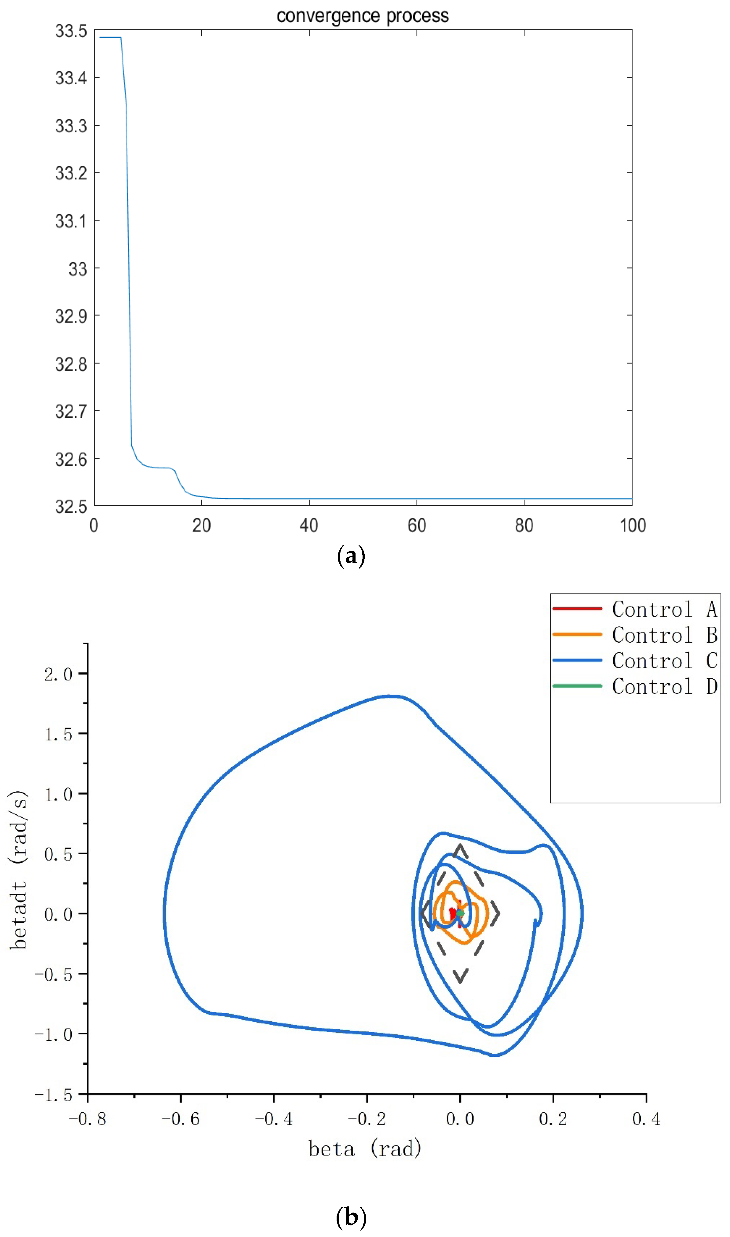
The high-speed double-line-moving condition can simulate the lane-changing action of the vehicle at high speed; moreover, the adhesion coefficient of the road is 0.8, and the speed is 120 km/h. The obtained simulation results are shown in Figure 8 and Figure 9.

According to Figure 8a, the PSO found the optimal ITAE value of 32.5 when approaching 20 iterations in this experiment. According to the phase trajectory diagram shown in Figure 8b, it can be seen that most of the phase trajectories of the control method using LQR are located in the unstable region. In contrast, the phase trajectories of the proposed control system, the MPC control system without PSO optimization, and the SMC control system are located in the stable region. Moreover, it can be seen that the phase trajectory of the MPC optimized by PSO is more concentrated than that of the unoptimized MPC, which indicates that the adaptive optimization of the MPC control parameters by PSO proposed in this paper is practical and improves the stability of the car.

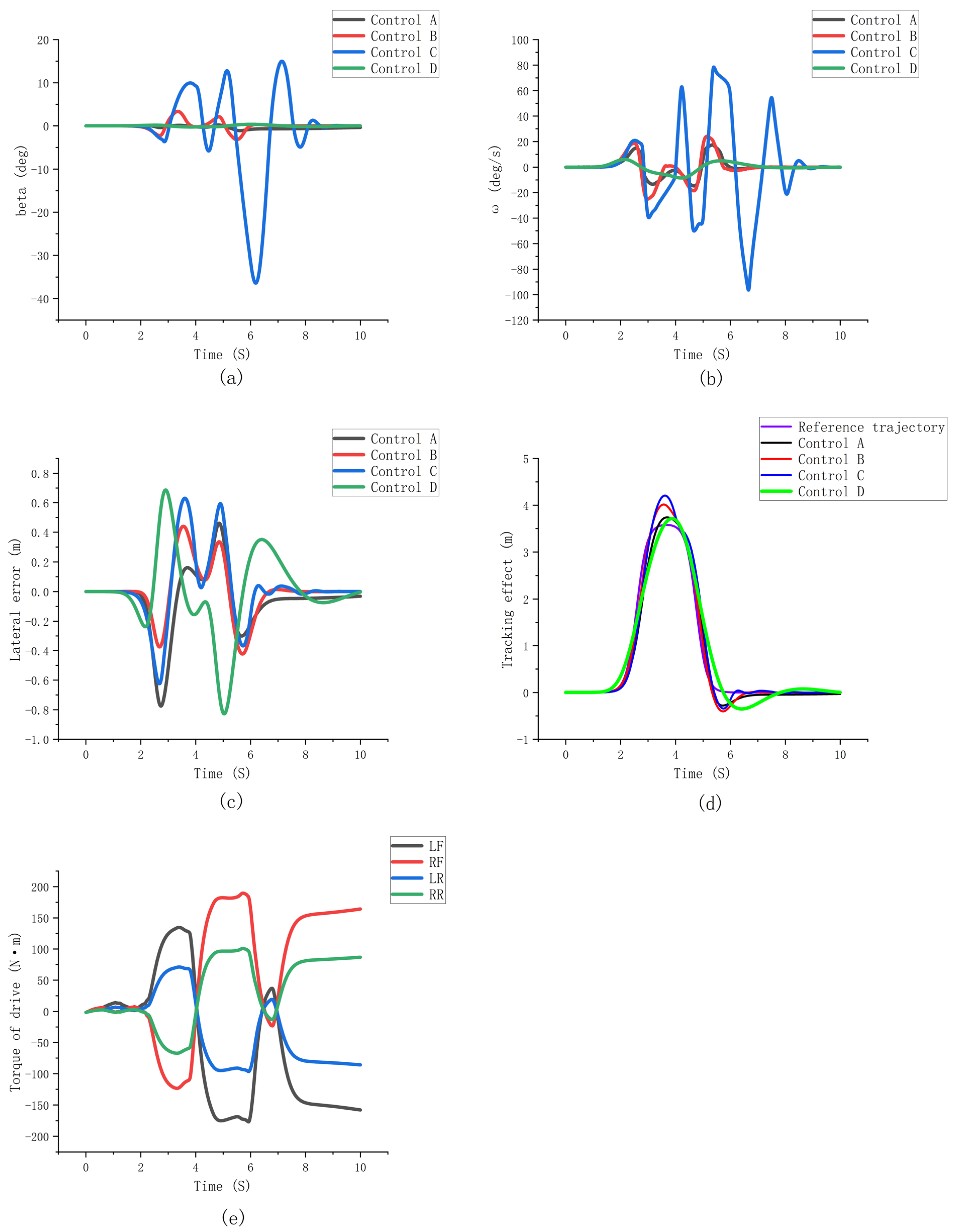
As shown in Figure 9a, the value of β of the proposed control system changes gently and tends to be 0, with an average value of 0.00632 deg and a peak value of 0.019656 deg, the minimum values of all of the control systems. The proposed control strategy shown in Figure 9b is evident compared to LQR and MPC optimization without PSO, but it is not as good as the SMC control system. Regarding the tracking accuracy, the average tracking error of the control system proposed in this paper is 0.13 m, which is significantly optimized compared to the SMC and LQR systems. However, the average value of the MPC control system without PSO is 0.103 m, which is slightly inferior. Figure 9e shows each in-wheel motor’s wheel driving torque output. The torque distributor distributes the driving and braking torque of the four wheels to make the vehicle achieve differential speed and better maintain body posture.

4.2. Simulation Experiment of Low-Attachment Double-Moving Line Condition

The low-adhesion double-line-moving condition can simulate the lane-changing action of the vehicle on rainy and snowy days. The adhesion coefficient of the road is 0.3, and the vehicle speed is 60 km/h. The obtained simulation results are shown in Figure 10 and Figure 11.

According to Figure 10a, the PSO found the optimal ITAE value of 33.5 when approaching 15 iterations in this experiment. According to the phase trajectory diagram shown in Figure 10b, it can be seen that the phase trajectories of the four control systems are located in the stable region. It can be seen that the phase trajectory of the MPC optimized by PSO is more concentrated than that of the MPC without optimization, which indicates that the control strategy proposed in this paper improves the stability.

As shown in Figure 11a, the value of β of the proposed control system changes gently and tends to be 0, with an average value of 0.00024 deg and a peak value of 0.002187 deg, the smallest value among all of the control systems. In Figure 11b, the control strategy proposed in this paper is significantly optimized compared to the other three control systems, with an average value of 0.054 deg/s, indicating that the proposed control system changes gently and increases the stability. Regarding the tracking accuracy, the average tracking error of the control system proposed in this paper is 0.055 m, which is significantly optimized compared to the SMC and LQR systems. However, the average value of the MPC control system without PSO is 0.053 m, which is slightly inferior.

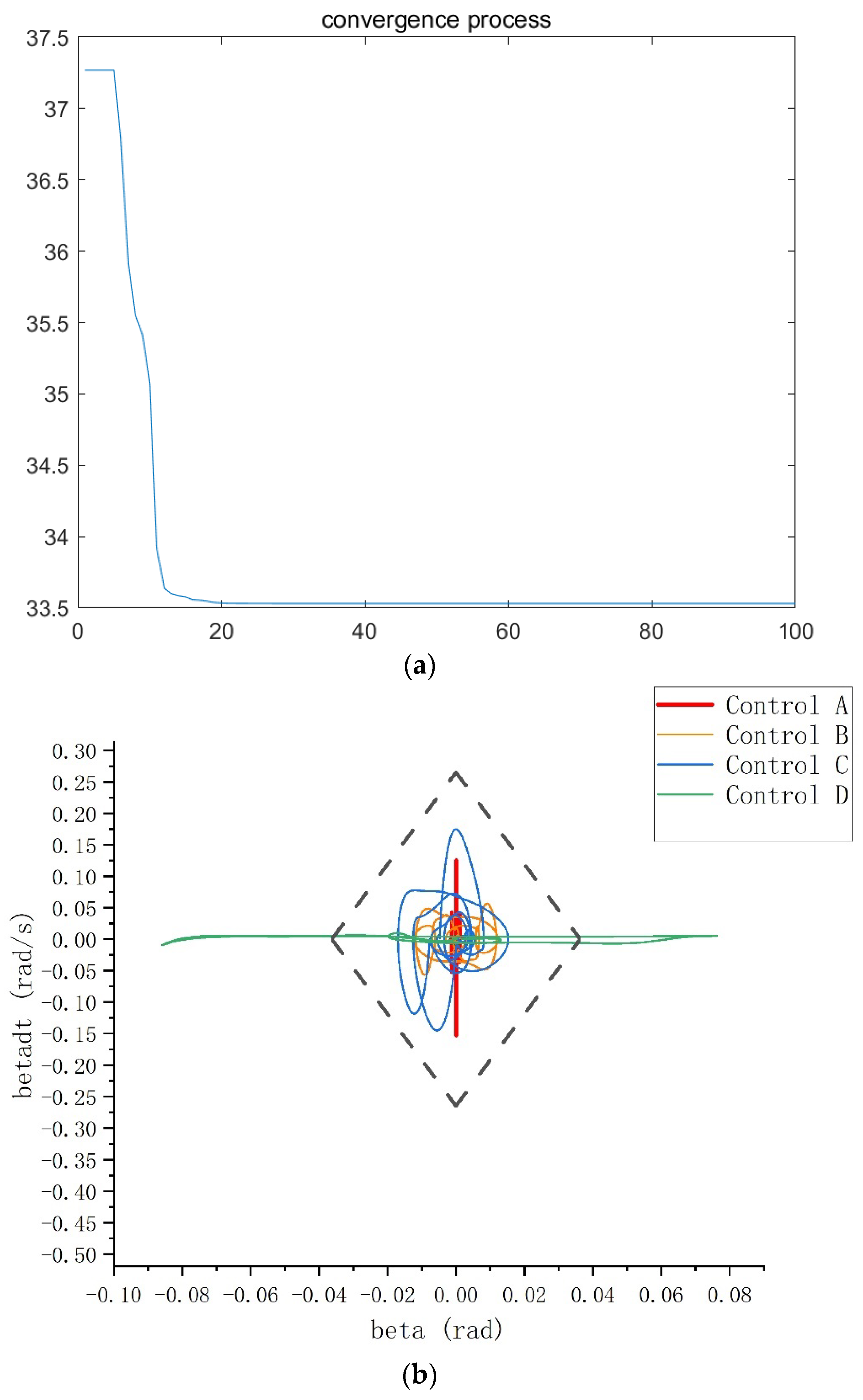
4.3. Simulation Experiments of Alt3 from FHWA Operating Conditions

In order to verify the adaptability of the control system designed in this paper to different roads, the Alt3 from FHWA is used as the reference path in this experiment. The road adhesion coefficient of the working condition is 0.8, and the vehicle speed is 60 km/h. The received simulation results are shown in Figure 12 and Figure 13.

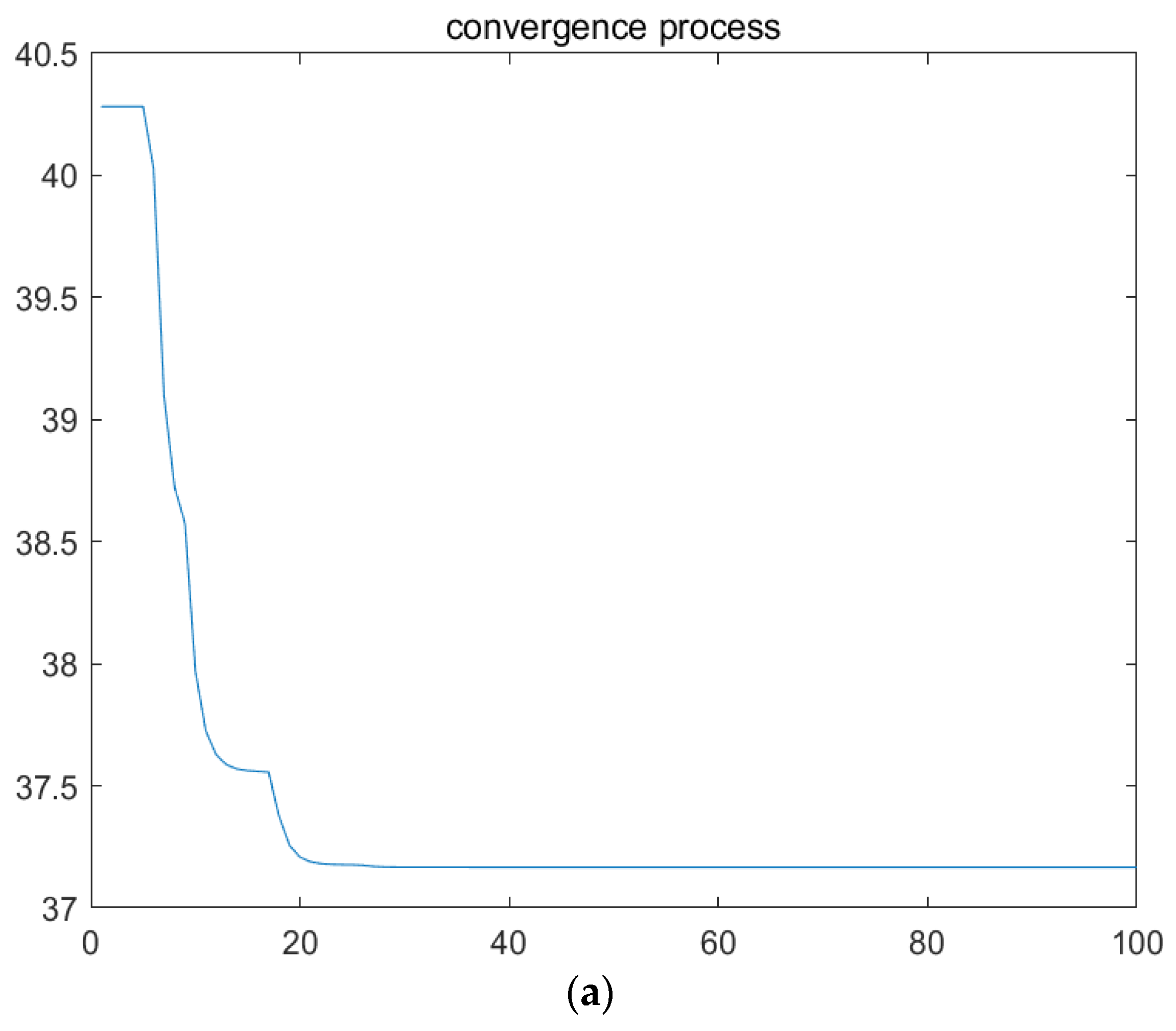
According to Figure 12a, the PSO found the optimal ITAE value of 37.25 when approaching 20 iterations in this experiment. According to the phase trajectory diagram shown in Figure 12b, it can be seen that the phase trajectories of the four control systems are located in the stable region, and it can be seen that the phase trajectory of the MPC optimized by PSO is more concentrated than that of the MPC without optimization. Therefore, the control strategy proposed in this paper improves the stability.

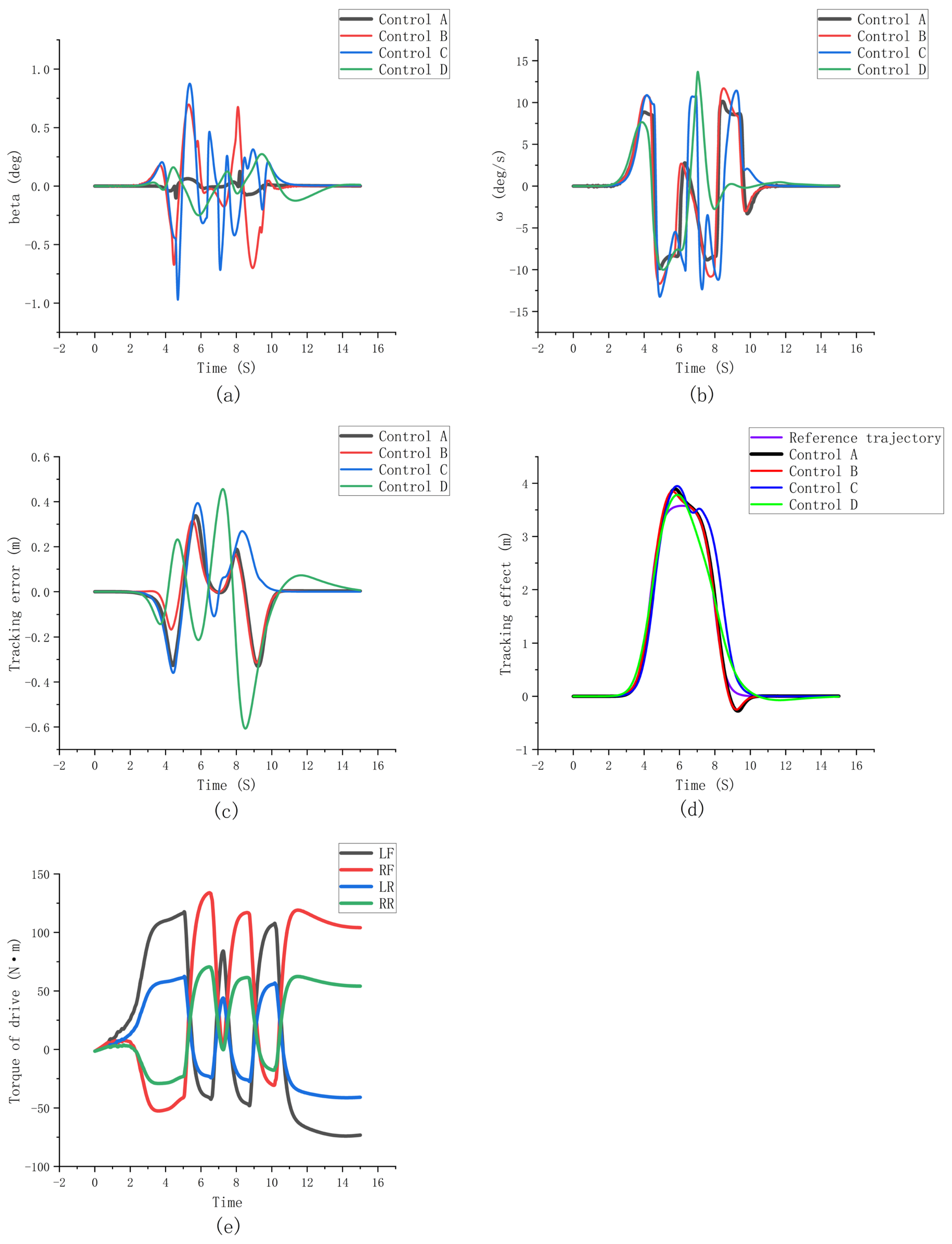
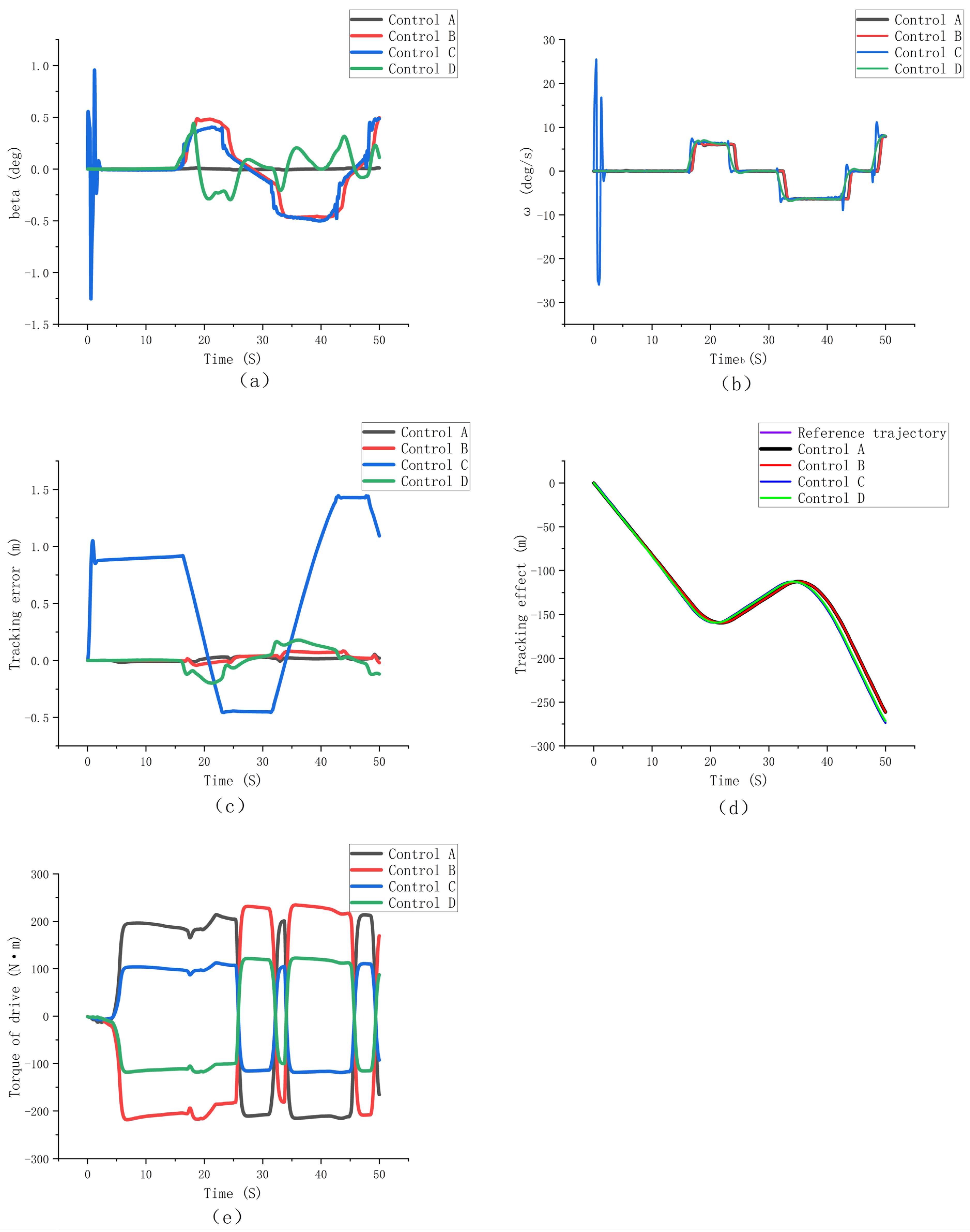
As shown in Figure 13a, the value of β of the proposed control system changes gently. It tends to be 0, with an average value of 0.00025 deg and a peak value of 0.01044 deg, which is the minimum value among all of the control systems, and the optimization effect is significant. In Figure 13b, the control strategy proposed in this paper has no noticeable difference compared to the other three control systems, and the average value is 0.234 deg/s. Regarding the tracking accuracy, the control system proposed in this paper is more accurate than the other three control systems, with an average value of 0.0015 m, which improves the accuracy of the trajectory tracking.

Based on the above experimental results and analysis, the yaw rate and yaw angle are essential indicators for evaluating the vehicle’s stability, representing the magnitude of the steering acceleration and the degree of body lateral deviation of the uncrewed vehicle when it moves laterally. The control system based on the PSO and phase diagram analysis designed in this paper effectively improves the accuracy and smoothness of the trajectory tracking while ensuring the vehicle’s stability under limited working conditions, such as high speed and low adhesion. In the experiment, the controller designed in this paper has the problem of degradation in trajectory tracking accuracy. After the analysis, the reason for this is that the stability and trajectory tracking control interact at high and low speeds. The improvement of stability will affect the change in trajectory tracking accuracy, and the change in trajectory tracking accuracy will also affect the improvement of the stability. Through the method of PSO and phase diagram analysis, this paper takes stability and tracking accuracy as the comprehensive optimization objectives and obtains the results of bi-objective coordination optimization.

5. Conclusions

Aiming to solve the trajectory tracking problem of distributed driving vehicles under extreme conditions, such as high speed and low adhesion, this paper designs a trajectory tracking control system to ensure the vehicle’s stability, improve the trajectory tracking accuracy, and realize the coordinated optimization of dual control objectives. The simulation experiments of related working conditions are carried out using Carsim–Simulink co-simulation. The results show that the coordinated control strategy proposed in this paper can simultaneously ensure trajectory tracking accuracy and improve the vehicle’s driving stability under the limited working conditions of high speed and low adhesion. However, the particle swarm optimization algorithm designed in this paper only optimizes the two weight coefficients Q and R in real time. It does not consider the influence of the control and prediction time domains on the control effect. In addition, the working conditions selected in this experiment are established scenarios, while actual road conditions are changeable. Therefore, future research can introduce a state parameter estimator that combines visual images with dynamic information to achieve adaptive stable tracking control for different road conditions and explore new PSO algorithms to control the control and prediction time domains. In addition, this study has only stayed in the simulation stage without actual testing, and the combination of different control strategies has certain complexity, which may bring challenges to the actual application and calibration.