Featured Application
The outcome of this study has the potential to open a new direction to optimise the success of asset management and of financial markets in general. The new focus is not algorithms, but the non-conscious mind in humans.
Abstract
In the world of finance, considerable attention is given to improving machine learning techniques to predict the future of stock markets. However, for obvious reasons, this turns out to be an unsolvable mission, most likely because the real world is not driven by algorithms but by human beings. In response to this, the present study has its focus on raw affective responses in actual asset managers during their decision making regarding controlled financial scenarios. Nineteen asset managers were invited and asked to make sell/buy decisions related to visual presentations of three different price developments of different assets. The three scenarios were “crash”, “stable” and “gain”. Parallel to their decision making, startle reflex modulation (SRM) was used to measure non-conscious affective responses without demanding any respective explicit responses (no conscious language processing involved). Interestingly, two further factors were introduced. First, all participants had to make their decisions once while being informed that 0% prior investments (low exposure) have been made into the presented assets, and once being informed that a large investment consisting of 25% of ones’ overall portfolio has been made prior to making the decision (high exposure). Second, the factor experience was included dividing all participants into two groups, one with low experience and the other with high experience. First, across both these extra factors, it was found that “crash” scenarios resulted in the most negative affective responses. The most positive affective responses were found for “gain” scenarios, while the “stable” condition was in between. Interestingly, the factor of prior investment (i.e., exposure) had an effect. Non-conscious affective responses during decision making related to the “stable” condition varied as a function of “exposure”. In the low exposure condition, affective responses to decision making during the “stable” scenario were most negative, even more negative than in “crash” scenarios. The factor experience also had an effect, but due to the small sample size, no significant interaction occurred. However, t-tests revealed the same significant effects in the experienced group as found in the 0% prior investment condition. To our knowledge, this is the first empirical investigation measuring non-conscious affective responses during decision making in the context of asset management. Thus, this study might form an interesting basis for new strategies to explore non-conscious human brain functions instead of inventing new algorithms to make asset management more successful.
1. Introduction
Some of us are quite interested in increasing their wealth by trading various kinds of assets on the finance market. So, not surprisingly, forecasting financial markets is a highly desired goal for all investors, but respective prediction is a challenge. Some do it by themselves after self-education, while others consult professional asset managers that create portfolios for their clients. An asset manager looks after a portfolio and makes changes to it; in other words, they maintain and trade acquired investments. Obviously, while trying to maximise the value of an investment portfolio, one needs to make decisions, some of which follow a riskier approach, while others are made on a rather conservative basis. Risk aversion versus a more adventurous style is more or less the basic framework within which decisions are made [1]. In contrast to humans like asset managers or private people making trading decisions, these decisions can also be made by software algorithms trained to maximise profit. Since the advent of information technology (IT), there has been a strong trend in optimising such algorithms [2], and the rise of ever-more efficient algorithms in the frame of machine learning technology seems to promise secure financial profits [3,4], even though this is actually impossible. In our opinion, the critical point is that this IT strategy neglects the fact that the finance market itself is not a result of machines, but of human beings. If the world of economy was driven by sole digital decision making, it would indeed most likely be possible to derive secure profit from pure calculations. However, it is humans, more precisely human brains, that drive financial markets, and human brains are far from being simple cognitive and rational processing machines. Humans in high positions like Chief Executive Officers (CEO) influence the value of assets, and their decisions are not purely rational. They negotiate, they plan, they have visions, and all of that is a result of cognitive and affective processing in their brains.
At this point, it seems useful to build up a good meta-perspective on humans (especially their brains) as organisms resulting from a long evolutionary process. From a neurobiological perspective, the function of the human brain is to produce adapted behaviour [5]. Thereby, behaviour means any bodily movement resulting from the contraction of at least one muscle [6]. Behavioural adaptation happens via information processing performed by neural networks, and information means anything that enters the brain via sensory systems (including sensory systems for external as well as internal stimuli) or that can be retrieved from the multiple memory systems [7]. In the end, the brain is largely a processing organ that adapts (modifies) behavioural output in a constantly changing world inside and outside the body. Adaptation can be understood as continuous decision making, which happens consciously from a subjective perspective, but from the brain’s perspective even more non-consciously. It has been emphasised in the past that the attempt to verbalise especially affective content can suffer from a phenomenon called cognitive pollution [8]. Furthermore, an eye-opening fact is that there is no picture and no tone in the brain. All that is in the brain is physiological phenomena (ions flowing through cellular membranes of neurons and other cells) [9]. Very important for the current context of conscious decision making related to stock market scenarios is that information that is processed by the brain has cognitive (what is something?) and affective (how is something?) aspects. Although the brain uses both qualities to make decisions, these are initially processed by separate neural networks. These two networks are communicating with each other, but they are still separate systems, the affective system being older (in evolutionary terms) than the cognitive system [6].
Cognitive processing can be understood as analogous to rational processing, which refers to the idea of humans being so-called “homines oeconomici” [10]. Irrational processing, on the other hand, which is often defined as emotional processing, is connected to affective processing. At this point, it is not important to define “emotional processing” separately, but from a neurobiological perspective, it seems more appropriate to use the term “affective processing” as defined above [5]. More recent literature highlights the idea that the term “homo oeconomicus” should perhaps be replaced by “homo emoticus” [11] or even better “homo affecticus”, see [5]. It is affective processing that guides human behaviour more dominantly on a very basic level, and it influences pure rational decision making, turning it into something that again most people would call emotional decision making. A widely known game, the so-called ultimatum bargaining game, demonstrates very clearly that human brains surely are not solely driven by rational decisions [12]. In that game, one player proposes a certain split of available money (e.g., keeping eight and offering two coins), while the other player has the power to accept or reject the respective offer. In case of acceptance, both players get their share, but in case of rejection, no player gets anything. Pure rational calculation would mean accepting every offer, even only one coin, but the reality shows that, due to feelings of unfairness, such offers are rejected. The social unfairness aspect becomes even clearer when such offers are not made by a human, but by a computer. Then, there is less unfairness felt, and more “unfair” offers are accepted. The take-home message is clear: human brains take affective processing into account even when it comes to financial decisions. Thus, to investigate financial decision making, it is more helpful to collect affective data instead of purely focusing on cognitive data. The most widely chosen strategy to investigate decision making is asking questions that require explicit responses. Crucially, this approach is potentially misleading, largely because of implicit processing taking place [13]. Implicit processing refers to retrieved information feeding into decision making in the absence of any awareness of the information itself [14]. Surveys and pure observations cannot gain access to such information processing; only objective methods are capable of doing so. Since affective processing is older than cognitive processing, it is also more difficult to verbalise respective content, because language is a rather young function in terms of evolution [5,6]. It has been shown that implicit word processing can be objectively measured via electroencephalography (EEG) [13,15], but EEG is mainly sensitive to cortical processing in the brain, while affective processing primarily happens subcortically. For this purpose, startle reflex modulation (SRM) is an adequate tool; see, e.g., [16]. The very simple underlying phenomenon is that one is more startled by a constant startle probe while being exposed to negative content compared to positive content. In other words, a startle response is enhanced during negative stimulus exposure, and it is reduced during positive stimulus exposure. Hence, the method is called startle reflex modulation.
Among a few others [17,18], SRM is mainly sensitive to valence-related aspects of a stimulus, and it does not require any explicit responses; see, e.g., [19]. In other words, there is no need to ask any questions while conducting an SRM experiment. It has been widely used for various applied questions of interest. Possible applications are more or less unlimited. In the past, controlled acoustic [20], visual [21], olfactory [22] and even taste stimuli [23] have been delivered within SRM experiments to measure affective responses to them. The most crucial point is that no verbal responses need to be recorded. This is of particular interest, because self-reported responses to particularly affective content can be “cognitively polluted”, as has already been pointed out [8]. Just to mention a few more details, one study investigated affective responses in ecologically valid environments such as driving through a virtual tunnel [24], while affective responses during virtual walks (via Google Street View) through districts in Paris with different median real estate prices were measured in another study [19]. A significant reduction in startle responses during pleasant film clips and significant augmentation during unpleasant film clips were found [25]. Fear-relevant, unpleasant, but fear-unrelated, neutral and pleasant scenes were presented to fearful participants, who showed potentiated startle responses during exposure to pictures of fearful objects [26]. This phenomenon was independent of respective autonomic responses. Even when study participants were asked to imagine the content of a prior learned fearful sentence, their startle responses were enhanced, and their cardiac rates were faster compared to imagery of neutral sentences [27]. While psychopaths showed similar autonomic and self-report responses to unpleasant stimuli depicting mutilations, aimed guns and snakes, among others, there eye blink responses did not follow the expected pattern. Psychopaths showed significant reductions in eye blink responses to unpleasant stimuli [28]. Overall, SRM turned out to be highly sensitive to raw affective responses originating from structures in the limbic system.
For the purpose of the present study, it has been decided to apply SRM in order to measure non-conscious affective responses in asset managers while making buy or sell decisions in different scenarios of various underlying assets to different value development scenarios. The aim was to contribute to a better understanding of brain processes underlying the respective decision making and to discuss a possible role of SRM in this context. This study is of an exploratory nature. It is meant to focus more on the human side of asset management rather than algorithms that are created for better price development predictions. Finally, one could link this studies’ approach to so-called talent management (TM) [29] with a focus on neuroscience instead of programming. The use of knowledge and expertise from neuroscience is more and more highlighted as an attractive and beneficial strategy [30].
2. Materials and Methods
2.1. Participants
A total of 19 active asset managers (14 men) were invited to participate in this study. Their mean age was 35.4 (SD = 8.3) years, and they had a mean number of 10.1 (SD = 7.8) years of experience regarding asset management. They all had normal or corrected to normal vision and no hearing problems. They all signed a consent form and were told that they could terminate their participation in the experiment anytime without any consequences.
2.2. Stimuli
Images of actual asset price developments (from July 2018 to March 2020) were visually presented for 6 s. They showed the actual historical development of one asset including several corresponding value indicators (see descriptions below) until March 2020 followed by a simulation of one of three possible scenarios (until March 2022). The three scenarios were “gain”, “stable” and “crash” (see Figure 1). Those recent development aspects formed the varied basis for decision making regarding selling or buying. In addition, the corresponding value indicators (bar plots on the right side of all scenarios) were meant to provide a comprehensive understanding of recent price and valuation dynamics of an underlying asset, such as the NIKKEI-Index, to an informed observer on the basis of longer-term information. In order to contextualise the price development in the line chart effectively, the visual representation employs bar plots on the right side to depict the historical range of pertinent variables (e.g., Price, CAPE, REER) over the preceding decade. Additionally, it incorporates graphical elements such as the geometric mean (illustrated by an orange line) and the most recent observed price (depicted as a light blue point) within the specified time period. Visualizations of this or similar nature are extensively used within the financial industry to furnish contextualization for price movements, underscoring their utility and relevance in facilitating informed decision-making processes. CAPE (Cyclically Adjusted Price Earnings Ratio) is a valuation measure that uses real earnings per share over a 10-year period to smooth out fluctuations in corporate profits due to the business cycle. It provides a more stable view of a company’s or market’s earnings relative to its price, offering insights into whether a particular asset is overvalued or undervalued compared to historical norms. REER (Real Effective Exchange Rate) is a measure of a country’s currency in relation to the currencies of its trading partners, adjusted for inflation. It provides a broader understanding of a currency’s value by considering not only its nominal exchange rate, but also the relative price levels between countries. REER helps financial professionals to assess whether a currency is overvalued or undervalued. All participants were familiar with those indicators (see Figure 2) and were instructed to mainly focus on the recent scenario regarding the actual curve display as well as on those further indicators on the right of each image presentation.
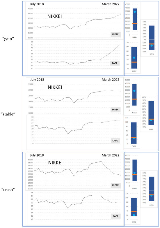
Figure 1.
Example stimuli: variations in one asset (NIKKEI stock market index) showing what the three different development scenarios (“gain”, “stable” and “crash”) look like. On the right, some indicators are included. Please, see Figure 2 and respective explanations in Section 2.2 Stimuli.
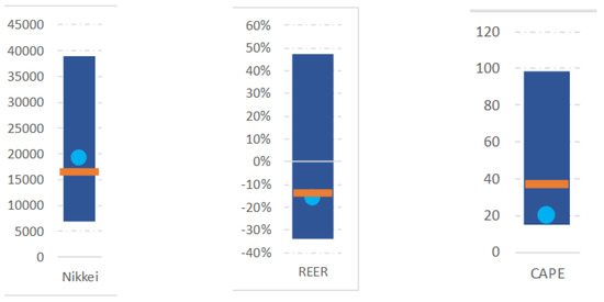
Figure 2.
Example indicators presented on the right side of all scenario presentations. Please see respective explanations in Section 2.2 Stimuli.
2.3. Procedure
All participants were invited to volunteer in the current study. After giving their full consent to take part in the experiment, they were seated on a comfortable chair and the respective sensors were attached. In front of them on a table was a monitor via which all images were presented. The instruction was to think about a sell or buy decision for every single value development scenario during its 6 s long appearance and to share the respective decision outcome through clicking on one of two available buttons on the screen using a computer mouse. Decision making was supported by adding various details to each stimulus presentation. Besides the actual development of the respective value, there were three further details displayed as bar plots (see Figure 2).
Twenty variations (different assets like stock indices, currencies and commodities) of each scenario were used summing up to a total of 60 images (3 × 20) on the basis of which participants had to make sell/buy decisions. Crucially, three of the twenty variations in each category had an associated startle probe occurring between seconds 5 and 6. For more information about startle reflex modulation, see point 2.4. Each 6 s-long displayed image was followed by a 1 s black screen and then a response screen appeared with the two decision buttons (buy/sell). Participants had up to 3 s to respond. Whenever they responded, a 1 s black screen followed by a 1 s white fixation cross (on black background) and a further 1 s black screen were presented before the next image appeared. Figure 3 shows a visualisation of this experimental design.
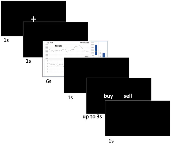
Figure 3.
Visualisation of the experimental design. Each image, which required decision making regarding selling or buying, was presented for 6 s followed by a black screen shown for 1 s. Then, a black response screen followed with the options “sell” or “buy” to click on for a maximum of 3 s (the experiment continued whenever a response was given or after the 3 s). Finally, a black screen was presented for 1 s followed by a black screen with a white plus shown for 1 s (i.e., fixation point) and then a further black screen for 1 s until the next actual stimulus image was displayed.
2.4. Startle Reflex Modulation
Eye blink responses to 50 ms short acoustic white noise probes (105 dB; delivered via headphones fully covering both ears) were recorded with bipolar electromyography (EMG). To achieve the respective sound pressure level, a commercial headphone pre-amplifier was used (Behringer, Willich, Germany; MicroAMP HA400). EMG was carried out with a Nexus-10 mobile recording system (i.e., a 10-channel system) (Mind Media BV). Muscle potential changes in the musculus orbicularis oculi of the left eye were measured in each participant and stored on a laptop computer. Dual-channel electrode cables with carbon-coating and active shielding technology for low noise were used with an additional ground electrode, which was placed on the right cheek. The EMG sampling rate was in fact 2048 per s, but a band pass filter from 20 to 500 Hz was applied during online recording, which is a standard procedure to include only muscle-related signals. Raw EMG data, which mainly carry frequency signals, were then recalculated into amplitudes using the root mean square (RMS) method. For this purpose, an inbuilt calculation option from the software package Biotrace+ from Mind Media (BT-NX10B-EN; 2018A1) was used; see [31]. The software package Biotrace+ (run on a laptop computer) was used for data collection, data pre-processing as well as running the experiment.
2.5. Data Analysis
All amplitude values were finally entered into an SPSS (version 27) matrix for descriptive and analytical statistics. In order to test main factor and factor interaction effects, an ANOVA (Analysis of Variance) was calculated (Greenhouse–Geisser corrected values are reported) followed by t-tests to identify the possible differences between separate mean values of single conditions. The Bonferroni–Holm correction was applied. For t-tests with the largest mean differences, the adjusted α is 0.017; for the second largest mean differences, it is 0.025; and for the third largest mean differences, it is 0.05.
3. Results
3.1. Overall Scenario Effect
The strongest eye blink responses resulted from decision making during exposures to “crash” scenarios, followed by “stable” and finally by “gain” scenarios. For descriptive statistics, see Table 1 and Figure 4. An analysis of variance (ANOVA) resulted in a significant main scenario effect (F(2,18) = 3.347, p = 0.037; η² = 0.034) (Greenhouse–Geisser corrected). Posthoc t-tests (Bonferroni–Holm corrected) revealed a significant difference between the “gain” and “crash” scenarios (p < 0.001; survives adjusted α of 0.017) as well as between the “gain” and “stable” scenarios (p = 0.021; survives adjusted α of 0.025). The difference between the “crash” and “stable” scenarios is not significant (see Table 2).

Table 1.
Mean eye blink responses (including standard deviations) for all three scenarios (“gain”, “crash” and “stable”). Note that the “crash” scenario is associated with the strongest eye blink responses, which translates to the most negative non-conscious affective processing during decision making in this case.
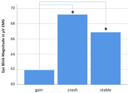
Figure 4.
Bar diagram showing mean eye blink responses related to all three scenarios (“gain”, “crash” and “stable”). Note that the “crash” scenario is associated with the strongest eye blink responses, which is interpreted as the most negative non-conscious affective responses for this scenario. Asterisks mark significant t-test results.
Table 2.
t-test results: mean eye blink responses compared for each possible pair of conditions. Note that the comparisons between “gain” and “crash” as well as between “gain” and “stable” resulted in significant differences between those pairs (surviving Bonferroni–Holm correction for multiple comparisons), while the conditions “crash” and “stable” did not elicit significantly different eye blink responses.
3.2. Scenario Effects Depending on High Exposure (25%) versus No Exposure (0%)
Descriptive statistics results in the interesting finding that the pattern of the above-described scenario differences regarding eye blink responses can be seen very clearly in the 25% exposure condition, but not in the 0% exposure condition (see Table 3 and Figure 5). In the 0% exposure condition, the “stable” scenario elicited the strongest eye blink responses instead of the “crash” scenario. Unfortunately, the interaction of the above-mentioned scenario effect with the factor “exposure” showed only a weak trend but turned out not to be significant (p = 0.165; F = 1.857). The lack of significance is most likely due to a relatively low number of participants (who were not easy to recruit), which is one of the limitations in this study. Nevertheless, t-tests were still calculated to compare each possible pair of scenarios for each exposure condition separately (see Table 4). In the “25% exposure” condition, the results resemble the ones found across both exposure conditions (see Table 1 and Figure 4). The “crash” scenario elicited the strongest eye blink responses (significantly different to the “gain” scenario), while the “stable” scenario falls in between the “gain” and “crash” scenarios (see Figure 5). Surprisingly, however, in the 0% exposure condition, the “stable” scenario elicited eye blink responses similar to the “crash” scenario (even stronger) (see Figure 5). It is thus interpreted that the “stable” scenario elicited the most negative (aversive) affective responses during decision making regarding buy or sell in the 0% exposure condition, which is different to the 25% exposure condition, in which the “crash” scenario elicited the most negative (aversive) responses (as found by not taking the “exposure” factor into account).
Table 3.
Mean eye blink responses (including standard deviations) for all three independent variables (the scenarios “gain”, “crash” and “stable”) for both exposure conditions separately. Note that in the no exposure condition the “stable” scenario elicited the strongest mean eye blink response, which translates to most negative non-conscious affective processing during decision making in this condition.
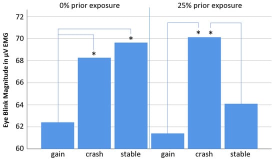
Figure 5.
Bar diagram showing mean eye blink responses related to all three scenarios (“gain”, “crash” and “stable”) for each exposure condition separately. Note that the “crash” scenario is associated with strongest eye blink responses only in the 25% exposure condition, while the strongest eye blink responses in the 0% exposure condition were elicited by the “stable” scenario, which is interpreted as most negative non-conscious affective responses associated for this scenario in the 0% exposure condition. The asterisks mark significant Test results.
Table 4.
t-test results for comparisons between all possible scenario conditions for 0% and for 25% exposure separately.
3.3. Scenario Effects Depending on Experience
Descriptive statistics show that the overall found scenario effect only occurred in case of no experience (Figure 6 and Table 5). Unfortunately, neither the factor experience itself nor the interaction between scenario conditions and experience turned out to be significant, which is mainly due to small sample sizes. However, due to the explorative character of this study, we decided to present those results and ran further t-test calculations comparing each scenario pair with each other for each experience condition separately (see Table 6).
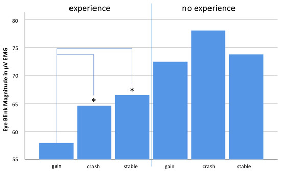
Figure 6.
Bar diagram showing mean eye blink responses related to all three scenarios (“gain”, “crash” and “stable”) for each the experienced and the no experienced group separately. Note that the overall scenario effect described in Section 3.1. (see Figure 4) can only be seen in the no experience group. In the experienced group, the pattern of results resembles the one seen in the 0% prior exposure condition (see Figure 5). In the experienced group, it is the “stable” scenario that elicited the strongest eye blink response, which is interpreted as the most negative non-conscious affective responses associated for this scenario in this group. Asterisks mark significant Test results.
Table 5.
Mean values of all possible scenario conditions for the high experience and the low experience group separately.
Table 6.
t-test results for comparisons between all possible scenario conditions for experienced and for un-experienced participants separately.
4. Discussion
The present exploratory study was designed to contribute to a better understanding of financial decision making in humans in the context of asset management by introducing an objective method to this field. Startle reflex modulation (SRM) was applied to describe non-conscious affective processing in asset managers during their sell/buy decisions related to varying developments of different asset prices. While being more explorative than hypothesis-driven, the value of this study lies in the focus on non-conscious affective processing, which is not accessible through survey-based investigations, and SRM has long been proven to be a highly reliable tool [32]. The advantage of measuring non-conscious information processing is that it provides insight into the human mind that not even the same mind itself can get through conscious deliberation. In this regard, a recent review on SRM studies focusing on psychopathologies showed that depressed brains process positive emotion pictures significantly more negative (subcortically) compared to healthy brains in the absence of this negativity being mirrored in respective explicit responses [33]. In addition, psychopaths show significantly reduced startle responses when viewing graphic images, while their explicit responses mirror similar negativity levels compared to healthy controls [28]. Both outcomes demonstrate that SRM seems to indeed allow access to otherwise hidden information processing in the human brain, which, as mentioned in the introduction, has a dominant influence on decision making. SRM has been known to work in humans since the 1980s [34,35], when facial expressions were presented to participants, while they were startled with loud white acoustic noise. The pattern of results (respective eye blink responses) clearly showed that positive stimuli like smiling faces reduce the startle response to a constant startle probe, while a negative stimulus enhances it. If a stimulus has a controlled affective aspect, those results are very robust and have been replicated and confirmed numerous times, even for pleasant and unpleasant music as stimuli [20]. On the other hand, SRM is able to efficiently measure affective aspects of any stimuli without requiring explicit responses, which, due to conscious deliberation, might pollute raw affective information when put into words, a concept called cognitive pollution of raw affection, as already mentioned above [8]. In that sense, a number of applied studies have shown that SRM is indeed a useful tool to define non-conscious affective responses to more or less all kinds of stimuli (see Introduction). SRM has even been introduced to the world of marketing and Neuro Information Systems [36].
SRM studies in the context of financial decision making are rare; in fact, the use of objective methods in general is rather limited. In one of very few cases, authors of a recent SRM study on reward-related motivational aspects during feedback interpret their results in terms of startle potentiation when missing out on a reward rather than in terms of inhibition as a result of winning [37]. In other words, they favour the idea that motivational tendencies during reward feedback are mainly reflecting aversion related to reward omission rather than appetitive responses in case of a gain. In their experiment, the largest startle reflex potentiation occurred in cases of the largest reward omission. These results are interesting in the context of the so-called prospect theory; see [1]. However, it should be emphasised that the largest possible amount to win was only USD 0.20. Nevertheless, while the nature of this experiment is fundamentally different to the one in our study, because their study did not include any decision making, it is nevertheless worthwhile to follow the idea that aversion plays a more crucial role than positive aspects of a stimulus, maybe in particular when stimuli are of monetary nature. However, similar results were found for facial expressions as stimuli. However, knowing that facial expression stimuli are usually fake (pictures were taken in the absence of true respective feelings behind the faces), these results have to be treated with great caution [21].
In the present study, no baseline responses were collected, and it is thus not possible to infer any absolute points on the appetitive/aversive continuum. However, the relative response differences between the scenarios “gain”, “stable” and “crash” show a clear pattern and, crucially, manipulations of eye blink responses collected in the present study indeed reflect affection during financial decision making related to varying scenarios of asset price developments. Participants had to decide whether to buy or sell distinct assets for all three scenarios. Leaving out the “exposure” factor (i.e., percent prior investment), the smallest mean startle response occurred for “gain” scenarios that were mostly associated with sell decisions instead of buy decisions. Even though actual decisions were not analysed (i.e., not taken into account), this reflects either the most appetitive or least aversive affective responses in case of positive asset price developments that mean monetary gain. “Crash” scenarios elicited the largest eye blink responses to the constant startle probes, which is interpreted as being associated with most aversive affective states (or least appetitive). This makes sense if one imagines an asset manager sitting in front of a “crash” scenario (appearing on a monitor) that always reflects monetary loss. There is the option to further invest, because of a low price (buy), which is risky (the asset price could further lose), or to sell with the motivation to avoid even more damage, which is also risky because the asset price could go up. Such risky decision making seems obviously more aversive in comparison to deciding to further buy or sell in case of “gain” scenarios. According to the above-mentioned prospect theory [1], humans are risk averse in the context of gains and risk seeking in case of losses, which is interesting in the context of the current findings.
If one sells too early (selling is the major decision for “gain” scenarios) in case of a positive price development, this only means that more profit could have been made. Even though in both cases risk aversion seems to be involved, the present results show that “crash” scenarios definitely elicit more aversive affection than “gain” scenarios. In other words, decision making related to the task to minimise loss is more aversive than decision making related to the task to maximise gain, at least in situations with uncontrolled future happenings (like for financial markets). Across both exposure conditions (i.e., percent of prior investment), the “stable” value scenario elicited eye blink responses between both of the other two scenarios. In summary, the pattern of results mirrors respective expectations and makes perfect sense.
This, however, takes on another perspective when considering the percent of prior investment (i.e., “exposure”). The above-described results match the results for the 25% prior investment condition, but they look different for the 0% prior investment condition. In the 0% condition, “stable” scenarios elicited the most potentiated startle responses when compared to both of the other scenarios. The “stable” scenario can be understood as reflecting the most ambiguous situation and thus leading to the most aversive affection, because of uncertainty, as one might think. However, this aversion only occurred during the condition of 0% prior investment. At first, one might think that 0% prior investment results in sell decisions making no sense, simply because there is nothing to sell. A second thought, however, might shine some light on this interesting finding. In fact, selling an asset that did not yet require any monetary investment actually does make sense in the context of so called short selling [38]. Short selling makes up 30% of total trading in the US [39,40]. This quite unique form of trading could explain the finding that the “stable” scenario, in particular, elicited the most strongly aversive response due to its ambiguous nature, which might become more problematic in the context of short selling. Short selling basically means to not own, but only borrow an asset, which is why no immediate investment is necessary. Potential profit depends on whether a short seller can buy back the asset at a lower price anytime later, which requires unusual information gathering [41,42,43] if one does not want to simply rely on current economic situations [44,45]. This situation could lead to higher aversion levels related to uncertain price scenarios like in the experimental “stable” condition. Long ago, scholars indicated that short selling makes sense if one believes that the future perspective of an asset value is a decline [46,47]. In other words, short selling only makes sense if one believes an asset is currently overvalued [41]. At this stage, it is difficult to find any further explanations for why the “stable” condition elicits strongest aversion only in the case of 0% prior investment and why both the “gain” and “crash” scenario do not show any such phenomena depending on the percent of prior investment. It seems as if the ambiguous nature of the “stable” condition leads to more possible affective variations depending on different circumstances. Similar results were found for so-called neutral emotion stimuli that can also be perceived as ambiguous. Two recent electroencephalography (EEG) studies revealed that only neutral emotion pictures elicit varying frontal brain activities depending on another person being present versus being alone when being exposed to positive, negative and neutral pictures [48]. The authors interpreted this finding as being a result of the ambiguous nature of neutral stimuli that, while someone else is present, lead to the desire to ask for input from that person.
Finally, the further factor of asset manager experience was introduced. Descriptive results show that the overall pattern found across both factors is only seen in the low experience group, while the results for the experienced group resemble the ones found for the 0% prior investment condition. In the experienced group, the stable scenario elicited the most negative non-conscious affective response (i.e., the highest level of aversion), which could correlate with the idea of short selling, which is indeed a unique strategy. In addition, a recent study on working memory (WM) load and SRM [18] found evidence for potentiated eye blink amplitudes in case of pleasant and neutral picture stimuli under WM load conditions (under high WM load even more than under low WM load). Since the no experience group in our study showed larger eye blink amplitudes (in general) compared to the experience group, one might conclude that differences in mental workload with respect to experience versus no experience are potentially reflected in our SRM data. However, in our study, the “crash” scenario, which turned out to be negatively responded to, elicited different eye blink amplitudes between experienced and inexperienced participants. Since the negative condition in Yang et al.’s study [18] did not show variation depending on WM load, it seems wrong to conclude that the experience effects in our study were due to WM load. However, analytical statistics did not show a significant interaction effect between experience and the scenarios; only t-tests confirmed showed differences in case of the experienced group. Further studies are necessary to confirm the results, and larger samples perhaps need to be investigated.
In summary, the present exploratory study introduced an objective method new to the field of financial decision making, in particular, trading-related decision making, and its findings confirm the usefulness of this method (SRM) [49,50,51] for this context. Through measures of non-conscious affective responses, it was found that the level of aversion is significantly higher when trading decisions have to be made in case of crash scenarios in comparison to gain scenarios. Furthermore, even in the absence of waterproof analytical statistics, this study provides some evidence leading to the notion that stable value scenarios, which reflect uncertain situations, are able to elicit a broad spectrum of non-conscious affective responses depending on distinct circumstances. For future studies, it would be interesting to include trading decisions made with one’s own money versus decisions made with money invested by others.
Author Contributions
Conceptualisation, P.W. and M.P.; methodology, P.W.; software, P.W.; validation, P.W.; formal analysis, P.W.; investigation, P.W.; resources, P.W. and M.P.; data curation, P.W.; writing—original draft preparation, P.W.; writing—review and editing, P.W. and M.P.; visualisation, P.W.; supervision, P.W.; project administration, P.W. and M.P. All authors have read and agreed to the published version of the manuscript.
Funding
This research was financially supported by ZZ Vermögensverwaltung GmbH.
Institutional Review Board Statement
The study was conducted in accordance with the Declaration of Helsinki and approved by the Ethics Committee of Webster Vienna Private University (SP20-12; April 2020).
Informed Consent Statement
Informed consent was obtained from all subjects involved in the study.
Data Availability Statement
The raw data supporting the conclusions of this article will be made available by the authors on request.
Conflicts of Interest
The authors declare that this study received funding from ZZ Vermögensverwaltung GmbH. The funder was not involved in the study design, collection, analysis, interpretation of data, the writing of this article or the decision to submit it for publication.
References
- Kahneman, D.; Tversky, A. Prospect Theory: An Analysis of Decision under Risk. Econometrica 1979, 47, 263–291. [Google Scholar] [CrossRef]
- Perrin, S.; Roncalli, T. Machine Learning Optimization Algorithms & Portfolio Allocation. In Machine Learning for Asset Management; Jurczenko, E., Ed.; Wiley: Hoboken, NJ, USA, 2020. [Google Scholar]
- Klaassen, P. Financial Asset-Pricing Theory and Stochastic Programming Models for Asset/Liability Management: A Synthesis. Manag. Sci. 1998, 44, 31–48. [Google Scholar] [CrossRef]
- Bustos, O.; Pomares-Quimbaya, A. Stock market movement forecast: A Systematic review. Expert Syst. Appl. 2020, 156, 113464. [Google Scholar] [CrossRef]
- Walla, P. Affective Processing Guides Behavior and Emotions Communicate Feelings: Towards a Guideline for the NeuroIS Community. In Information Systems and Neuroscience; Davis, F., Riedl, R., vom Brocke, J., Léger, P.M., Randolph, A., Eds.; Lecture Notes in Information Systems and Organisation; Springer: Cham, Switzerland, 2018; Volume 25. [Google Scholar]
- Walla, P.; Panksepp, J. Neuroimaging Helps to Clarify Brain Affective Processing without Necessarily Clarifying Emotions; InTech: London, UK, 2013. [Google Scholar] [CrossRef]
- Constantinou, M. Multiple Memory Systems. In Encyclopedia of Evolutionary Psychological Science; Shackelford, T., Weekes-Shackelford, V., Eds.; Springer: Cham, Switzerland, 2019. [Google Scholar] [CrossRef]
- Walla, P.; Brenner, G.; Koller, M. Objective measures of emotion related to brand attitude: A new way to quantify emotion-related aspects relevant to marketing. PLoS ONE 2011, 6, e26782. [Google Scholar] [CrossRef] [PubMed]
- Koller, M.; Walla, P. Towards Alternative Ways to Measure Attitudes Related to Consumption: Introducing Startle Reflex Modulation. J. Agric. Food Ind. Organ. 2015, 13, 83–88. [Google Scholar] [CrossRef]
- Kirchgässner, G. Homo Oeconomicus in Economics. In Homo Oeconomicus. The European Heritage in Economics and the Social Sciences; Springer: New York, NY, USA, 2008; Volume 6. [Google Scholar]
- Franke, M.K. Der Konsument. Essentials; Springer Gabler: Wiesbaden, Germany, 2014. [Google Scholar]
- Güth, W.; Schmittberger, R.; Schwarze, B. An experimental analysis of ultimatum bargaining. J. Econ. Behav. Organ. 1982, 3, 367–388. [Google Scholar] [CrossRef]
- Rugg, M.D.; Mark, R.E.; Walla, P.; Schloerscheidt, A.M.; Birch, C.S.; Allan, K. Dissociation of the neural correlates of implicit and explicit memory. Nature 1998, 392, 595–598. [Google Scholar] [CrossRef] [PubMed]
- Schacter, D.L. Implicit memory: History and current status. J. Exp. Psychol. Learn. Mem. Cogn. 1987, 13, 501–518. [Google Scholar] [CrossRef]
- Walla, P.; Endl, W.; Lindinger, G.; Deecke, L.; Lang, W. Implicit memory within a word recognition task: An event-related potential study in human subjects. Neurosci. Lett. 1999, 269, 129–132. [Google Scholar] [CrossRef]
- Bradley, M.M.; Sabatinelli, D. Startle Reflex Modulation: Perception, Attention, and Emotion. In Experimental Methods in Neuropsychology; Hugdahl, K., Ed.; Neuropsychology and Cognition; Springer: Boston, MA, USA, 2003; Volume 21. [Google Scholar]
- Blumenthal, T.D. Inhibition of the human startle response is affected by both prepulse intensity and eliciting stimulus intensity. Biol. Psychol. 1996, 44, 85–104. [Google Scholar] [CrossRef]
- Yang, X.; Spangler, D.P.; Thayer, J.F.; Friedman, B.H. Resting heart rate variability modulates the effects of concurrent working memory load on affective startle modification. Psychophysiology 2021, 58, e13833. [Google Scholar] [CrossRef] [PubMed]
- Geiser, M.; Walla, P. Objective measures of emotion during virtual walks through urban neighbourhoods. Appl. Sci. 2011, 1, 1–11. [Google Scholar] [CrossRef]
- Roy, M.; Mailhot, J.-P.; Gosselin, N.; Paquette, S.; Peretz, I. Modulation of the startle reflex by pleasant and unpleasant music. Int. J. Psychophysiol. 2009, 71, 37–42. [Google Scholar] [CrossRef] [PubMed]
- Anokhin, A.P.; Golosheykin, S. Startle modulation by affective faces. Biol. Psychol. 2010, 83, 37–40. [Google Scholar] [CrossRef] [PubMed]
- Ehrlichmann, H.; Brown, S.; Zhu, J.; Warrenburg, S. Startle reflex modulation during exposure to pleasant and unpleasant odors. Psychophysiology 1995, 32, 150–154. [Google Scholar] [CrossRef] [PubMed]
- Walla, P.; Richter, M.; Färber, S.; Leodolter, U.; Bauer, H. Food evoked changes in humans: Startle response modulation and event-related potentials (ERPs). J. Psychophysiol. 2010, 24, 25–32. [Google Scholar] [CrossRef][Green Version]
- Mühlberger, A.; Wieser, M.J.; Pauli, P. Darkness-enhanced startle responses in ecologically valid environments: A virtual tunnel driving experiment. Biol. Psychol. 2008, 77, 47–52. [Google Scholar] [CrossRef] [PubMed]
- Kaviani, H.; Gray, J.A.; Checkley, S.A.; Kumari, V.; Wilson, G.D. Modulation of the acoustic startle reflex by emotionally-toned film-clips. Int. J. Psychophysiol. 1999, 32, 47–54. [Google Scholar] [CrossRef] [PubMed]
- Hamm, A.O.; Cuthbert, B.N.; Globisch, J.; Vaitl, D. Fear and the startle reflex: Blink modulation and autonomic response patterns in animal and mutilation fearful subjects. Psychophysiology 1997, 34, 97–107. [Google Scholar] [CrossRef]
- Vrana, S.R.; Lang, P.J. Fear imahery and the startle-probe reflex. J. Abnorm. Psychol. 1990, 99, 189–197. [Google Scholar] [CrossRef]
- Patrick, C.J.; Bradley, M.M.; Lang, P.J. Emotion in the criminal psychopath: Startle reflex modulation. J. Abnorm. Psychol. 1993, 102, 82–92. [Google Scholar] [CrossRef] [PubMed]
- Gallardo-Gallardo, E.; Thunnissen, M.; Scullion, H. Talent management: Context matters. Int. J. Hum. Resour. Manag. 2020, 31, 457–473. [Google Scholar] [CrossRef]
- Atl, D. Applying Neuroscience to Talent Management: The Neuro Talent Management. In Analyzing the Strategic Role of Neuromarketing and Consumer Neuroscience; Atli, D., Ed.; IGI Global: Hershey, PA, USA, 2020; pp. 229–252. [Google Scholar] [CrossRef]
- Renshaw, D.; Bice, M.R.; Cassidy, C.; Eldridge, J.A.; Powell, D.W. A Comparison of Three Computer-based Methods Used to Determine EMG Signal Amplitude. Int. J. Exerc. Sci. 2010, 3, 43–48. [Google Scholar] [PubMed]
- Kuhn, M.; Wendt, J.; Sjouwerman, R.; Büchel, C.; Hamm, A.; Lonsdorf, T.B. The Neurofunctional Basis of Affective Startle Modulation in Humans: Evidence From Combined Facial Electromyography and Functional Magnetic Resonance Imaging. Biol. Psychiatry 2020, 87, 548–558. [Google Scholar] [CrossRef] [PubMed]
- Boecker, L.; Pauli, P. Affective startle modulation and psychopathology: Implications for appetitive and defensive brain systems. Neurosci. Biobehav. Rev. 2019, 103, 230–266. [Google Scholar] [CrossRef] [PubMed]
- Vrana, S.R.; Spence, E.L.; Lang, P.J. The startle probe response—A new measure of emotion. J. Abnorm. Psychol. 1988, 97, 487–491. [Google Scholar] [CrossRef] [PubMed]
- Lang, P.J.; Bradley, M.M.; Cuthbert, B.N. Emotion, attention, and the startle reflex. Psychol. Rev. 1990, 97, 377–395. [Google Scholar] [CrossRef] [PubMed]
- vom Brocke, J.; Hevner, A.; Majorique Léger, P.; Walla, P.; Riedl, R. Advancing a NeuroIS research agenda with four areas of societal contributions. Eur. J. Inf. Syst. 2020, 29, 9–24. [Google Scholar] [CrossRef]
- Schutte, I.; Baas, J.M.; Heitland, I.; Kenemans, J.L. No consistent startle modulation by reward. Sci. Rep. 2021, 11, 4399. [Google Scholar] [CrossRef]
- Jiang, H.; Habib, A.; Monzur Hasan, M. Short Selling: A Review of the Literature and Implications for Future Research. Eur. Account. Rev. 2022, 31, 1–31. [Google Scholar] [CrossRef]
- Diether, K.B.; Lee, K.H.; Werner, I.M. Short-sale strategies and return predictability. Rev. Financ. Stud. 2009, 22, 575–607. [Google Scholar] [CrossRef]
- Chen, H.; Zhu, Y.; Chang, L. Short-selling constraints and corporate payout policy. Account. Financ. 2019, 59, 2273–2305. [Google Scholar] [CrossRef]
- Dechow, P.M.; Hutton, A.P.; Meulbroek, L.; Sloan, R.G. Short-sellers, fundamental analysis, and stock returns. J. Financ. Econ. 2001, 61, 77–106. [Google Scholar] [CrossRef]
- Desai, H.; Ramesh, K.; Thiagarajan, S.R.; Balachandran, B.V. An investigation of the informational role of short interest in the Nasdaq market. J. Financ. 2002, 57, 2263–2287. [Google Scholar] [CrossRef]
- Engelberg, J.E.; Reed, A.V.; Ringgenberg, M.C. How are shorts informed? Short sellers, news, and information processing. J. Financ. Econ. 2012, 105, 260–278. [Google Scholar] [CrossRef]
- Curtis, A.; Fargher, N.L. Does short selling amplify price declines or align stocks with their fu ndamentalvalues? Manag. Sci. 2014, 60, 2324–2340. [Google Scholar] [CrossRef]
- Lamont, O.A.; Stein, J.C. Aggregate short interest and market valuations. Am. Econ. Rev. 2004, 94, 29–32. [Google Scholar] [CrossRef]
- Diamond, D.W.; Verrecchia, R.E. Constraints on short-selling and asset price adjustment to private information. J. Financ. Econ. 1987, 18, 277–311. [Google Scholar] [CrossRef]
- Miller, E.M. Risk, uncertainty, and divergence of opinion. J. Financ. 1977, 32, 1151–1168. [Google Scholar] [CrossRef]
- Soiné, A.; Flöck, A.N.; Walla, P. Electroencephalography (EEG) Reveals Increased Frontal Activity in Social Presence. Brain Sci. 2021, 11, 731. [Google Scholar] [CrossRef]
- Wendt, J.; Kuhn, M.; Hamm, A.O.; Lonsdorf, T.B. Recent advances in studying brain-behavior interactions using functional imaging: The primary startle response pathway and its affective modulation in humans. Psychophysiology 2023, 60, e14364. [Google Scholar] [CrossRef] [PubMed]
- Kofler, M.; Hallett, M.; Iannetti, G.D.; Versace, V.; Ellrich, J.; Téllez, M.J.; Valls-Solé, J. The blink reflex and its modulation—Part 1: Physiological mechanisms. Clin. Neurophysiol. 2023, 160, 130–152. [Google Scholar] [CrossRef] [PubMed]
- Elsey, J.W.B.; Kindt, M. Startle Reflex. In Encyclopedia of Personality and Individual Differences; Zeigler-Hill, V., Shackelford, T.K., Eds.; Springer: Cham, Switzerland, 2020. [Google Scholar]
Disclaimer/Publisher’s Note: The statements, opinions and data contained in all publications are solely those of the individual author(s) and contributor(s) and not of MDPI and/or the editor(s). MDPI and/or the editor(s) disclaim responsibility for any injury to people or property resulting from any ideas, methods, instructions or products referred to in the content. |
© 2024 by the authors. Licensee MDPI, Basel, Switzerland. This article is an open access article distributed under the terms and conditions of the Creative Commons Attribution (CC BY) license (https://creativecommons.org/licenses/by/4.0/).