Application of Artificial Neural Networks to Numerical Homogenization of the Precast Hollow-Core Concrete Slabs

Abstract

The main goal of this work is to combine the usage of the numerical homogenization technique for determining the effective properties of representative volume elements with artificial neural networks. The effective properties are defined according to the classical laminate theory. The purpose is to create and train a rapid surrogate model for the quick calculation of the mechanical properties of hollow concrete slabs. First, the homogenization algorithm was implemented, which determines membrane, bending and transverse shearing properties of a given parametrized hollow-core precast slab reinforced with steel bars. The algorithm uses the finite element mesh but does not require a formal solution of the finite element method problem. Second, the learning and training artificial intelligence framework was created and fed with a dataset obtained by optimal Latin hypercube sampling. In the study, a multilayer perceptron type of artificial neural network was used. This allows for obtaining rapid calculations of the effective properties of a particular hollow-core precast slab by using a surrogate model. In the paper, it has been proven that such a model, obtained via complex numerical calculations, gives a very accurate estimation of the properties and can be used in many practical tasks, such as optimization problems or computer-aided design decisions. Above all, the efficient setup of the artificial neural network has been sought and presented.

1. Introduction

Prefabrication in structural and civil engineering is an effective way to significantly accelerate construction, which allows investors to obtain a faster return on their investment. In addition, strictly controlled conditions of the production of the main structural elements enable ensuring a repeatable quality with a high degree of accuracy and less waste, as well as more efficient usage of the resources, such as human potential, energy, etc. The current trend in construction is sustainable development, the goals of which coincide with the goals of prefabricated constructions.

Prefabrication has been used for many years in steel structures. Currently, large-scale prefabrication is also used in reinforced concrete structures. Various types of precast structural reinforced concrete elements are available, such as: footings, foot columns, ground sills, columns, beams, multi-layer walls, slabs (full, channel and TT), stairs, girders and purlins [1]. Also, many other types of elements used in civil engineering structures are produced by prefabrication plants, such as tanks, railroad bed slabs, acoustic screens, tubings, bridge abutments and retaining walls, etc. Those examples shows that the precast technology enables the implementation of more complex structural elements with a more specific purpose than in the traditional technology.

As a result, more difficult constructions are designed and built, which often require the creation of more complex computational models, in which it is necessary to use advanced models and methods of computational mechanics. In advanced computational models of constructions, nonlinear concrete material laws are often used, which, for instance, that take into account crack failure [2,3,4,5], corrosion [6] and/or prestress [7,8] of precast structures. Despite its advantages, detailed modelling has one important disadvantage: such an approach is time-consuming. There are two reasons for this fact: (i) building and validating the model itself takes longer than usual and (ii) the computational time is significantly longer (up to several hundred times longer than for typical models).

This disadvantage can be eliminated by using selected mechanical and numerical methods. Building a complex model (i) can be shortened, for instance by using proven homogenization techniques [9,10] or metamodeling [11]. This will enable the mapping of the mechanical behavior of even a complex structure, similar to the paper of Staszak et al. [12], in which the sandwich panels were considered for homogenization. Another example could be the paper of Staszak et al. [13], in which it was shown that the precast concrete slabs reinforced with spatial linear trusses may be efficiently homogenized to one effective layer of a representative shell element. On the other hand, the computational time (ii) can be reduced by using soft computing methods such as the artificial neural network (ANN) algorithms [14,15,16,17,18] or metamodeling [19,20]. This usually requires a significant computational effort, which is incurred before the solution of the target computational problem is needed, but it allows one to obtain a solution with an acceptably small error in a fraction of a second when the actual problem occurs.

A computational tool that solves c”mple’ engineering problems using ANN in a very short amount of time gives a wide range of possibilities. For example, it allows one to prepare software that will give an instant solution to a complex engineering problem at a construction site. It can be applied to specialized calculators on site or in optimization processes, where the specificity of optimization methods requires multiple solutions of the objective function [19,21]. If the single solution of the objective function is costly, the minimization problem cannot be solved effectively with respect to the computational time. In such cases, ANN methods work best. It is recommended to perform the sensitivity analysis, like in [22], before building the ANN database.

In this paper, we show how a reliable artificial neural network may be built, and what its setup should be, in order to approximate the behavior of reinforced concrete slabs through the numerical homogenization technique. The ANN built computes the effective properties of the representative volume element (RVE) of reinforced hollow core (HC) slab. Reinforced HC structures were selected for the study because they have periodic geometry and can be computationally expensive due to their geometric complexity. RVE of reinforced HC slab was selected as a periodic hollow core unit forced by the hole spacing, and a square RVE base was assumed.

First, the numerical model of RVE of reinforced hollow core slab was assumed with six parameters, which are related with HC slab geometry and area of steel reinforcement. For more details, see Section 2.1. Second, according to the optimal Latin Hypercube Sampling (LHS) the spread of the parameters was defined. For more details regarding sampling method, please see Section 2.2. Thus, the number of RVEs, built through the sets of particular parameters, represented various reinforced concrete HC slabs. Then, the effective mechanical properties of selected HC slabs were computed according to Garbowski and Gajewski’s numerical homogenization method [10], see Section 2.3. In a later section, we show how the numerical framework was built to train and validate the ANN for computing the effective properties without using the homogenization method; see Section 2.4. In Section 3, first, the verification of the used homogenization method was shown in comparison to the data presented in the literature; see Section 3.1. Additionally, the selected ANN setups in reference to their accuracy were demonstrated; see Section 3.2 and Section 3.3. Finally, we show an example of the influence of changing one of the design parameters of HC slab on its effective properties.

The overall structure of the study is presented in the Figure 1. The particular elements of the study will be described in the forthcoming sections.

2. Methods and Materials

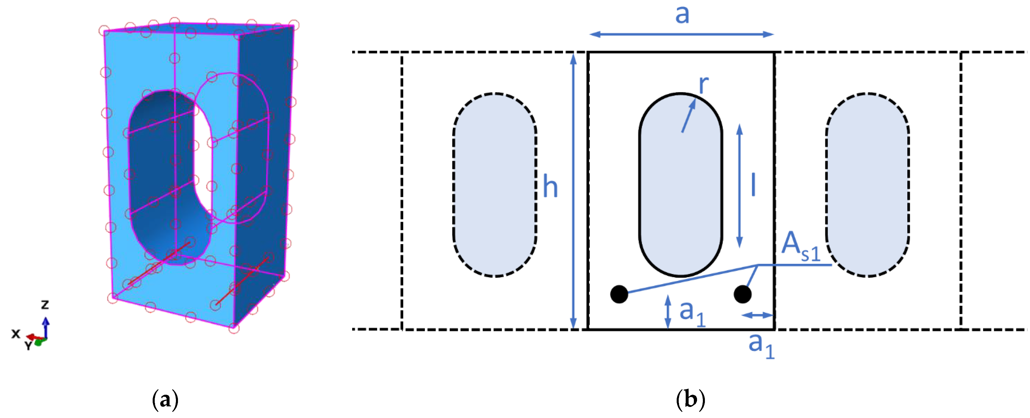
2.1. Representative Volume Element and Structure Parametrization

In this paper, the hollow core concrete slabs reinforced with steel bars are considered. The hollow cores are stadium shaped. The geometry of the structures replicates the commercial products of construction companies (manufacturers of prefabricated structures), which produces the precast HC slabs, for instance, SPK from Konbet [23] or HC from Pekabex [24]. The typical widths are 1200 mm and common heights of the slabs range from 150 to 500 mm, respectively.

Because the scope of the paper is to show the efficiency of the proposed problem reduction via an elaborate numerical approach, minor attention has been given to material modeling and linear elasticity was assumed. The typical values of the material constants have been used, namely, for concrete and steel, a Young’s modulus of 30 Gpa and 210 Gpa and Poisson’s ratio of 0.2 and 0.3 have been used, respectively.

Due to the homogenization method used, namely the Garbowski and Gajewski algorithm [9,10] it is necessary to isolate the representative volume element (RVE). The periodic geometry of HC slabs defines the RVE geometry which was used in a natural way. The width of the RVE slab corresponds to the vertical distances between the concrete ribs. Moreover, it was assumed that the RVE has a square base. The example of the RVE geometry is presented in Figure 2a. In the numerical homogenization technique used, the finite element (FE) stiffness matrix of the RVE must be computed; here, the Abaqus FEA was used for computing the stiffness matrix. The steel bars were modelled by using two-node, 3-dimenssional truss elements (T3D2 according to Abaqus FEA [25]), while the concrete volume was modelled by using solid general purpose linear brick elements with reduced integration (C3D8R according to Abaqus FEA [25]). These choices of element types are recommended and align with the best industry practices. Truss elements are particularly suitable for structures where the primary mode of load transfer is axial, such as in beams, columns, and trusses. Solid brick elements are well-suited for modeling concrete structures as they can capture both the tensile and compressive behaviors, as well as shear deformation and confinement effects. Moreover, the reduced integration helps to mitigate shear locking issues.

In the RVE, the reinforcement was taken into consideration by using a special numerical technique called embedded region [7,25]. In this technique, the interaction between steel and concrete is accounted for indirectly by using truss FE elements for modeling steel bars. Here, the stiffness of the steel truss FE is added to the concrete solid FE. In such an approach, an ideal bond between the materials is assumed. An alternative technique, not considered here, is the extrusion technique, in which steel is modeled by solid elements; the interaction is accounted by employing the contact techniques. The first approach is beneficial, because it does not require dense mesh in the area of the reinforcement and higher convergence is ensured.

In the study, the RVE is built based on the set of six parameters, which are simultaneously the ANN input parameters, see Figure 2b, i.e., $h$: slab height, $a$: width of a periodic part, $a_1$: position of the steel reinforcement, $r$: hole radius, $A_{s1}$: cross-sectional area of steel reinforcement and $l$: vertical dimension of the hole. The parameters having the greatest impact on the mechanical behavior of the HC slabs were selected (excluding material properties). They will have a direct impact on the laminate stiffnesses obtained from the numerical homogenization procedure, which form the output of the ANN. The ANN output is represented by the laminate mechanical properties matrix, explained in Section 2.3. In

Table 1. Assumed limits of the parameters of hollow core slabs.

Parameter	Symbol	Lower Boundary	Upper Boundary
Slab height	$h$ [cm]	15.0	50.0
Width of periodic part	$a$ [cm]	10.0	18.0
Position of the steel reinforcement	$a_1$ [cm]	2.0	3.0
Hole radius	$r$ [cm]	3.0	6.0
Cross-sectional area of steel reinforcement	$A_{s1}$ [cm2]	0.0	6.44
Vertical dimension of the hole	$l$ [cm]	0.0	20.0

, the lower and upper boundaries of the ANN input parameters assumed were demonstrated.

Based on the set of six parameters, the RVEs of HC slabs are built. Next, the computational FE mesh is automatically generated as the input for the Garbowski and Gajewski homogenization algorithm [10]. A few examples of the computational FE meshes used in the study are shown in Figure 3.

2.2. Latin Hypercube Sampling

In order to create a dataset for the artificial neural network, the Latin hypercube sampling method (LHS) according to McKay et al. [26] was used. The algorithm provides a large variety of near-random geometrical data from a multidimensional distribution for the RVE models that were used in the learning process of the ANN. Data was generated using Python library pyDOE2 [27]. In the library, various statistical functions are implemented to help the scientists, engineers and statisticians to construct experiments, mainly for creating factorization, response-surface or randomized experiments, such as LHS.

Let $n$ denote the intended number of the RVE models, and $k$ number of random geometrical parameters of the models. The sampling space is $k$-dimensional. There are two matrices: $n\times k$ matrix $\mathit{P}$ and $n\times k$ matrix $\mathit{R}$. In the matrix $\mathit{P}$, every $k$ column is a random permutation of $1,\dots ,n$. Matrix $\mathit{R}$ consists of the independent random values from the uniform distribution $\left(\mathrm{0,1}\right)$. Let us introduce $\mathit{V}$ matrix, in which every row contains input data for one RVE model. Sampling elements of matrix $\mathit{V}$ are defined as:

$$\mathit{V}=F^{-1}\left(\frac{{P_{ij}-R}_{ij}}{n}\right)$$

(1)

where $F^{-1}$ represents the inverse of the target cumulative distribution function.

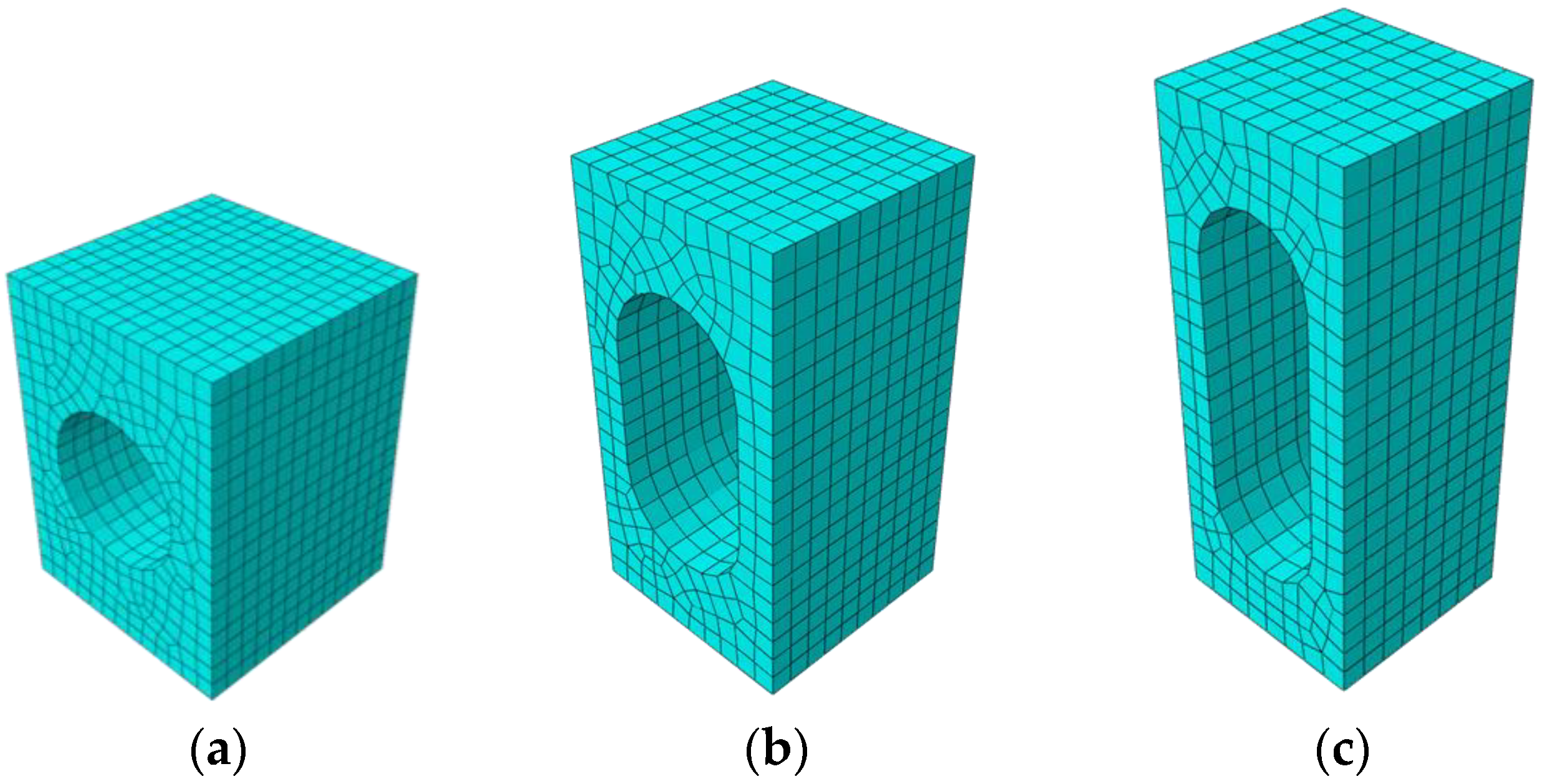
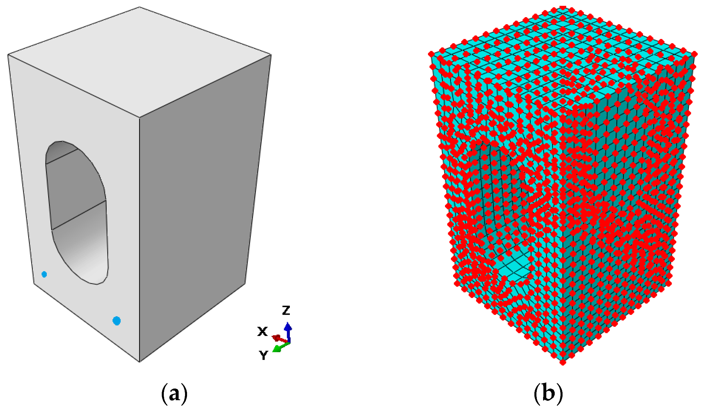
2.3. Numerical Homogenization of Precast Reinforced Concrete Slab

Within the framework of the research, one of the methods used was the Garbowski and Gajewski homogenization numerical technique [10]. The method is an extension of the proposal of Biancollini from 2004 [9]. The homogenization method is based on the deformation energy equivalent between a periodic section of a reinforced concrete hollow-core slab and a simplified two-dimensional shell element. Having on the one hand a representative volume element of a reinforced concrete hollow core slab with all geometric details and on the other hand a simplified shell model, the effective properties of the element can be determined assuming that the effective deformation in both models is equal. The reinforced concrete hollow-core slab is treated as a heterogeneous element, which consists of a concrete slab with circular or stadium openings and a layer of reinforcement with two bundles of steel rods. Reinforcement and openings are arranged along the y-direction, see Figure 4a.

Let us briefly introduce the homogenization method used. For more details, see [9,10]. In the finite element method, there is:

$${\mathit{K}}_{\mathit{e}}{·\mathit{u}}_{\mathit{e}}={\mathit{F}}_{\mathit{e}},$$

(2)

in which ${\mathit{K}}_{\mathit{e}}$ is a statically condensed (by eliminating the internal nodes) global stiffness matrix of a representative volumetric model, ${\mathit{u}}_{\mathit{e}}$ is a displacement vector of the external nodes, ${\mathit{F}}_{\mathit{e}}$ is a vector of nodal force applied to the external nodes. An example of the finite element mesh and external nodes is shown in Figure 4b.

The condensed stiffness matrix is calculated using the following equation:

$$\overline{\mathit{K}}={\mathit{K}}_{\mathit{e}\mathit{e}}-{\mathit{K}}_{\mathit{e}\mathit{i}}{\mathit{K}}_{\mathit{i}\mathit{i}}^{\mathbf{-}\mathbf{1}}{\mathit{K}}_{\mathit{i}\mathit{e}},$$

(3)

in which the overall stiffness matrix is decoupled by introducing the external (index $e$) and its internal (index $i$) nodes. Then, four submatrices may further be defined, which reads:

$$\left[\begin{array}{cc}{\mathit{K}}_{\mathit{e}\mathit{e}}& {\mathit{K}}_{\mathit{e}\mathit{i}}\\ {\mathit{K}}_{\mathit{i}\mathit{e}}& {\mathit{K}}_{\mathit{i}\mathit{i}}\end{array}\right]\left[\begin{array}{c}{\mathit{u}}_{\mathit{e}}\\ {\mathit{u}}_{\mathit{i}}\end{array}\right]=\left[\begin{array}{c}{\mathit{F}}_{\mathit{e}}\\ \mathbf{0}\end{array}\right].$$

(4)

After static condensation, the strain energy stored in the system is:

$$E=\frac{1}{2}{\mathit{u}}_{\mathit{e}}^{\mathit{T}}{\mathit{F}}_{\mathit{e}}.$$

(5)

The balance between the three-dimensional model and the shell model can be achieved by appropriate definition of displacements and rotations in external nodes.

Using the Mindlin-Reissner theory [28,29], the normal strain can be decomposed into a membrane and a bending state as follows:

$$\left[\begin{array}{c}{\epsilon }_x\\ {\epsilon }_y\\ {\gamma }_{xy}\end{array}\right]=\left[\begin{array}{c}\partial u/\partial x\\ \partial v/\partial y\\ \partial v/\partial x+\partial u/\partial y\end{array}\right]=\left[\begin{array}{c}{\epsilon }_x^0\\ {\epsilon }_y^0\\ {\gamma }_{xy}^0\end{array}\right]+z\left[\begin{array}{c}{\kappa }_x\\ {\kappa }_y\\ {\gamma }_{xy}\end{array}\right].$$

(6)

The relationship between the generalized deformations and the position of the nodes is expressed by the following transformation:

$${\mathit{u}}_i={\mathit{A}}_{\mathit{i}}{\mathit{ϵ}}_{\mathit{i}},$$

(7)

in which for a single $i$th node assuming $x_i=x$, $y_i=y$, $z_i=z$ we have:

$${\left[\begin{array}{c}{u}_x\\ u_y\\ u_z\end{array}\right]}_i={\left[\begin{array}{cccccccc}x& 0& y/2& z/2& 0& xz& 0& yz/2\\ 0& y& x/2& 0& z/2& 0& yz& xz/2\\ 0& 0& 0& x/2& y/2& -x^2/2& -y^2/2& -xy/2\end{array}\right]}_i{\left[\begin{array}{c}{\epsilon }_x\\ {\epsilon }_y\\ {\gamma }_{xy}\\ {\gamma }_{xz}\\ {\gamma }_{yz}\\ {\kappa }_x\\ {\kappa }_y\\ {\kappa }_{xy}\end{array}\right]}_i.$$

(8)

After substituting the above derivations into the definition of strain energy presented earlier in Equation (5), it can be obtained that:

$$E=\frac{1}{2}{\mathit{u}}_{\mathit{e}}^{\mathit{T}}\mathit{K}{\mathit{u}}_{\mathit{e}}=\frac{1}{2}{\mathit{ϵ}}_{\mathit{e}}^{\mathit{T}}{\mathit{A}}_{\mathit{e}}^{\mathit{T}}\mathit{K}{\mathit{A}}_{\mathit{e}}{\mathit{ϵ}}_{\mathit{e}}$$

(9)

and considering that for a shell element subjected to bending, tension/compression and transverse shearing, the internal energy finally takes the following form:

$$E=\frac{1}{2}{\mathit{ϵ}}_{\mathit{e}}^{\mathit{T}}{\mathit{A}}_{\mathit{k}}{ϵ}_e\left\{area\right\}.$$

(10)

The stiffness matrix for a shell element is calculated from the discrete matrix:

$${\mathit{A}}_{\mathit{k}}=\frac{{\mathit{A}}_{\mathit{e}}^{\mathit{T}}\overline{\mathit{K}}{\mathit{A}}_{\mathit{e}}}{area}.$$

(11)

From Equation (11), we obtain the laminate mechanical properties matrix ${\mathit{A}}_{\mathit{k}}$, also known in the literature as $\mathit{A}\mathit{B}\mathit{D}$ or $\mathit{A}\mathit{B}\mathit{D}\mathit{R}$ (with the extension of transverse shearing properties) matrix, in which:

$$\mathit{A}=\left[\begin{array}{ccc}{A}_{11}& A_{12}& 0\\ A_{21}& A_{22}& 0\\ 0& 0& A_{33}\end{array}\right]; \mathit{D}=\left[\begin{array}{ccc}{D}_{11}& D_{12}& 0\\ D_{21}& D_{22}& 0\\ 0& 0& D_{33}\end{array}\right],$$

(12)

$$\mathit{B}=\left[\begin{array}{ccc}{B}_{11}& B_{12}& 0\\ B_{21}& B_{22}& 0\\ 0& 0& B_{33}\end{array}\right];\mathit{R}=\left[\begin{array}{cc}{R}_{44}& 0\\ 0& R_{55}\end{array}\right].$$

(13)

Matrix $\mathit{A}$ determines compression/tension stiffnesses, matrix $\mathit{B}$ determines the coupling stiffnesses, matrix $\mathit{D}$ determines bending stiffnesses, while $\mathit{R}$ determines the transverse shear stiffnesses.

One also must determine the effective thickness of the shell, $t$, which can be obtained from the following equation:

$$t=\sqrt{12\frac{trace\left(\mathit{D}\right)}{trace\left(\mathit{A}\right)}}.$$

(14)

In Equation (14) it is assumed that the coordinate system is at the level of the neutral axis of the cross-section. If this is not true, the corrected value should be used, i.e., in the formula for $t$, instead of $\mathit{D}$, ${\mathit{D}}^{\mathit{*}}$ must be used, which takes ${\mathit{D}}^{\mathit{*}}=\mathit{D}-\mathit{B}{\mathit{A}}^{-1}\mathit{B}$ [13].

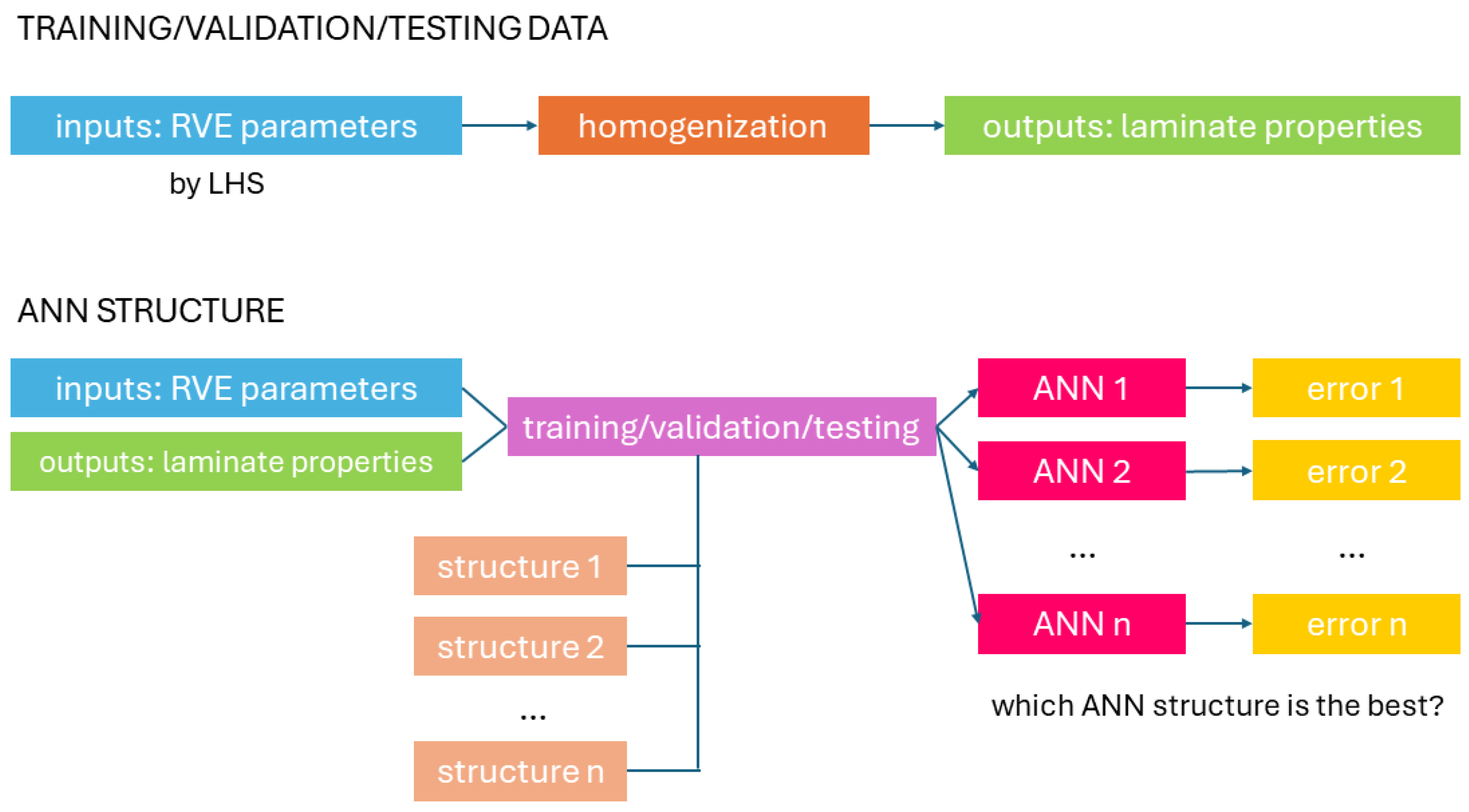
2.4. Artificial Neural Network

In this work, the Multi-Layer Perceptron Regressor (MLPRegressor) was used to create an artificial neural network model. MLPRegressor is an example of a deep learning algorithm. It learns non-linear functions and creates a map of the input data (geometric: dimensions of concrete slab, position of steel reinforcement, and physical: the area of the steel reinforcement, see Section 2.1) to the output data ($\mathit{A}\mathit{B}\mathit{D}\mathit{R}$ matrix, see Section 2.3) of the RVE models. In this study, MLPRegressor was used from scikit-learn [30]. Scikit-learn is a free, open-source machine learning library in Python. It features various machine learning algorithms, for instance, classification, regression, dimensionality reduction, model selection, pre-processing and clustering.

If there is a vector of the input data $\mathit{X}=x_1,x_2,\dots ,x_M$ and vector of the output data $y=y_1,y_2,\dots ,y_S$, where $M$ is the number of the input data, and $S$ is the number of the output data, MLPRegressor creates an estimation for the function $f\left(\cdot \right):\mathit{X}\to y$ for a regression problem. To create a model, it is required to define the number of the hidden neuron layers, the number of nodes in each of them, an activation function, and a solver for weight optimization. Multilayer perceptron may contain one or more hidden layers. Each node calculates the value from the previous node with the weight and deviation of that node. Nodes are connected with nodes in the next layer from input layer to the output. Data in the $j_n$ node is calculated by the following:

$$j_n=g\left(\sum _{i=1}^M{w}_{ij}{x}_i+b_j\right)$$

(15)

in which $g\left(\cdot \right)$ is a nonlinear activation function, $w_{ij}$ is a weight and $b_j$ is a deviation. MLPRegressor learns based on the expected results in the learning dataset by forward and backward propagation due to adjusting the weight of the connection $w_{ij}$ and values of deviation in the layer output $b_j$.

The activation function chosen for this research is Rectified Linear Unit (ReLU), which suits a lot of ANN models. The way the function ReLU is activated has a biological basis, namely, it is based on the behavior of the neurons in the brain. The activation function takes the following:

$$g\left({\rm X}\right)=max\left(0,\mathit{{\rm X}}\right).$$

(16)

The solver chosen for this research study is Adam [31]; it is easy to implement and efficient for the calculations for tasks characterized by a large amount of data and parameters. After [31], the pseudo code of the Adam algorithm was shown in Algorithm 1.

The Adam method, used for computing ANN weights, utilizes first and second moment vectors, which represents the estimation of the mean gradients and gradients variance, respectively. Beta parameters, ${\beta }_1$ and ${\beta }_2$, correct the first and second moments. Learning rates are adjusted adaptively for each parameter by dividing the current gradient by the square root of the current estimation of the second moment. With adaptive learning rate adjustment and the ability to use different coefficients for different parameters, Adam is more stable and efficient than traditional gradient-based optimization methods.

Algorithm 1. The pseudo code of the Adam algorithm.

1:$\mathrm{Require}: \alpha$ (stepsize) 2: $\mathrm{Require}: {\beta }_1,{\beta }_2\in \left[\mathrm{0,1}\right)$ (exponential decay rates for the moment estimates) 3: $\mathrm{Require}: f\left(\theta \right)$ (stochastic objective function with parameters $\theta$) 4: $\mathrm{Require}: {\theta }_0$ (initial parameter vector) 5: 6: $m_0\leftarrow 0$ (initialize $1\mathrm{s}\mathrm{t}$ moment vector) 7: $v_0 \leftarrow 0$ (initialize $2\mathrm{n}\mathrm{d}$ moment vector) 8: $t \leftarrow 0$ (initialize timestep) 9: 10: $while$ ${\theta }_t$ not converged $do$: 11:  $t \leftarrow t+1$ 12:  $g_t \leftarrow {\nabla }_{\theta }{f}_t\left({\theta }_{t-1}\right)$ 13:  $m_t \leftarrow {\beta }_1\cdot m_{t-1}+(1-{\beta }_1)\cdot g_t$ 14:  $v_t \leftarrow {\beta }_2\cdot v_{t-1}+(1-{\beta }_2)\cdot {g_t}^2$ 15:  ${\widehat{m}}_t \leftarrow m_t/(1-{{\beta }_1}^t)$ 16:  ${\widehat{v}}_t \leftarrow v_t/(1-{{\beta }_2}^t)$ 17:  ${\theta }_{t }\leftarrow {\theta }_{t-1 }-\alpha \cdot {\widehat{m}}_{t }/\left(\sqrt{{\widehat{v}}_{t }+ϵ}\right)$ 18: $end while$ 19: $return {\theta }_{t }v$

2.5. Error Measures

In order to estimate the quality of the implementation of the homogenization algorithm (see Section 3.1) or the quality of the approximation from ANN (see Section 3.3), its results were compared with the references, i.e., published in Garbowski and Gajewski’s paper [10] or computed by the homogenization algorithm implemented for this study research, respectively. Let us introduce the error, $e$, which is accounted by the following

$$e=\left|\frac{y-\overline{y}}{y}·100\%\right|,$$

(17)

in which $y$ is the reference, while $\overline{y}$ is the computed value.

Also, in order to compute the quality of ANN approximation by the scalar measure, the Mean Squared Error (MSE) was introduced. The MSE is accounted by the following

$$MSE=\frac{1}{10}\sum _{i=1}^{10}{\left(\mathit{A}\mathit{B}\mathit{D}{\mathit{R}}_{\mathit{i}}-{\overline{\mathit{A}\mathit{B}\mathit{D}\mathit{R}}}_{\mathbf{i}}\right)}^2 ,$$

(18)

in which, the vectors $\mathit{A}\mathit{B}\mathit{D}{\mathit{R}}_{\mathit{i}}$ and ${\overline{\mathit{A}\mathit{B}\mathit{D}\mathit{R}}}_{\mathbf{i}}$ are laminate theory stiffnesses vectors: $\{A_{11},A_{12},A_{22},A_{33},D_{11},D_{12},D_{22},D_{33}, R_{44}, R_{55}\}$, the reference obtained by numerical homogenization and the values derived by ANN approximation, respectively.

3. Results

3.1. Verification of the Implementation of the Homogenization Algorithm

The homogenization technique used in the study was implemented from scratch according to Garbowski and Gajewski’s paper [10] in the Python programming language. The mathematical details of the method were briefly introduced in Section 2.3. Here, the validation analysis was performed based on the numerical example from [10]. The example was computing the $\mathit{A}\mathit{B}\mathit{D}\mathit{R}$ matrix for the RVE of corrugated board with saw tooth geometry. The cardboard considered was a single-wall profile with three layers of paper. The axial spacing between the liners (outer layers of the cardboard) was 3.51 mm. The total thickness of the board was 3.8 mm. In the FE input model, the four-node quadrilateral elements with full integration scheme were used; this kind of element is labelled as S4 in Abaqus FEA [25]. These elements are recommended due to their versatility and effectiveness in structural analysis; they accurately model complex geometries and handle stress concentrations. The comparison between the results obtained from this study’s implementation and ref. [10] is presented in

Table 2. The stiffnesses of representative volume element of corrugated board with saw tooth geometry computed by numerical homogenization method from Python implementation confronted with data from Garbowski and Gajewski [10].

Effective Stiffness	Implementation of homogenization [10]	Published in [10]	Error
$A_{11} [\mathrm{k}\mathrm{P}\mathrm{a}\cdot \mathrm{m}]$	2139.7	2140.0	0.01%
$A_{22} [\mathrm{k}\mathrm{P}\mathrm{a}\cdot \mathrm{m}]$	1664.5	1665.0	0.03%
$A_{12} [\mathrm{k}\mathrm{P}\mathrm{a}\cdot \mathrm{m}]$	382.9	382.9	0.00% *
$A_{33} [\mathrm{k}\mathrm{P}\mathrm{a}\cdot \mathrm{m}]$	662.5	662.5	0.00% *
$D_{11} [\mathrm{P}\mathrm{a}\cdot {\mathrm{m}}^3]$	6.392	6.392	0.00% *
$D_{22} [\mathrm{P}\mathrm{a}\cdot {\mathrm{m}}^3]$	3.859	3.859	0.00% *
$D_{12} [\mathrm{P}\mathrm{a}\cdot {\mathrm{m}}^3]$	1.115	1.115	0.00% *
$D_{33} [\mathrm{P}\mathrm{a}\cdot {\mathrm{m}}^3]$	1.656	1.656	0.00% *
$R_{44} [\mathrm{P}\mathrm{a}\cdot \mathrm{m}]$	202.4	202.4	0.00% *
$R_{55}[\mathrm{P}\mathrm{a}\cdot \mathrm{m}]$	99.0	99.0	0.00% *

* within the considered accuracy.

. The effective stiffness considered, the value computed by the implemented Python algorithm, the value from [10] and the value of error are presented in the columns of the table, respectively. The error was computed according to the formula presented in Section 2.5.

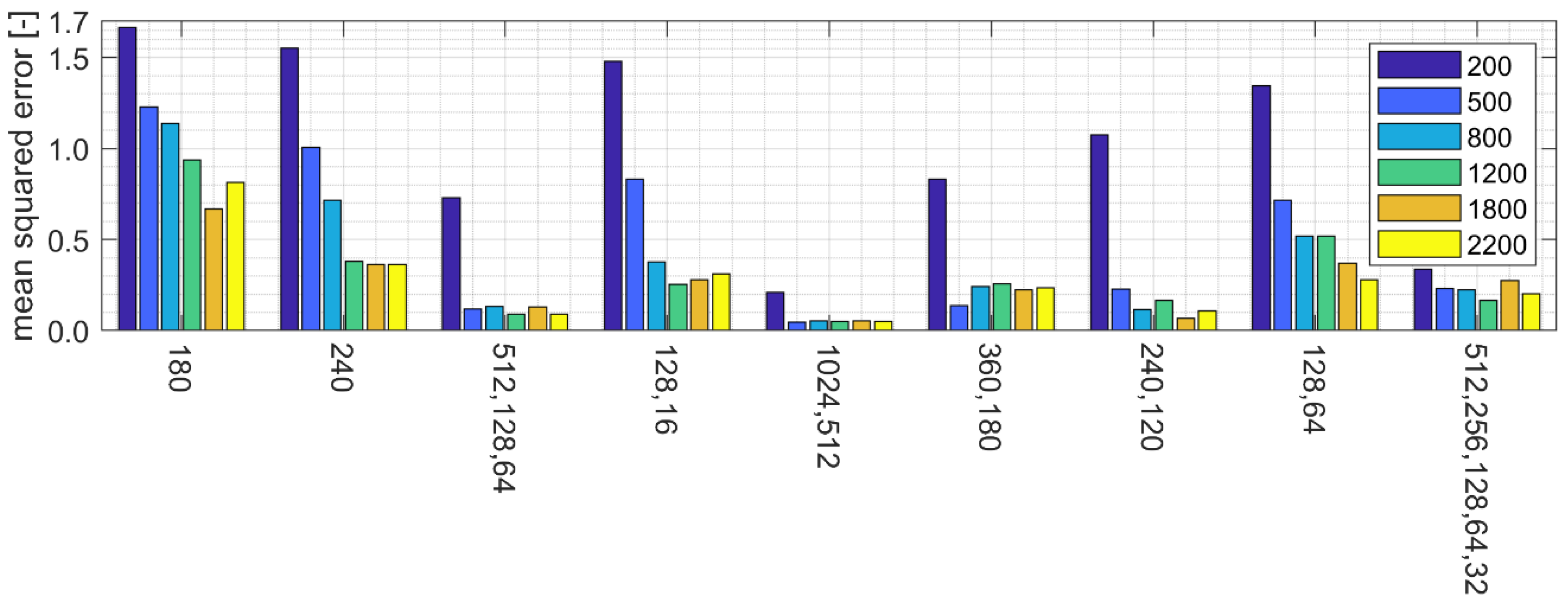
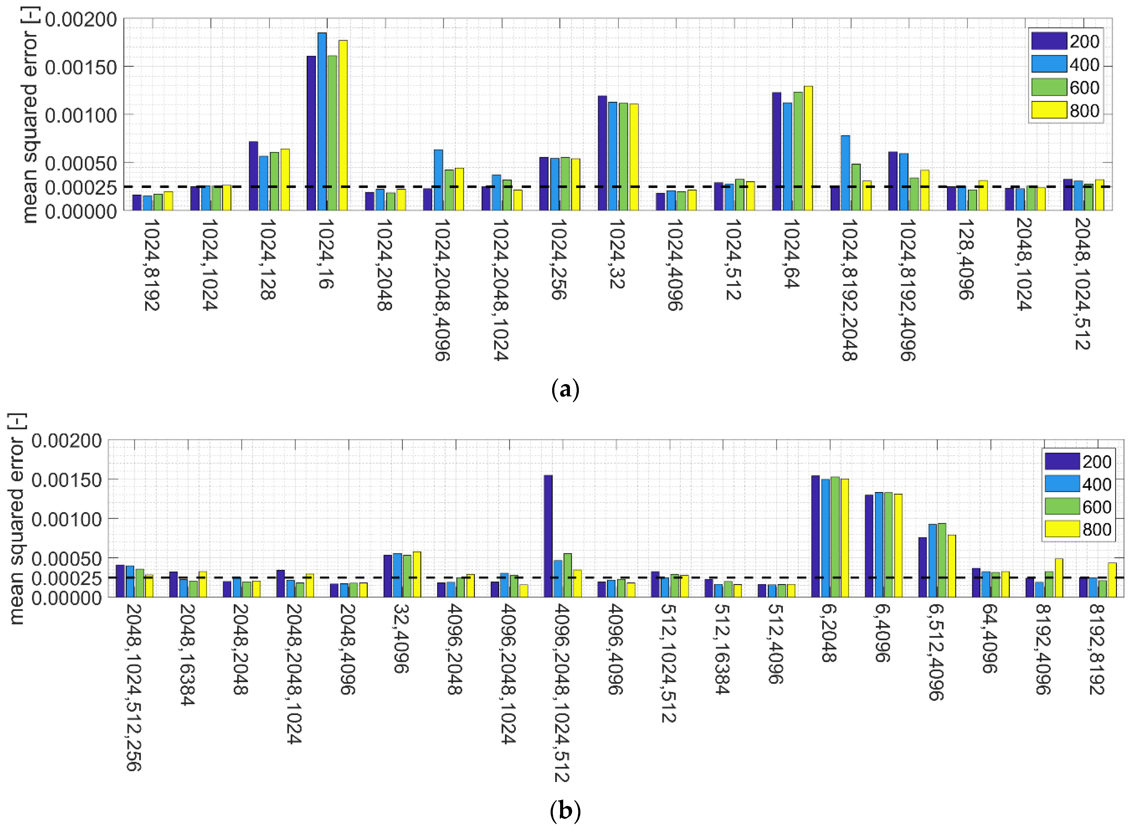
3.2. Selection of Parameter Values of the Artificial Neural Network Due to Approximation Error

The values of parameters of the ANN which would ensure high accuracy of ANN approximation are not trivial to define. In general, learning time and the accuracy of the approximation obtained depends on many variables, such as solver of the algorithm, number of neurons in layers, number of epochs, data size and format or difficulty of the problem (number of inputs/outputs). Therefore, in this study, an analysis of ANN performance due to selected parameters has been conducted. The main goal was to obtain a configuration with the smallest error measured by the MSE, see Section 2.5. Each ANN configuration was used 10 times and the average MSE was calculated for each configuration. In order to accelerate the calculations and reduce the MSE, the data were rescaled for the learning process. In each instance of ANN, the parameters to decide were (1) the number of layers, (2) the number of neurons in each layer and (3) the number of epochs. The number of layers used were limited from one to four. The number of neurons was from 32 to 8192. The number of epochs considered were from 200 to 2200.

The net was tested on six models (independent from the training set). Obviously, overfitting is one of the most common concerns; here, the typical approach was used, namely, the validation set was observed during training and was stopped if the validation set error increased.

In the research study, first, several ANN configurations were selected and ANNs were trained with these configurations. The result of this preliminary study is presented in Figure 5. The horizontal tick labels represents the number of neurons and number of layers. For example, “128,16” represents a two-layer case, with 128 neurons in the first layer and 16 in the second layer, respectively. Next, with better insight into what determines lower error of ANN approximation for the problem of HC reinforced concrete slabs, the further ANN configurations were selected to find ANN cases with lower error. The most interesting cases and those with the lowest error were selected and shown in Figure 6.

3.3. Achieved Accuracy of the Artificial Neural Network

In this section, the result of ANN approximation with its best configuration found was validated with the results of traditional calculations, i.e., without the use of ANN, but with the use of Garbowski and Gajewski’s algorithm [10]. As can be concluded by analyzing the graphs in Figure 5 and Figure 6, the best results, i.e., those with the lowest MSE, were obtained by a two-layer network with 1024 and 8192 neurons. The model of this network was used to compare the results from ANN with the results from the homogenization algorithm.

Six examples were selected to show the actual performance of the best ANN. The parameters of six examples of RVE considered are presented in

Table 3. Six examples of parameter sets for testing the accuracy of the best artificial neural network.

Example	$\mathit{h}$ [cm]	$\mathit{a}$ [cm]	${\mathit{a}}_1$ [cm]	$\mathit{r}$ [cm]	${\mathit{A}}_{\mathit{s}1}$ [cm2]	$\mathit{l}$ [cm]
1	45.338	17.958	2.654	4.427	5.024	6.205
2	41.454	17.497	2.763	4.304	2.804	0.707
3	49.704	15.191	2.657	3.811	4.233	17.965
4	34.155	17.209	2.167	4.550	1.800	12.737
5	43.766	17.278	2.747	5.624	3.490	9.842
6	42.823	17.736	2.273	5.964	3.034	4.266

. They were generated randomly within the considered parameter limits, see Table 1, assuming a homogeneous sampling distribution. The results from best ANN are summarized in

Table 4. Comparison of the effective stiffnesses for the first example.

Effective Stiffness	ANN Homogenization	Homogenization [10]	Error
$A_{11} [\mathrm{k}\mathrm{P}\mathrm{a}\cdot \mathrm{m}]$	109.0	109.1	0.09%
$A_{22} [\mathrm{k}\mathrm{P}\mathrm{a}\cdot \mathrm{m}]$	130.1	132.0	1.44%
$A_{12} [\mathrm{k}\mathrm{P}\mathrm{a}\cdot \mathrm{m}]$	25.53	25.52	0.04%
$A_{33} [\mathrm{k}\mathrm{P}\mathrm{a}\cdot \mathrm{m}]$	44.68	44.61	0.16%
$D_{11} [\mathrm{P}\mathrm{a}\cdot {\mathrm{m}}^3]$	0.2419	0.2441	0.9%
$D_{22} [\mathrm{P}\mathrm{a}\cdot {\mathrm{m}}^3]$	0.2613	0.2697	3.11%
$D_{12} [\mathrm{P}\mathrm{a}\cdot {\mathrm{m}}^3]$	0.0543	0.0545	0.37%
$D_{33} [\mathrm{P}\mathrm{a}\cdot {\mathrm{m}}^3]$	0.0949	0.0952	0.32%
$R_{44} [\mathrm{P}\mathrm{a}\cdot \mathrm{m}]$	36.15	36.2	0.14%
$R_{55} [\mathrm{P}\mathrm{a}\cdot \mathrm{m}]$	41.08	40.86	0.54%

,

Table 5. Comparison of the effective stiffnesses for the second example.

Effective Stiffness	ANN Homogenization	Homogenization [10]	Error
$A_{11} [\mathrm{k}\mathrm{P}\mathrm{a}\cdot \mathrm{m}]$	113.7	113.8	0.09%
$A_{22} [\mathrm{k}\mathrm{P}\mathrm{a}\cdot \mathrm{m}]$	126.8	126.4	0.32%
$A_{12} [\mathrm{k}\mathrm{P}\mathrm{a}\cdot \mathrm{m}]$	26.72	26.74	0.07%
$A_{33} [\mathrm{k}\mathrm{P}\mathrm{a}\cdot \mathrm{m}]$	45.29	45.3	0.02%
$D_{11} [\mathrm{P}\mathrm{a}\cdot {\mathrm{m}}^3]$	0.1867	0.1896	1.53%
$D_{22} [\mathrm{P}\mathrm{a}\cdot {\mathrm{m}}^3]$	0.2011	0.2007	0.2%
$D_{12} [\mathrm{P}\mathrm{a}\cdot {\mathrm{m}}^3]$	0.0419	0.0422	0.71%
$D_{33} [\mathrm{P}\mathrm{a}\cdot {\mathrm{m}}^3]$	0.0734	0.0738	0.54%
$R_{44} [\mathrm{P}\mathrm{a}\cdot \mathrm{m}]$	37.34	37.41	0.19%
$R_{55} [\mathrm{P}\mathrm{a}\cdot \mathrm{m}]$	39.57	39.76	0.48%

,

Table 6. Comparison of the effective stiffnesses for the third example.

Effective Stiffness	ANN Homogenization	Homogenization [10]	Error
$A_{11} [\mathrm{k}\mathrm{P}\mathrm{a}\cdot \mathrm{m}]$	90.64	90.33	0.34%
$A_{22} [\mathrm{k}\mathrm{P}\mathrm{a}\cdot \mathrm{m}]$	125.8	127.6	1.41%
$A_{12} [\mathrm{k}\mathrm{P}\mathrm{a}\cdot \mathrm{m}]$	21.23	21.1	0.62%
$A_{33} [\mathrm{k}\mathrm{P}\mathrm{a}\cdot \mathrm{m}]$	39.05	39.1	0.13%
$D_{11} [\mathrm{P}\mathrm{a}\cdot {\mathrm{m}}^3]$	0.2946	0.2967	0.71%
$D_{22} [\mathrm{P}\mathrm{a}\cdot {\mathrm{m}}^3]$	0.3296	0.3396	2.94%
$D_{12} [\mathrm{P}\mathrm{a}\cdot {\mathrm{m}}^3]$	0.0667	0.067	0.45%
$D_{33} [\mathrm{P}\mathrm{a}\cdot {\mathrm{m}}^3]$	0.1164	0.1173	0.77%
$R_{44} [\mathrm{P}\mathrm{a}\cdot \mathrm{m}]$	31.09	30.88	0.68%
$R_{55} [\mathrm{P}\mathrm{a}\cdot \mathrm{m}]$	40.50	40.64	0.34%

,

Table 7. Comparison of the effective stiffnesses for the fourth example.

Effective Stiffness	ANN Homogenization	Homogenization [10]	Error
$A_{11} [\mathrm{k}\mathrm{P}\mathrm{a}\cdot \mathrm{m}]$	50.32	50.08	0.48%
$A_{22} [\mathrm{k}\mathrm{P}\mathrm{a}\cdot \mathrm{m}]$	79.67	77.78	2.43%
$A_{12} [\mathrm{k}\mathrm{P}\mathrm{a}\cdot \mathrm{m}]$	11.3	11.25	0.44%
$A_{33} [\mathrm{k}\mathrm{P}\mathrm{a}\cdot \mathrm{m}]$	23.26	23.19	0.3%
$D_{11} [\mathrm{P}\mathrm{a}\cdot {\mathrm{m}}^3]$	0.0831	0.0859	3.26%
$D_{22} [\mathrm{P}\mathrm{a}\cdot {\mathrm{m}}^3]$	0.1001	0.0992	0.91%
$D_{12} [\mathrm{P}\mathrm{a}\cdot {\mathrm{m}}^3]$	0.0182	0.0186	2.15%
$D_{33} [\mathrm{P}\mathrm{a}\cdot {\mathrm{m}}^3]$	0.035	0.0352	0.57%
$R_{44} [\mathrm{P}\mathrm{a}\cdot \mathrm{m}]$	14.63	14.58	0.34%
$R_{55} [\mathrm{P}\mathrm{a}\cdot \mathrm{m}]$	22.54	22.68	0.62%

,

Table 8. Comparison of the effective stiffnesses for the fifth example.

Effective Stiffness	ANN Homogenization	Homogenization [10]	Error
$A_{11} [\mathrm{k}\mathrm{P}\mathrm{a}\cdot \mathrm{m}]$	82.52	82.4	0.15%
$A_{22} [\mathrm{k}\mathrm{P}\mathrm{a}\cdot \mathrm{m}]$	106.0	106.1	0.09%
$A_{12} [\mathrm{k}\mathrm{P}\mathrm{a}\cdot \mathrm{m}]$	18.9	18.89	0.05%
$A_{33} [\mathrm{k}\mathrm{P}\mathrm{a}\cdot \mathrm{m}]$	34.36	34.2	0.47%
$D_{11} [\mathrm{P}\mathrm{a}\cdot {\mathrm{m}}^3]$	0.2069	0.206	0.44%
$D_{22} [\mathrm{P}\mathrm{a}\cdot {\mathrm{m}}^3]$	0.2274	0.2275	0.04%
$D_{12} [\mathrm{P}\mathrm{a}\cdot {\mathrm{m}}^3]$	0.0461	0.0456	1.1%
$D_{33} [\mathrm{P}\mathrm{a}\cdot {\mathrm{m}}^3]$	0.0817	0.0812	0.62%
$R_{44} [\mathrm{P}\mathrm{a}\cdot \mathrm{m}]$	25.55	25.42	0.51%
$R_{55} [\mathrm{P}\mathrm{a}\cdot \mathrm{m}]$	31.31	31.36	0.16%

and

Table 9. Comparison of the effective stiffnesses for the sixth example.

Effective Stiffness	ANN Homogenization	Homogenization [10]	Error
$A_{11} [\mathrm{k}\mathrm{P}\mathrm{a}\cdot \mathrm{m}]$	94.79	94.91	0.13%
$A_{22} [\mathrm{k}\mathrm{P}\mathrm{a}\cdot \mathrm{m}]$	112.5	112.5	0.0% *
$A_{12} [\mathrm{k}\mathrm{P}\mathrm{a}\cdot \mathrm{m}]$	21.88	21.86	0.09%
$A_{33} [\mathrm{k}\mathrm{P}\mathrm{a}\cdot \mathrm{m}]$	38.43	38.43	0.0% *
$D_{11} [\mathrm{P}\mathrm{a}\cdot {\mathrm{m}}^3]$	0.1997	0.2025	1.38%
$D_{22} [\mathrm{P}\mathrm{a}\cdot {\mathrm{m}}^3]$	0.2162	0.2179	0.78%
$D_{12} [\mathrm{P}\mathrm{a}\cdot {\mathrm{m}}^3]$	0.0447	0.0449	0.45%
$D_{33} [\mathrm{P}\mathrm{a}\cdot {\mathrm{m}}^3]$	0.0786	0.0792	0.76%
$R_{44} [\mathrm{P}\mathrm{a}\cdot \mathrm{m}]$	29.69	29.65	0.13%
$R_{55} [\mathrm{P}\mathrm{a}\cdot \mathrm{m}]$	33.55	33.54	0.03%

* within the considered accuracy.

. The effective stiffnesses considered, the value computed by the best ANN, the values from the use of Garbowski and Gajewski’s homogenization algorithm [10] and the values of error were presented in the columns, respectively. The errors were computed according to the formula presented in Section 2.5.

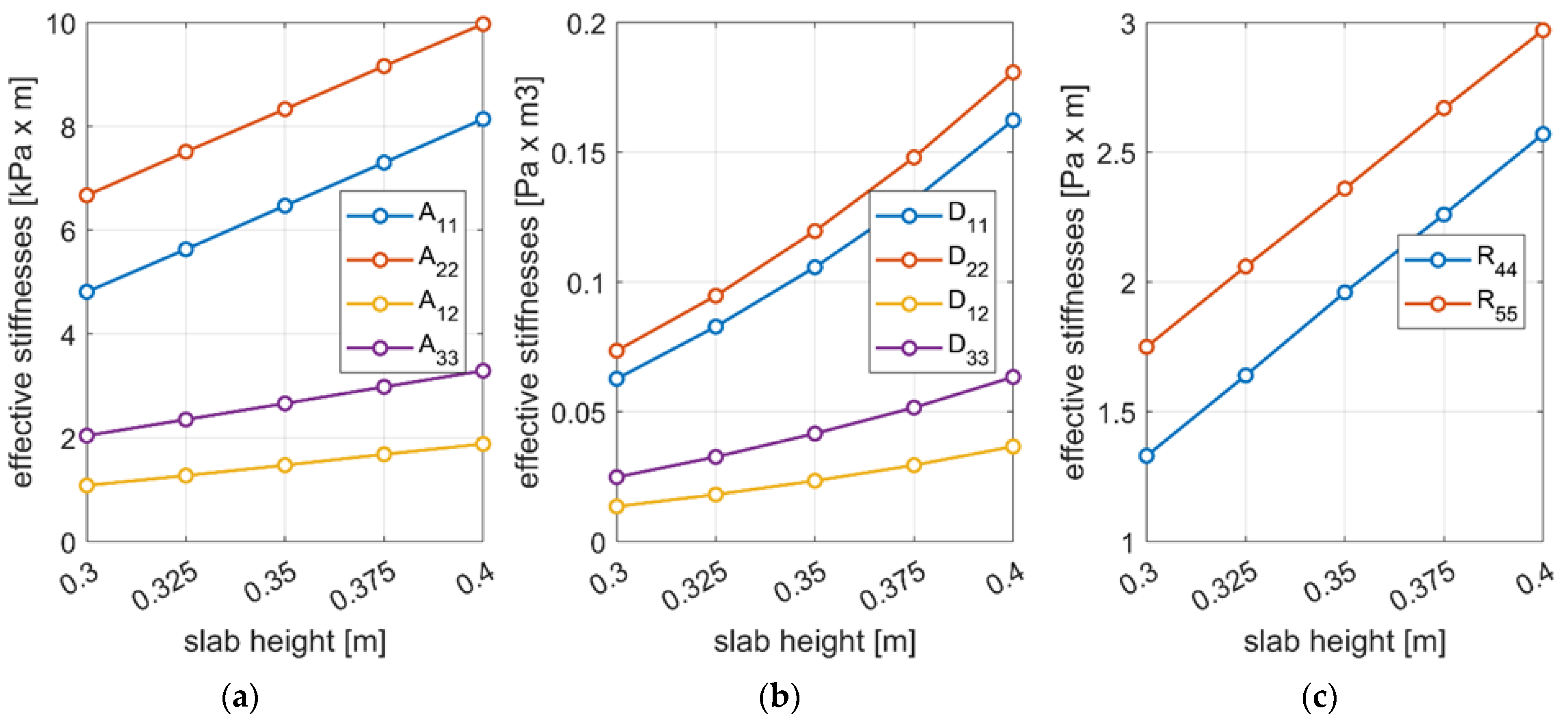
3.4. Influence of Changing Parameters of Prefabricated Concrete Slabs on the Effective Stiffnesses

Having a trained and accurate ANN which represents the properties of the prefabricated HC concrete slabs through RVE response from numerical homogenization, the influence of particular parameter of the slab structure can be verified. For example, by modifying one parameter in a certain range of values, we can check changes in RVE effective properties. To present such an example, the parameter of height, $h$, was selected due to its large influence on compression/tension stiffnesses of RVE. The slab height $h$ was changed from 0.3 m to 0.4 m with a step of 0.025 m. The other parameters were fixed: $a=$ 0.14 m, $a_1=$0.025 m, $r=$0.05 m, $A_{s1}=$ 0.00038 m² and $l=$ 0.07 m. ANN calculations were then performed to obtain the effective and representative properties of five cases of prefabricated slabs with different heights. The summary of the results were presented in

Table 10. Effect of increasing the height of a precast concrete slab model on the effective stiffnesses of a representative volume element.

Effective Stiffnesses	h [m]
	0.300	0.325	0.350	0.375	0.400
$A_{11} [\mathrm{k}\mathrm{P}\mathrm{a}\cdot \mathrm{m}]$	4.81	5.63	6.47	7.30	8.14
$A_{22} [\mathrm{k}\mathrm{P}\mathrm{a}\cdot \mathrm{m}]$	6.67	7.51	8.33	9.16	9.97
$A_{12} [\mathrm{k}\mathrm{P}\mathrm{a}\cdot \mathrm{m}]$	1.08	1.27	1.47	1.68	1.88
$A_{33} [\mathrm{k}\mathrm{P}\mathrm{a}\cdot \mathrm{m}]$	2.04	2.35	2.66	2.98	3.29
$D_{11} [\mathrm{P}\mathrm{a}\cdot {\mathrm{m}}^3]$	0.0627	0.0828	0.1057	0.1318	0.1623
$D_{22} [\mathrm{P}\mathrm{a}\cdot {\mathrm{m}}^3]$	0.0735	0.0947	0.1196	0.1480	0.1808
$D_{12} [\mathrm{P}\mathrm{a}\cdot {\mathrm{m}}^3]$	0.0135	0.0181	0.0234	0.0294	0.0366
$D_{33} [\mathrm{P}\mathrm{a}\cdot {\mathrm{m}}^3]$	0.0248	0.0326	0.0416	0.0516	0.0634
$R_{44} [\mathrm{P}\mathrm{a}\cdot \mathrm{m}]$	1.33	1.64	1.96	2.26	2.57
$R_{55} [\mathrm{P}\mathrm{a}\cdot \mathrm{m}]$	1.75	2.06	2.36	2.67	2.97

. The table illustrates the predicted effective properties of RVE due to the use of an artificial neural network depending on the given height of the slab model. Not only membrane, but also bending and transverse shearing properties were shown. In Figure 7, the same data are presented using curves grouped by property type (membrane, bending or transverse shearing).

4. Discussion

Soft computing methods applied in mechanical engineering problems may greatly reduce the size of the problems considered without losing the accuracy of the solution. In this paper, it was proven that the artificial neural network applied to the engineering problem may be an interesting alternative to consider by the designers instead of using design standards.

First, in Section 3.1, the homogenization method implemented was validated with the scientific paper. The example considered was replicated from the literature after [10] and it proved a faultless implementation of the method in the Python environment as presented in Table 2. In the table, the last column shows the errors computed as shown in Section 2.5. The values achieved are very low, and in most cases they are even equal to 0 within the assumed precision.

Secondly, in Section 3.2, the configuration of the ANN with the best performance was sought. More than one hundred and fifty configurations were analyzed; selected cases are presented in Figure 5 and Figure 6. From the presented configurations, the best ones were selected on the basis of the error measurement according to the MSE measure from Section 2.5. As shown in Figure 6a, the best results were obtained by the model with two hidden layers with 1024 and 8192 neurons (400 epochs), in which the accuracy was 0.00017. This model was used to compare the results from ANN and homogenization algorithm in next section, i.e., Section 3.3. Moreover, based on the results obtained it was observed that the ANN with one layer of neurons always was characterized with high MSE. Those ANN configurations are not recommended to be used.

In general, the more neurons, the better the accuracy. For example, if the total number of neurons was greater than 8000, the MSE obtained was no higher than 0.0005. However, also for a smaller total number of neurons, low MSE could be obtained, e.g., for the “4096, 512” ANN configuration, the MSE was 0.00018, which was one of the best results. Also, the “1024, 2048” ANN configuration gave a low MSE, i.e., 0.0002, while “1024, 1024” gave a MSE equal to 0.00025. These four values can be thought of as a Pareto front when considering the number of neurons and the MSE accuracy.

In this study, the influence of a number of epochs was also verified. It was observed that increasing the number of epochs significantly affects the MSE if a small number of total neurons is considered, see Figure 5. MSE can be decreased even several times, like in “128, 64”, in which the MSE for 2200 epochs was almost five times lower than for 200 epochs. Similar features may be observed for the “512, 128, 64” configuration. However, that feature does not occur if the total number of neurons is higher, see Figure 6, i.e., for 1000 or more of total neurons, the fluctuations are not so significant and the trend is not always preserved. For instance, in the best case, “1024, 8192”, the relation is the opposite; for 200 epochs, the MSE is 0.00016, while for 800 epochs the MSE equals 0.00019. It should be emphasized that the overfitting effect may occur for a large number of epochs. Therefore, an ANN with a lower epoch number should be preferred when comparing two ANN configurations with similar errors.

The verification of the values of the effective stiffnesses were also computed in Section 3.3 for selected cases, see Table 3. In the first example, the greatest error was equal to 3.11% and 1.44%, while the rest was not greater than 0.6%. In the second example, the greatest error was equal to 1.5%, while the rest was not greater than 0.7%. In the third example, the greatest error was equal to 2.9% and 1.41%, while the rest was not greater than 0.8%. In the fourth example, the greatest error was equal to 3.26%, 2.43% and 2.15% while the rest was not greater than 1.0%. In the fifth example, the greatest error was equal to 1.1% and 0.62%, while the rest was not greater than 0.51%. In the sixth example, the greatest error was equal to 1.38%, 0.78% and 0.76%, while the rest was not greater than 0.45%. Individual effective stiffnesses with high error values were not observed. As shown above, for random examples selected, the biggest error was 3.11%, which proves very good agreement between the value computed by trained ANN and the value computed due to homogenization algorithm [10]. Those magnitudes of values of error in homogenization computations are acceptable as shown in [12,18].

Having a quick and reliable approximation of the RVE properties of prefabricated hollow-core slabs makes it possible to analyze the effect of changing the parameters on the individual mechanical properties of this complex structure. The example of such analysis was shown in this study, see Section 3.4. In Table 10 and Figure 7, the effect of changing the height of the prefabricated slab on its effective stiffnesses, i.e., compression/tension, bending and transversal shear stiffnesses was demonstrated. Other parameters of RVE were fixed. In Figure 7a, it may be observed that the influence on $A_{11}$, $A_{22}$, $A_{12}$ and $A_{33}$ is linear. For those properties, the maximal increase of the height, i.e., 33%, causes the increase of 69%, 49%, 74% and 61% of the effective stiffnesses, respectively. The influence is one and a half times greater, taking into account $D_{11}$, $D_{22}$, $D_{12}$ and $D_{33}$, the values are increased with 159%, 146%, 171% and 156% for 0.4 m slab height, respectively. The trends for $D$ stiffnesses are slightly nonlinear, see Figure 7b. While considering the transversal shear stiffnesses, i.e., $R_{44}$ and $R_{55}$, the growths are linear, see Figure 7c. The percentage increases for 0.4 m slab height are 93% and 70%, respectively. The above analysis of five examples was derived from ANN computations which took less than 0.1 s.

The ANN model built in the study gives the computational results in a very short time. The numerical homogenization for 50 models takes about 26 min, while for 200 models it is about 104 min. The ANN computations for 50 models last about 0.6 s, while for 200 models it lasts 0.75 s. The time saving while comparing the homogenization method and ANN computations is several thousand times.

There are a few limitations of the study, namely, relatively simple measure for error was used for training the ANN. In the literature, there are a lot of other functions, which may reduce the probability of overfitting. Also, for finding the solution with lower MSE, the trial-and-error method was used. One can utilize a more elaborate method to determine the number of layers and neurons through solving formal optimization problem. However, it should be properly conditioned to avoid overfitting. Other more advanced ANN architectures such as convolutional, recurrent networks or physics-based neural networks [18,32] were not explored in the study. The application of such architectures or the use of other machine learning regressors could improve accuracy and/or generalizability and could be included in future studies. Furthermore, in the study, the experimental validation was not conducted. The Authors refer directly to the homogenization method results, the effectiveness of which has already been confirmed in the literature, therefore, no validation is required. The main aim of the study is to replace the computations of homogenization according to laminate theory with an ANN approach and find its best structure. Therefore, to demonstrate the effectiveness of the proposed approach, the numerical examples provided were sufficient.

5. Conclusions

In this study, the soft computing technique was used to build the surrogate model for numerical homogenization in order to rapidly characterize the mechanical properties of hollow core reinforced concrete slabs depending on the slab properties. First, the homogenization technique based on the strain energy equivalence between the numerical three-dimensional model with geometrical details of the HC slab and its representation of Reissner-Mindlin flat plate was implemented and validated. Second, the framework of the artificial neural network was developed with automatic generation of RVE with given parameters. Next, the ANN was trained to compute the effective stiffnesses of shell representation of HC slab based on several geometrical parameters.

An important part of the study was the performance analysis of ANN. The performance of the network was checked for a selected numbers of epochs, the number of hidden layers and number of neurons. The accuracy of the approximation was measured by using the mean squared error. The network achieved the highest accuracy for 200 epochs and two hidden layers (1024 and 8196 neurons). The average calculation times were also compared; in the case of calculations using ANN, the cost was several thousand times lower than that while using homogenization method.

References

1. Derkowski, W.; Surma, M. Prestressed hollow core slabs for topped slim floors—Theory and research of the shear capacity. Eng. Struct. 2021, 241, 112464. [Google Scholar] [CrossRef]
2. Jankowiak, T.; Łodygowski, T. Identification of parameters of concrete damage plasticity constitutive model. Found. Civ. Environ. Eng. 2005, 6, 53–69. [Google Scholar]
3. Hafezolghorani Esfahani, M.; Hejazi, F.; Vaghei, R.; Jaafar, M.; Karimzadeh, K. Simplified Damage Plasticity Model for Concrete. Struct. Eng. Int. 2017, 27, 68–78. [Google Scholar] [CrossRef]
4. Lubliner, J.; Oliver, J.; Oller, S.; Oñate, E. A plastic-damage model for concrete. Int. J. Solids Struct. 1989, 25, 299–326. [Google Scholar] [CrossRef]
5. Chrysanidis, T.A.; Panoskaltsis, V.P. Experimental investigation on cracking behavior of reinforced concrete tension ties. Case Stud. Constr. Mater. 2022, 16, e00810. [Google Scholar] [CrossRef]
6. Vu, K.A.T.; Stewart, M.G. Predicting the likelihood and extent of reinforced concrete corrosion-induced cracking. J. Struct. Eng. 2005, 131, 1681–1689. [Google Scholar] [CrossRef]
7. Arab, A.A.; Badie, S.S.; Manzari, M.T. A methodological approach for finite element modeling of pretensioned concrete members at the release of pretensioning. Eng. Struct. 2011, 33, 1918–1929. [Google Scholar] [CrossRef]
8. Staszak, N.; Garbowski, T.; Ksit, B. Application of the generalized nonlinear constitutive law in numerical analysis of hollow-core slabs. Arch. Civ. Eng. 2022, 68, 125–145. [Google Scholar] [CrossRef]
9. Biancolini, M.E. Evaluation of equivalent stiffness properties of corrugated board. Comp. Struct. 2005, 69, 322–328. [Google Scholar] [CrossRef]
10. Garbowski, T.; Gajewski, T. Determination of transverse shear stiffness of sandwich panels with a corrugated core by numerical homogenization. Materials 2021, 14, 1976. [Google Scholar] [CrossRef]
11. Kalita, K.; Haldar, S.; Chakraborty, S. A Comprehensive Review on High-Fidelity and Metamodel-Based Optimization of Composite Laminates. Arch. Comput. Methods Eng. 2022, 29, 3305–3340. [Google Scholar] [CrossRef]
12. Staszak, N.; Szymczak-Graczyk, A.; Garbowski, T. Elastic Analysis of Three-Layer Concrete Slab Based on Numerical Homogenization with an Analytical Shear Correction Factor. Appl. Sci. 2022, 12, 9918. [Google Scholar] [CrossRef]
13. Staszak, N.; Garbowski, T.; Szymczak-Graczyk, A. Solid Truss to Shell Numerical Homogenization of Prefabricated Composite Slabs. Materials 2021, 14, 4120. [Google Scholar] [CrossRef]
14. Archaviboonyobul, T.; Chaveesuk, R.; Singh, J.; Jinkarn, T. An analysis of the influence of hand hole and ventilation hole design on compressive strength of corrugated fiberboard boxes by an artificial neural network model. Packag. Technol. Sci. 2020, 33, 171–181. [Google Scholar] [CrossRef]
15. Adamopoulos, S.; Anthony, K.; Rapti, E.; Birbilis, D. Predicting the properties of corrugated base papers using multiple linear regression and artificial neural networks. Drewno 2016, 59, 61–72. [Google Scholar] [CrossRef]
16. Gajewski, T.; Grabski, J.K.; Cornaggia, A.; Garbowski, T. On the use of artificial intelligence in predicting the compressive strength of various cardboard packaging. Packag. Technol. Sci. 2023, 37, 97–105. [Google Scholar] [CrossRef]
17. Stręk, A.M.; Dudzik, M.; Kwiecień, A.; Wańczyk, K.; Lipowska, B. Verification of application of ANN modelling in study of compressive behaviour of aluminium sponges. Eng. Trans. 2019, 67, 271–288. [Google Scholar] [CrossRef]
18. Garbowski, T.; Knitter-Piątkowska, A.; Grabski, J.K. Estimation of the Edge Crush Resistance of Corrugated Board Using Artificial Intelligence. Materials 2023, 16, 1631. [Google Scholar] [CrossRef]
19. Gajewski, T.; Staszak, N.; Garbowski, T. Parametric optimization of thin-walled 3D beams with perforation based on homogenization and soft computing. Materials 2022, 15, 2520. [Google Scholar] [CrossRef]
20. Adamski, M.; Czechlowski, M.; Durczak, K.; Garbowski, T. Determination of the Concentration of Propionic Acid in an Aqueous Solution by POD-GP Model and Spectroscopy. Energies 2021, 14, 8288. [Google Scholar] [CrossRef]
21. Araujo, G.; Andrade, F.A.A. Post-Processing Air Temperature Weather Forecast Using Artificial Neural Networks with Measurements from Meteorological Stations. Appl. Sci. 2022, 12, 7131. [Google Scholar] [CrossRef]
22. Mrówczyński, D.; Gajewski, T.; Garbowski, T. Sensitivity Analysis of Open-Top Cartons in Terms of Compressive Strength Capacity. Materials 2023, 16, 412. [Google Scholar] [CrossRef]
23. Konbet. Dokumentacja Techniczna Sprężone Płyty Kanałowe SPK 15, SPK 20, SPK 26.5, SPK 32, SPK 40, SPK 50. Brochure. Available online: https://www.konbet.com.pl/pliki/Plyty-stropowe-kanalowe-strunobetonowe-SPK_dokumentacja-techniczna.pdf (accessed on 15 February 2023).
24. Pekabex. Hollow Core Slab 265. Datasheet. Available online: https://pekabex.pl/wp-content/files/HC265.pdf (accessed on 15 February 2023).
25. Dassault Systèmes. Abaqus Documentation. 2019. Available online: https://abaqusdocs.mit.edu/ (accessed on 15 February 2024).
26. McKay, M.D.; Beckman, R.J.; Conover, W.J. A Comparison of Three Methods for Selecting Values of Input Variables in the Analysis of Output from a Computer Code. Technometrics 1979, 42, 55–61. [Google Scholar] [CrossRef]
27. Python Library pyDOE2 1.3.0. 2021. Available online: https://pypi.org/project/pyDOE2/ (accessed on 15 June 2021).
28. Mindlin, R.D. Influence of Rotatory Inertia and Shear De-formation on Flexural Motion of Isotropic, Elastic Plates. J. Appl. Mech. 1951, 18, 31–38. [Google Scholar] [CrossRef]
29. Reissner, E. The Effect of Transverse Shear Deformation on the Bending of Elastic Plates. ASME J. Appl. Mech. 1945, 12, 69–77. [Google Scholar] [CrossRef]
30. Python Library Scikit-Learn 1.2.1. 2021. Available online: https://scikit-learn.org/stable/ (accessed on 15 June 2021).
31. Kingma, D.P.; Ba, J.L. Adam: A Method for Stochastic Optimization. In Proceedings of the 3rd International Conference for Learning Representations (ICLR), San Diego, CA, USA, 7–9 May 2015. [Google Scholar]
32. Rogalka, M.; Grabski, J.K.; Garbowski, T. A Comparison of Two Artificial Intelligence Approaches for Corrugated Board Type Classification. Eng. Proc. 2023, 56, 272. [Google Scholar] [CrossRef]
Figure 1. The flowchart graphically representing the research study.
Applsci 14 03018 g001
Figure 2. (a) The representative volume element of the section of the hollow-core slab with host part (blue volume contour) and submerged elements of reinforcement (red lines); (b) scheme of a cross-section of a hollow core concrete slab with the parameters of a representative volume element.
Applsci 14 03018 g002
Figure 3. Selected examples of the generated computational mesh of hollow core slabs used as a representative volume element: (a) slab with circular hole, (b,c) slabs with different stadium type holes.
Applsci 14 03018 g003
Figure 4. Representative volume element: (a) model with reinforcement indicated in blue and (b) mesh of the model with marked external nodes in red.
Applsci 14 03018 g004
Figure 5. Mean squared errors for selected ANN configurations in the preliminary stage of the study for different epochs.
Applsci 14 03018 g005
Figure 6. Mean squared errors for selected ANN configurations for different epochs.
Applsci 14 03018 g006
Figure 7. The plots of effects of increasing the height of a precast concrete slab model on the effective stiffness of a representative volume element in: (a) compression/tension (b) bending and (c) transverse shearing.
Applsci 14 03018 g007