


Global Maximum Power Point Tracking of a Photovoltaic Module Array Based on Modified Cat Swarm Optimization


Abstract
1. Introduction
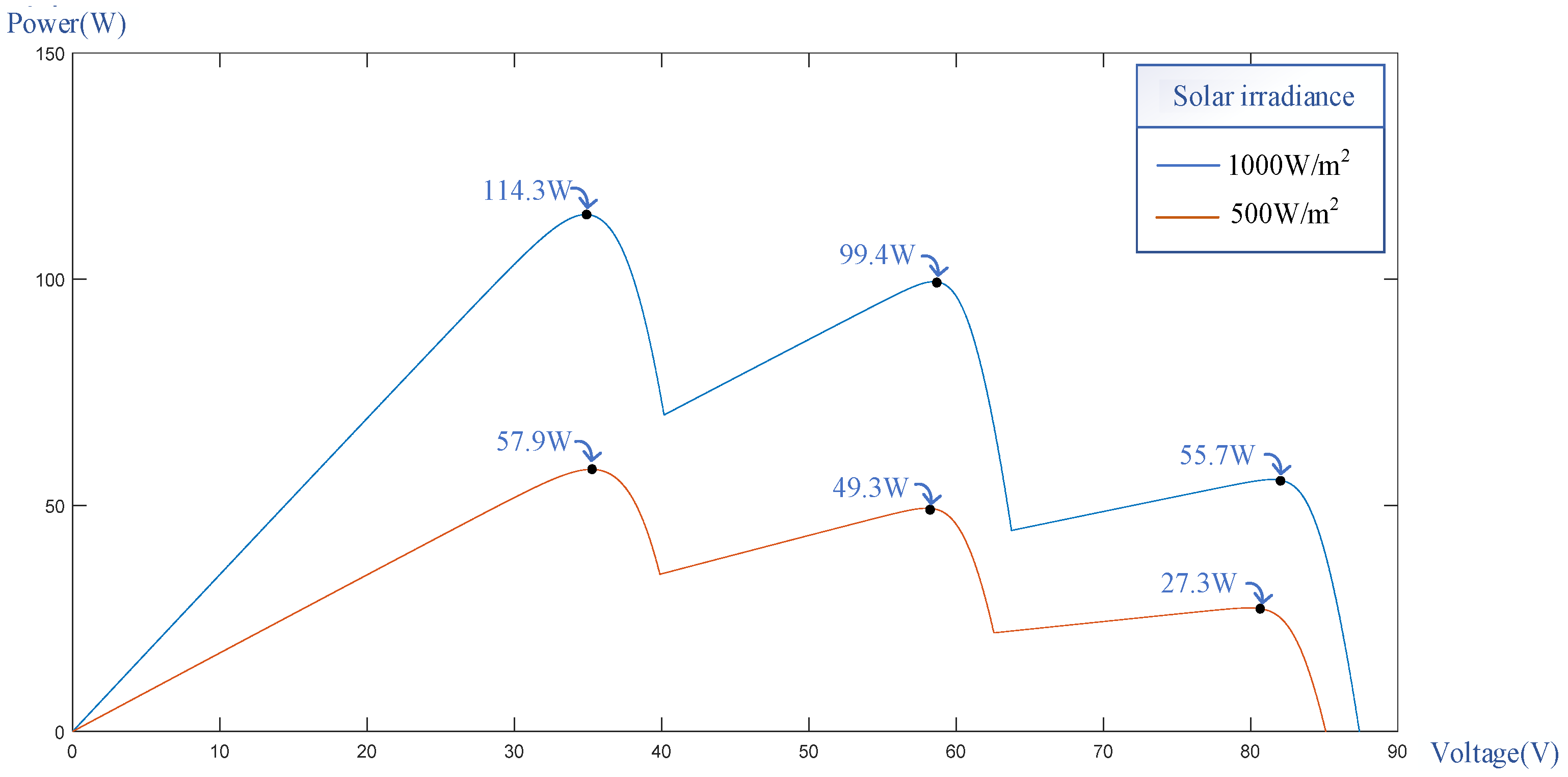
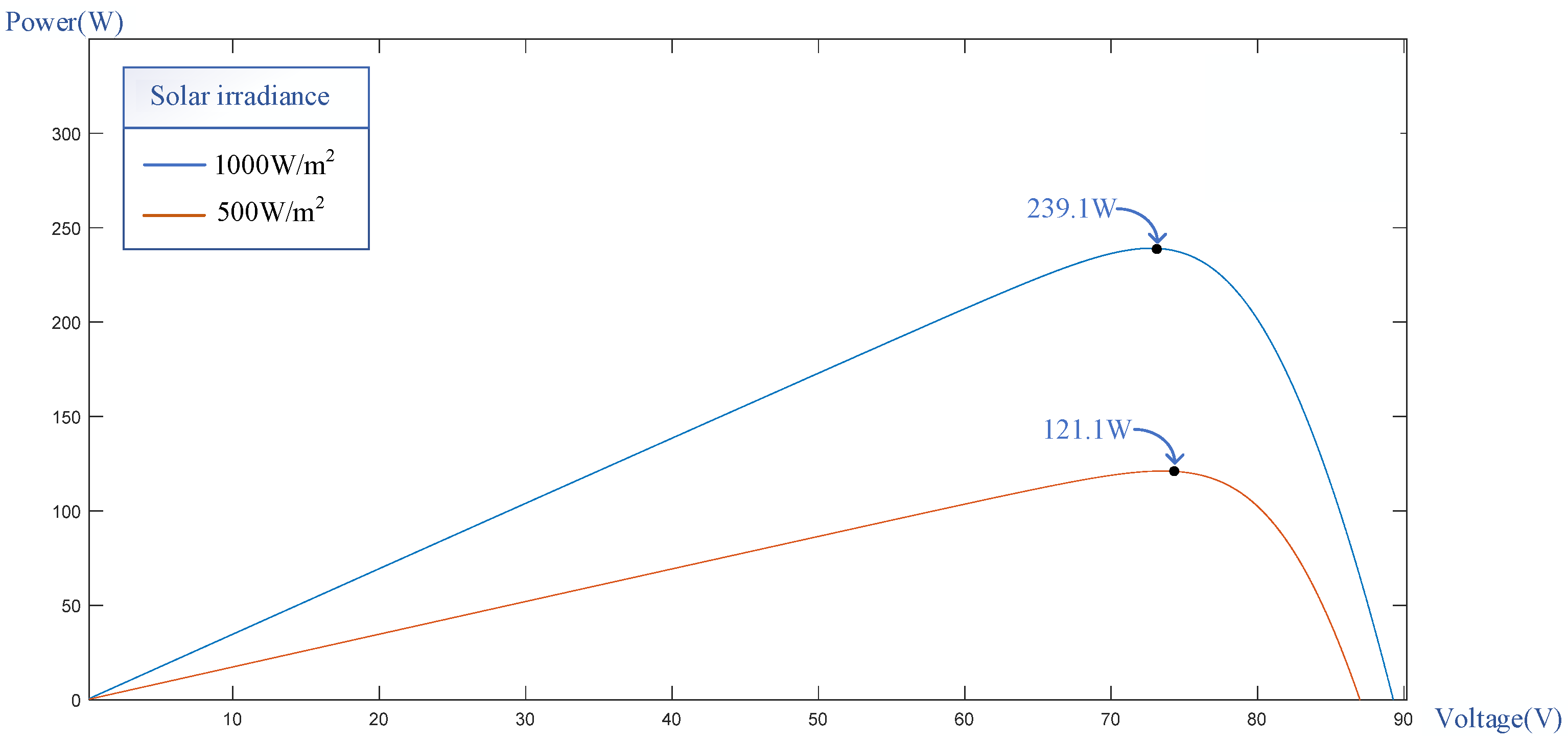
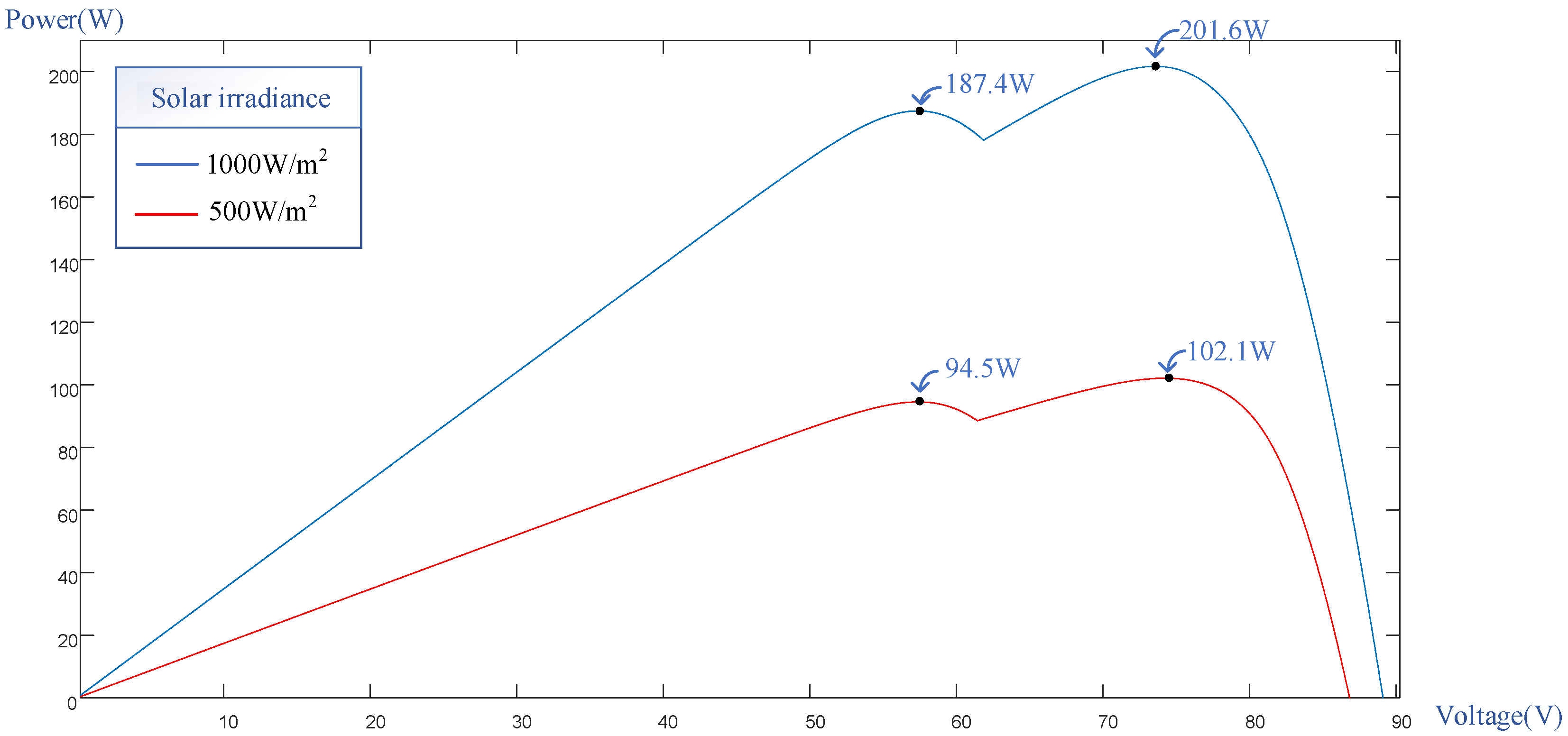
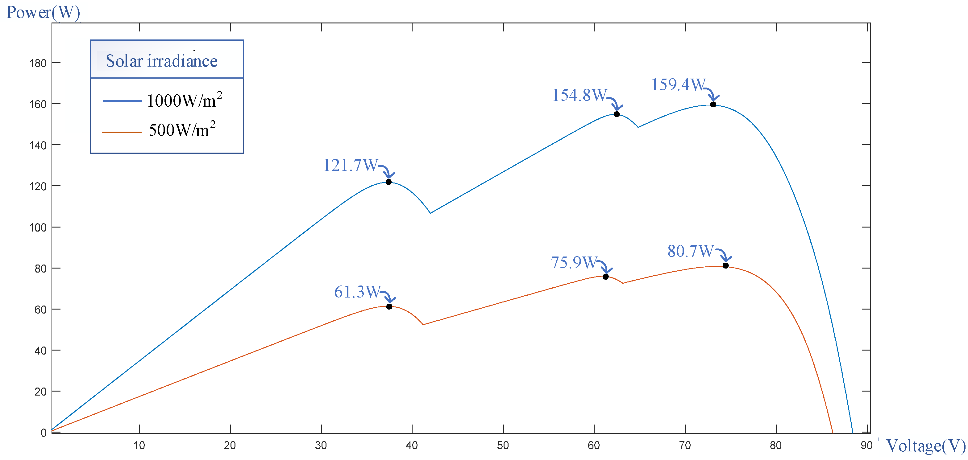
2. PVMA Output Characteristics under Different Shading Conditions
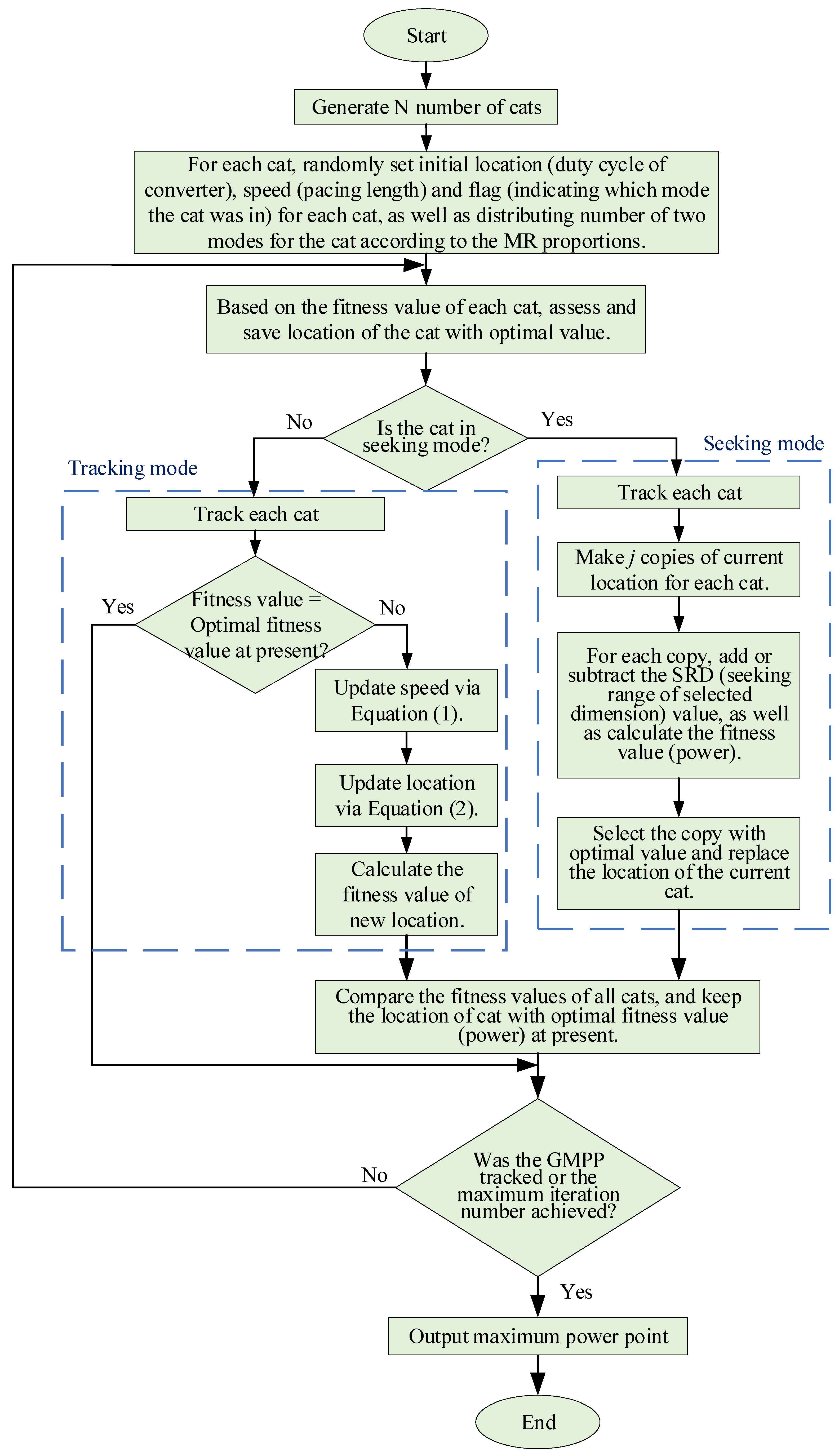
3. Conventional Cat Swarm Optimization
- Cat quantity: This ensures the number of cats needed for the algorithm, which affects the converging capability and speed of CSO. In this study, we used 6 cats.
- Initial location (duty cycle of converter): The initial location of each cat should be set right from the start; in this study, they were set randomly.
- Speed (tracking pace): After setting the initial location, the initial speed can be calculated accordingly.
- Cat flag: This parameter refers to the Boolean value indicated with only “yes” or “no”. “Yes” means that the cat is in seeking mode and “no” means that the cat is in tracking mode.
- Maximum number of iterations: The condition for iteration termination was set here to ensure that the CSO operation would cease within a certain time frame.
3.1. Seeking Mode
3.2. Tracking Mode
- Update tracking speed vi according to Equation (1):
- 2.
- Update cat location xi according to Equation (2):where is the location of cat i after update; is the location of cat i before update; is the tracking speed of cat i after update; and is the current iteration number (t = 1–30).
4. Proposed MCSO
4.1. MCSO with Fixed Initial Tracking Voltage
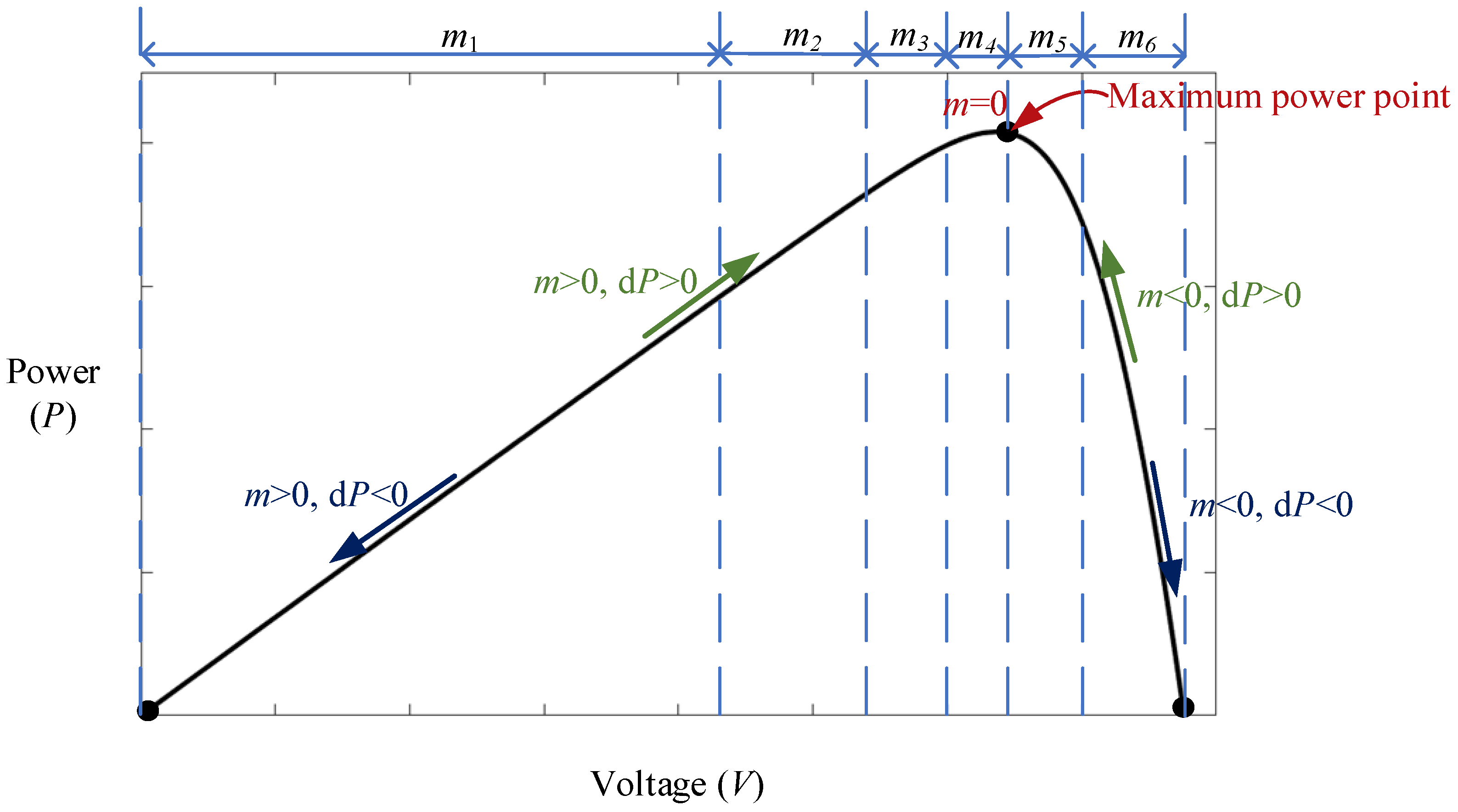
4.2. MCSO with Fixed Initial Tracking Voltage Combined with Tracking Pace Adjusted with Slope of P-V Curve
- (1)
- When slope m is less than zero, it indicates that the system has tracked to the right side of the MPP, and the tracking direction is heading toward the MPP at the left.
- (2)
- When slope m is greater than zero, it indicates that the system has tracked to the left side of the MPP, and the tracking direction is heading toward the MPP at the right.
- (3)
- When slope m is zero, it indicates that the system has tracked the MPP. The slope (m) and power variation (dP) are defined by Equations (3) and (4), respectively:
4.3. MCSO with Fixed Initial Tracking Voltage Combined with Tracking Pace Adjusted by Inertia Weight
4.4. MCSO with Fixed Initial Tracking Voltage Combined with Tracking Pace Adjusted by the Slope of P-V Curve and Inertia Weight
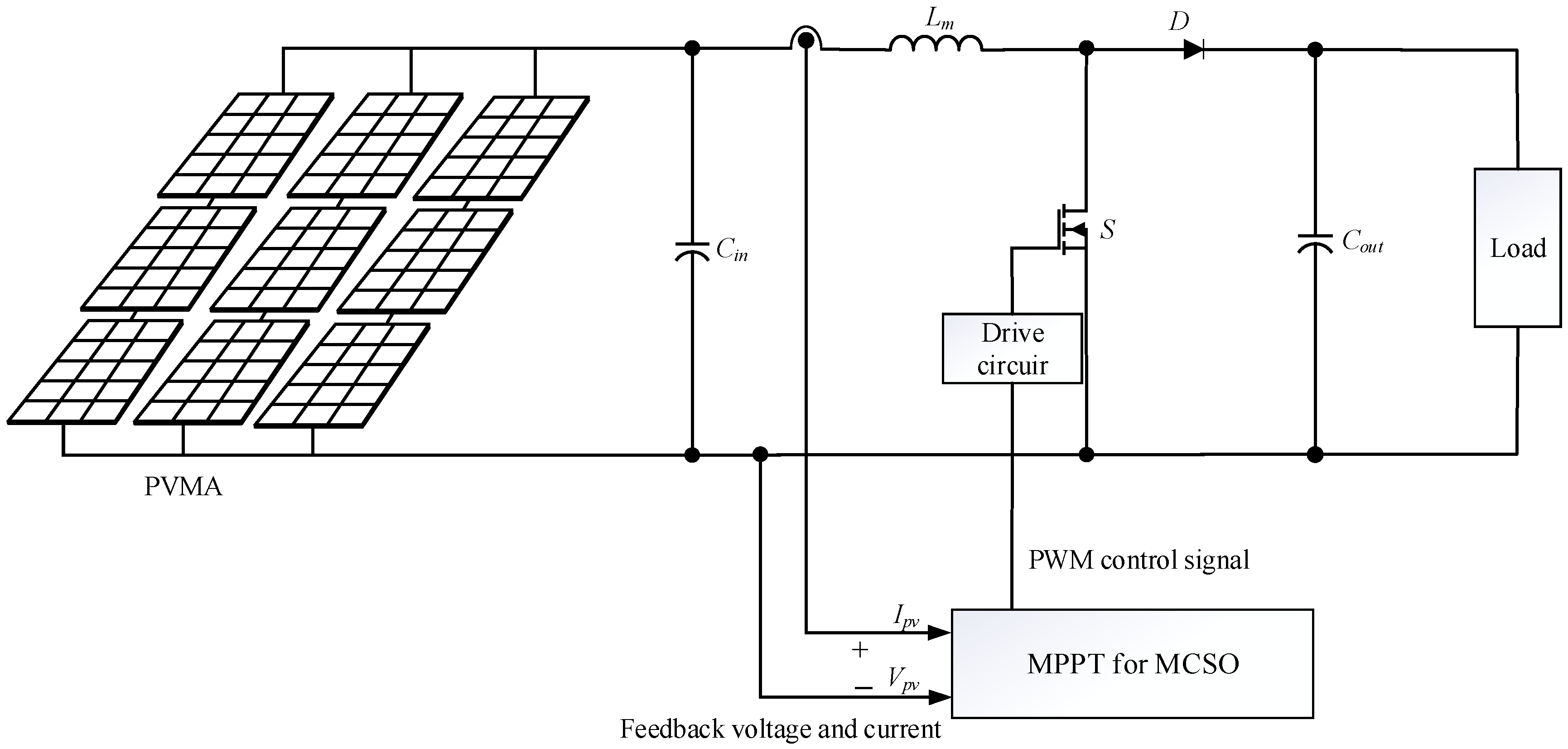
5. Design of MPPT Controlling Converter
6. Simulated Results
- (1)
- Test of Case 1
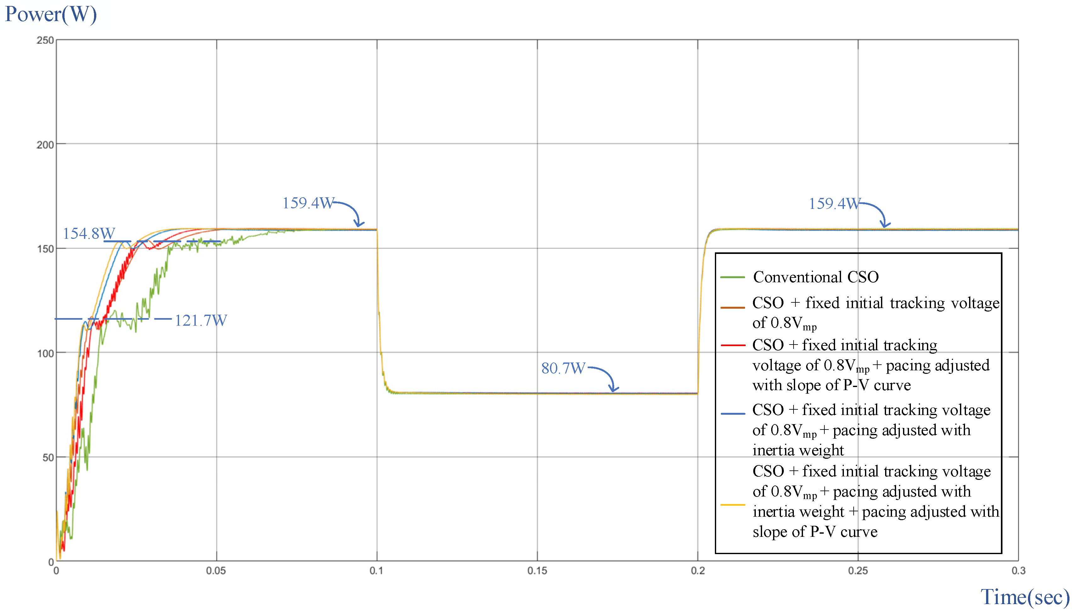
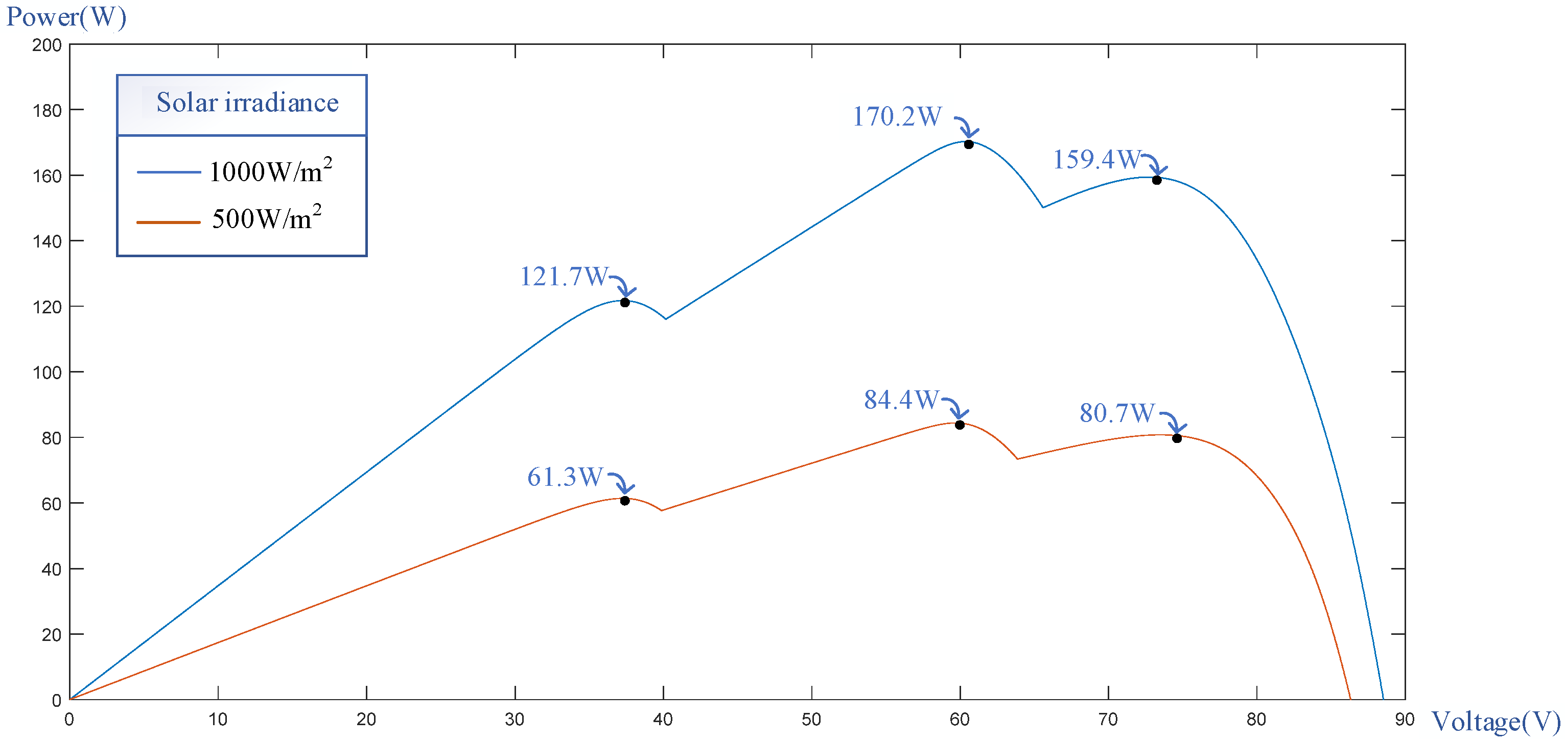
- (2)
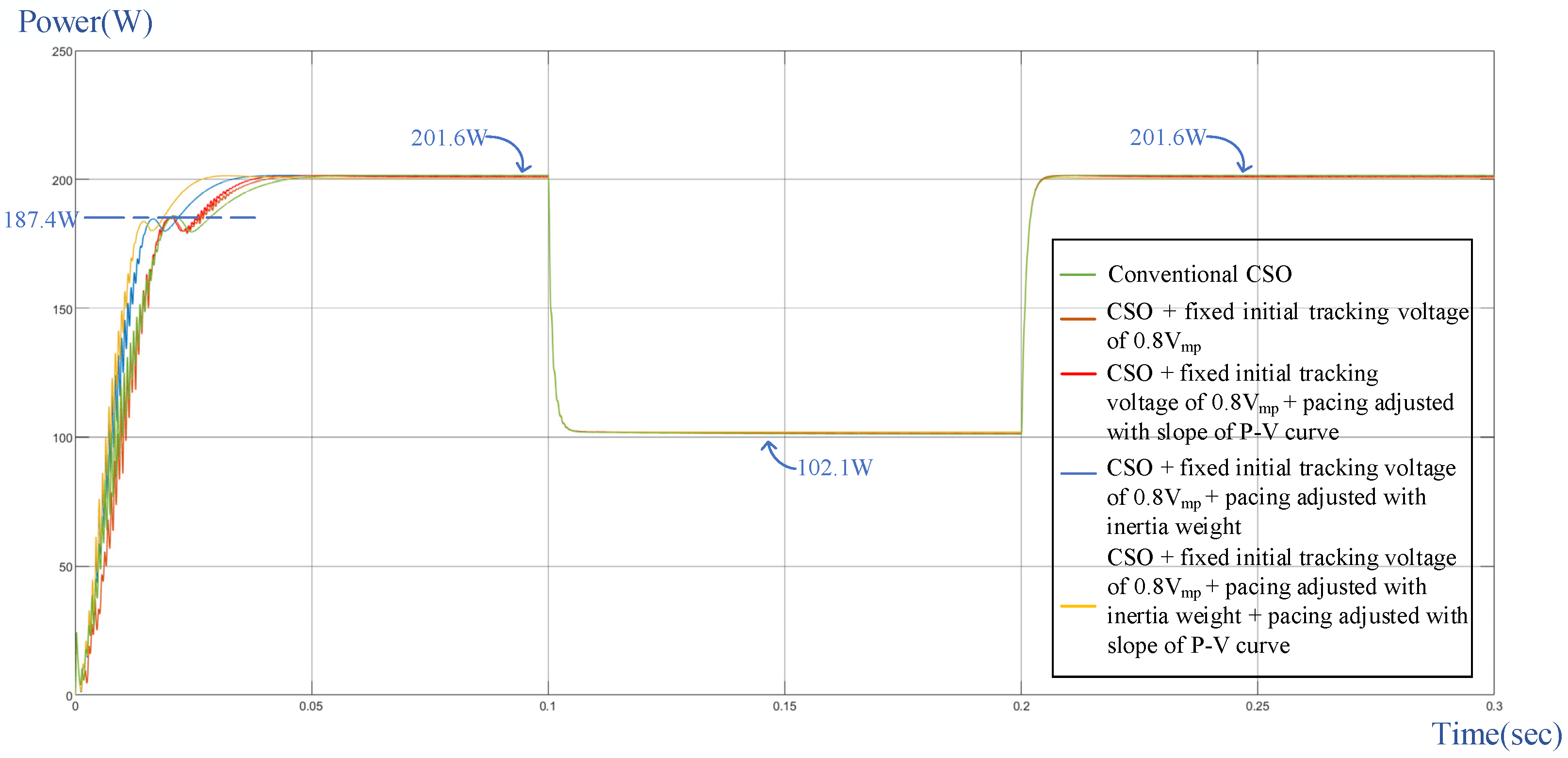
- Test of Case 2
- (3)
- Test of Case 3
- (4)
- Test of Case 4
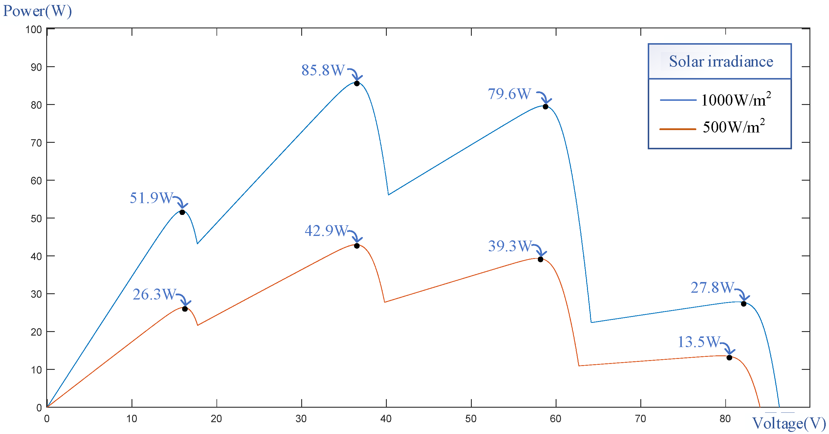
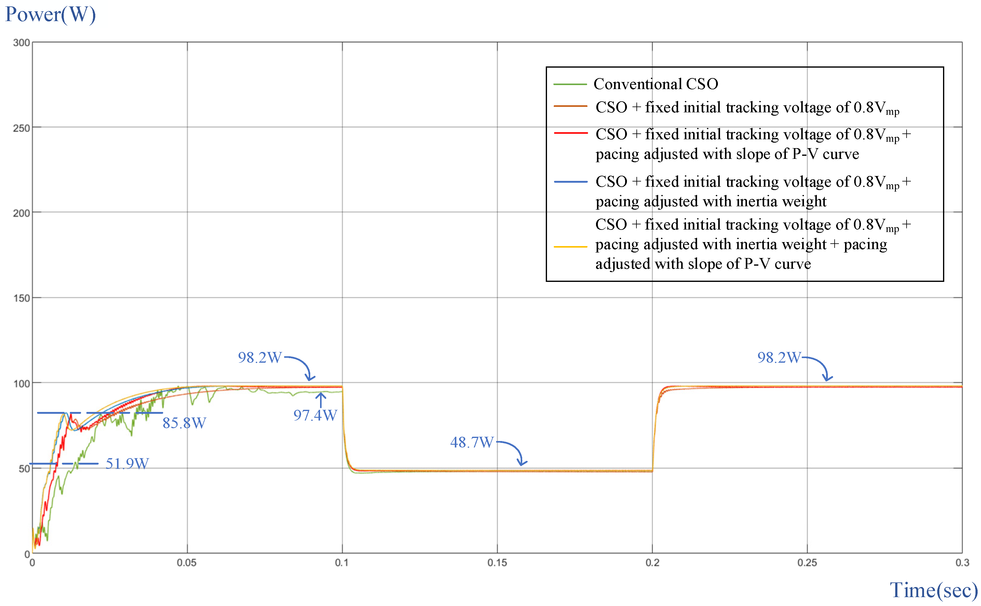
- (5)
- Test of Case 5
- (6)
- Test of Case 6
7. Conclusions
Author Contributions
Funding
Institutional Review Board Statement
Informed Consent Statement
Data Availability Statement
Conflicts of Interest
References
- Akhtar, I.; Kirmani, S.; Jameel, M.; Alam, F. Feasibility Analysis of Solar Technology Implementation in Restructured Power Sector with Reduced Carbon Footprints. IEEE Access 2021, 9, 30306–30320. [Google Scholar] [CrossRef]
- Infield, D.; Freris, L. Renewable Energy in Power Systems; John Wiley & Sons: Hoboken, NJ, USA, 2020; ISBN 1118649931. [Google Scholar]
- Nguyen, T.B.N.; Chao, K.H. Fast Maximum Power Tracking for Photovoltaic Module Array Using Only Voltage and Current Sensors. Sens. Mater. 2023, 35, 2619–2635. [Google Scholar]
- Baba, A.O.; Liu, G.; Chen, X. Classification and Evaluation Review of Maximum Power Point Tracking Methods. Sustain. Futures 2020, 2, 100020. [Google Scholar] [CrossRef]
- Bhukya, L.; Kedika, N.R.; Salkuti, S.R. Enhanced Maximum Power Point Techniques for Solar Photovoltaic System under Uniform Insolation and Partial Shading Conditions: A Review. Algorithms 2022, 15, 365. [Google Scholar] [CrossRef]
- Hanzaei, S.H.; Gorji, S.A.; Ektesabi, M. A Scheme-based Review of MPPT Techniques with Respect to Input Variables Including Solar Irradiance and PV Arrays’ Temperature. IEEE Access 2020, 8, 182229–182239. [Google Scholar] [CrossRef]
- Alrubaie, A.J.; Al-Khaykan, A.; Malik, R.; Talib, S.H.; Mousa, M.I.; Kadhim, A.M. Review on MPPT Techniques in Solar System. In Proceedings of the 2022 8th International Engineering Conference on Sustainable Technology and Development (IEC), Erbil, Iraq, 23–24 February 2022; pp. 123–128. [Google Scholar]
- Díaz Martínez, D.; Trujillo Codorniu, R.; Giral, R.; Vázquez Seisdedos, L. Evaluation of Particle Swarm Optimization Techniques Applied to Maximum Power Point Tracking in Photovoltaic Systems. Int. J. Circuit Theory Appl. 2021, 49, 1849–1867. [Google Scholar] [CrossRef]
- Szemes, P.T.; Melhem, M. Analyzing and Modeling PV with “P&O” MPPT Algorithm by MATLAB/SIMULINK. In Proceedings of the 3rd International Symposium on Small-Scale Intelligent Manufacturing Systems (SIMS), Gjovik, Norway, 10–12 June 2020; pp. 1–6. [Google Scholar]
- Saber, H.; Bendaouad, A.E.; Rahmani, L.; Radjeai, H. A Comparative Study of the FLC, INC and P&O Methods of the MPPT Algorithm for a PV System. In Proceedings of the 19th International Multi-Conference on Systems, Signals & Devices (SSD), Sétif, Algeria, 6–10 May 2022; pp. 2010–2015. [Google Scholar]
- Fan, Z.; Li, S.; Cheng, H.; Liu, L. Perturb and Observe MPPT Algorithm of Photovoltaic System: A Review. In Proceedings of the 33rd Chinese Control and Decision Conference (CCDC), Kunming, China, 22–24 May 2021; pp. 1413–1418. [Google Scholar]
- Zhou, C.G.; Huang, L.; Ling, Z.X.; Cui, Y.B. Research on MPPT Control Strategy of Photovoltaic Cells under Multi-peak. Energy Rep. 2021, 7, 283–292. [Google Scholar] [CrossRef]
- Yang, B.; Zhu, T.; Wang, J.; Shu, H.; Yu, T.; Zhang, X.; Yao, W.; Sun, L. Comprehensive Overview of Maximum Power Point Tracking Algorithms of PV Systems under Partial Shading Condition. J. Clean. Prod. 2020, 268, 121983. [Google Scholar] [CrossRef]
- Javed, S.; Ishaque, K. A Comprehensive Analyses with New Findings of Different PSO Variants for MPPT Problem under Partial Shading. Ain Shams Eng. J. 2022, 13, 101680. [Google Scholar] [CrossRef]
- Huang, Y.P.; Huang, M.Y.; Ye, C.E. A Fusion Firefly Algorithm with Simplified Propagation for Photovoltaic MPPT under Partial Shading Conditions. IEEE Trans. Sust. Energy 2020, 11, 2641–2652. [Google Scholar] [CrossRef]
- Li, C.C.; Sun, C.Y.; Li, S.Q.; Zhang, Y.Y. An Integrated MPPT Control Strategy Using Circle Search-firefly Algorithm (CSFA) for Photovoltaic System. In Proceedings of the 4th International Conference on Smart Power & Internet Energy Systems (SPIES), Beijing, China, 9–12 December 2022; pp. 1945–1949. [Google Scholar]
- Chao, K.H.; Zhang, S.W. An Maximum Power Point Tracker of Photovoltaic Module Arrays Based on Improved Firefly Algorithm. Sustainability 2023, 15, 8550. [Google Scholar] [CrossRef]
- Millah, I.S.; Chang, P.C.; Teshome, D.F.; Subroto, R.K.; Lian, K.L.; Lin, J.-F. An Enhanced Grey Wolf Optimization Algorithm for Photovoltaic Maximum Power Point Tracking Control under Partial Shading Conditions. IEEE Open J. Ind. Electron. Soc. 2022, 3, 392–408. [Google Scholar] [CrossRef]
- Huang, K.H.; Chao, K.H.; Kuo, Y.P.; Chen, H.H. Maximum Power Point Tracking of PV Module Arrays Based on a Modified Gray Wolf Optimization Algorithm. Energies 2023, 16, 4329. [Google Scholar] [CrossRef]
- González, C.; Restrepo, C.; Kouro, S.; Rodriguez, J. MPPT Algorithm Based on Artificial Bee Colony for PV System. IEEE Access 2021, 9, 43121–43133. [Google Scholar] [CrossRef]
- Nagadurga, T.; Narasimham, P.; Vakula, V. Global Maximum Power Point Tracking of Solar Photovoltaic Strings under Partial Shading Conditions Using Cat Swarm Optimization Technique. Sustainability 2021, 13, 11106. [Google Scholar] [CrossRef]
- SunWorld Datasheet. Available online: http://www.ecosolarpanel.com/ecosovhu/products/18569387_0_0_1.html (accessed on 31 October 2022).
- Reddy, D.S. Review on power electronic boost converters. Aust. J. Electr. Electron. Eng. 2021, 18, 127–137. [Google Scholar] [CrossRef]
- Zongo, O. Comparing the Performances of MPPT Techniques for DC-DC Boost Converter in a PV System. Walailak J. Sci. Technol. 2021, 18, 6500. [Google Scholar] [CrossRef]


| Parameter | Value |
|---|---|
| Maximum output power (Pmax) | 20 W |
| Current of maximum output power (Impp) | 1.1 A |
| Voltage of maximum output power (Vmpp) | 18.18 V |
| Short-circuit current (Isc) | 1.15 A |
| Open-circuit voltage (Voc) | 22.32 V |
| Overall dimensions of single module | 395 × 345 × 17 mm |
| Slope Interval of P-V Characteristic Curve | Speed Coefficient (c) in Equation (1) |
|---|---|
| Interval m1: | c = 1.4 |
| Interval m2: | c = 1.3 |
| Interval m3: | c = 1.2 |
| Interval m4: | c = 1.1 |
| Interval m5: | c = 1.0 |
| Interval m6: | c = 1.2 |
| The Inertia Weight (w) in Equation (5) | |
|---|---|
| w = 0.4 | |
| w = 0.35 | |
| w = 0.3 | |
| w = 0.25 | |
| w = 0.2 | |
| w = 0.15 | |
| w = 0.1 |
| Component | Specifications |
|---|---|
| Input capacitor, Cin | , withstand voltage: 400 V |
| Filter capacitance, Cout | , withstand voltage: 450 V |
| Energy storage inductance, Lm | 1.67 mH, withstand voltage: 450 V |
| Fast diode, D (IQVD60E60A1) | Withstand voltage: 600 V, withstand current: 60 A |
| Switch, S (IREP460B) | Withstand voltage: 500 V, withstand current: 20 A |
| Scenario | Peak Numbers on P-V Characteristic Curve | 4-Series, 3-Parallel Shading % |
|---|---|---|
| 1 | Single-peak | (0% shading + 0% shading + 0% shading + 0% shading)// (0% shading + 0% shading + 0% shading + 0% shading)// (0% shading + 0% shading + 0% shading + 0% shading) |
| 2 | Double-peak (MPP at right) | (50% shading + 0% shading + 0% shading + 0% shading)// (0% shading + 0% shading + 0% shading + 0% shading)// (0% shading + 0% shading + 0% shading + 0% shading) |
| 3 | Triple-peak (MPP at right) | (0% shading + 80% shading + 0% shading + 100% shading)// (0% shading + 0% shading + 0% shading + 0% shading)// (0% shading + 0% shading + 0% shading + 0% shading) |
| 4 | Triple-peak (MPP at middle) | (0% shading + 100% shading + 0% shading + 50% shading)// (0% shading + 0% shading + 0% shading + 0% shading)// (0% shading + 0% shading + 0% shading + 0% shading) |
| 5 | Quadruple-peak (MPP at the second peak) | (0% shading + 30% shading + 60% shading + 90% shading)// (0% shading + 30% shading + 60% shading + 90% shading)// (0% shading + 30% shading + 60% shading + 90% shading) |
| 6 | Quadruple-peak (MPP at the third peak) | (30% shading + 50% shading + 80% shading + 0% shading)// (30% shading + 50% shading + 80% shading + 0% shading)// (30% shading + 50% shading + 80% shading + 0% shading) |
| Parameter | Conventional | Modified |
|---|---|---|
| Maximum iteration number (t) | 30 | |
| Random number (r) | [0~1] | |
| Inertia weight (w) | Zero usage w | [0.1~0.4] |
| Speed coefficient (c) | 1.4 | [1.0~1.4] |
| SRD | 0.2% | |
| Case | Number of Peaks on P-V Curve | Tracking Speed | ||||
|---|---|---|---|---|---|---|
| Conventional CSO Algorithm | CSO with Fixed Initial Tracking Voltage | CSO with Fixed Initial Tracking Voltage Combined with Tracking Pace Adjusted with Slope of P-V Curve | CSO with Fixed Initial Tracking Voltage Combined with Tracking Pace Adjusted by Inertia Weight | CSO with Fixed Initial Tracking Voltage Combined with Tacking Pace Adjusted by Slope of P-V Curve and Inertia Weight | ||
| 1 | Single peak | 0.077 s | 0.05 s | 0.048 s | 0.042 s | 0.038 s |
| 2 | Double peak (MPP at right) | 0.061 s | 0.051 s | 0.049 s | 0.003 s | 0.028 s |
| 3 | Triple peak (MPP at right) | 0.082 s | 0.059 s | 0.056 s | 0.04 s | 0.039 s |
| 4 | Triple peak (MPP at middle) | Fail | 0.058 s | 0.055 s | 0.043 s | 0.038 s |
| 5 | Quadruple peak (MPP at second peak) | Fail | 0.037 s | 0.028 s | 0.023 s | 0.02 s |
| 6 | Quadruple peak (MPP at third peak) | Fail | 0.061 s | 0.057 s | 0.056 s | 0.054 s |
| Case | Number of Peaks on P-V Curve | Maximum Oscillation Amplitude | ||||
|---|---|---|---|---|---|---|
| Conventional CSO Algorithm | CSO with Fixed Initial Tracking Voltage | CSO with Fixed Initial Tracking Voltage Combined with Tracking Pace Adjusted with Slope of P-V Curve | CSO with Fixed Initial Tracking Voltage Combined with Tracking Pace Adjusted by Inertia Weight | CSO with Fixed Initial Tracking Voltage Combined with Tacking Pace Adjusted by Slope of P-V Curve and Inertia Weight | ||
| 1 | Single peak | 30 W | 21 W | 11 W | 12 W | 12 W |
| 2 | Double peak (MPP at right) | 18 W | 17 W | 13 W | 14 W | 13 W |
| 3 | Triple peak (MPP at right) | 30 W | 10 W | 9 W | 12 W | 11 W |
| 4 | Triple peak (MPP at middle) | 17 W | 10 W | 8 W | 10 W | 5 W |
| 5 | Quadruple peak (MPP at second peak) | 18 W | 8 W | 10 W | 10 W | 7 W |
| 6 | Quadruple peak (MPP at third peak) | 21 W | 10 W | 12 W | 10 W | 6 W |
Disclaimer/Publisher’s Note: The statements, opinions and data contained in all publications are solely those of the individual author(s) and contributor(s) and not of MDPI and/or the editor(s). MDPI and/or the editor(s) disclaim responsibility for any injury to people or property resulting from any ideas, methods, instructions or products referred to in the content. |
© 2024 by the authors. Licensee MDPI, Basel, Switzerland. This article is an open access article distributed under the terms and conditions of the Creative Commons Attribution (CC BY) license (https://creativecommons.org/licenses/by/4.0/).
Share and Cite
Chao, K.-H.; Nguyen, T.B.-N. Global Maximum Power Point Tracking of a Photovoltaic Module Array Based on Modified Cat Swarm Optimization. Appl. Sci. 2024, 14, 2853. https://doi.org/10.3390/app14072853
Chao K-H, Nguyen TB-N. Global Maximum Power Point Tracking of a Photovoltaic Module Array Based on Modified Cat Swarm Optimization. Applied Sciences. 2024; 14(7):2853. https://doi.org/10.3390/app14072853
Chicago/Turabian StyleChao, Kuei-Hsiang, and Thi Bao-Ngoc Nguyen. 2024. "Global Maximum Power Point Tracking of a Photovoltaic Module Array Based on Modified Cat Swarm Optimization" Applied Sciences 14, no. 7: 2853. https://doi.org/10.3390/app14072853
APA StyleChao, K.-H., & Nguyen, T. B.-N. (2024). Global Maximum Power Point Tracking of a Photovoltaic Module Array Based on Modified Cat Swarm Optimization. Applied Sciences, 14(7), 2853. https://doi.org/10.3390/app14072853