Robust Artificial Intelligence-Aided Multimodal Rail-Obstacle Detection Method by Rail Track Topology Reconstruction

Abstract

Detecting obstacles in the rail track area is crucial for ensuring the safe operation of trains. However, this task presents numerous challenges, including the diverse nature of intrusions, and the complexity of the driving environment. This paper presents a multimodal fusion rail-obstacle detection approach by key points processing and rail track topology reconstruction. The core idea is to leverage the rich semantic information provided by images to design algorithms for reconstructing the topological structure of railway tracks. Additionally, it combines the effective geometric information provided by LiDAR to accurately locate the railway tracks in space and to filter out intrusions within the track area. Experimental results demonstrate that our method outperforms other approaches with a longer effective working distance and superior accuracy. Furthermore, our post-processing method exhibits robustness even under extreme weather conditions.

1. Introduction

Accidents due to the intrusion of foreign objects, such as falling stones into the railway line, often occur during railway transport, seriously endangering the safety of locomotive operation and thus causing serious negative effects [1,2]. Therefore, it is essential to monitor and prevent the obstacles of foreign objects in railway track areas. The current mainstream approaches to rail-obstacle detection can be summarized as visual-based [3,4,5], LiDAR-based [6], and fusion-based [7]; however, these approaches still have many imperfections.

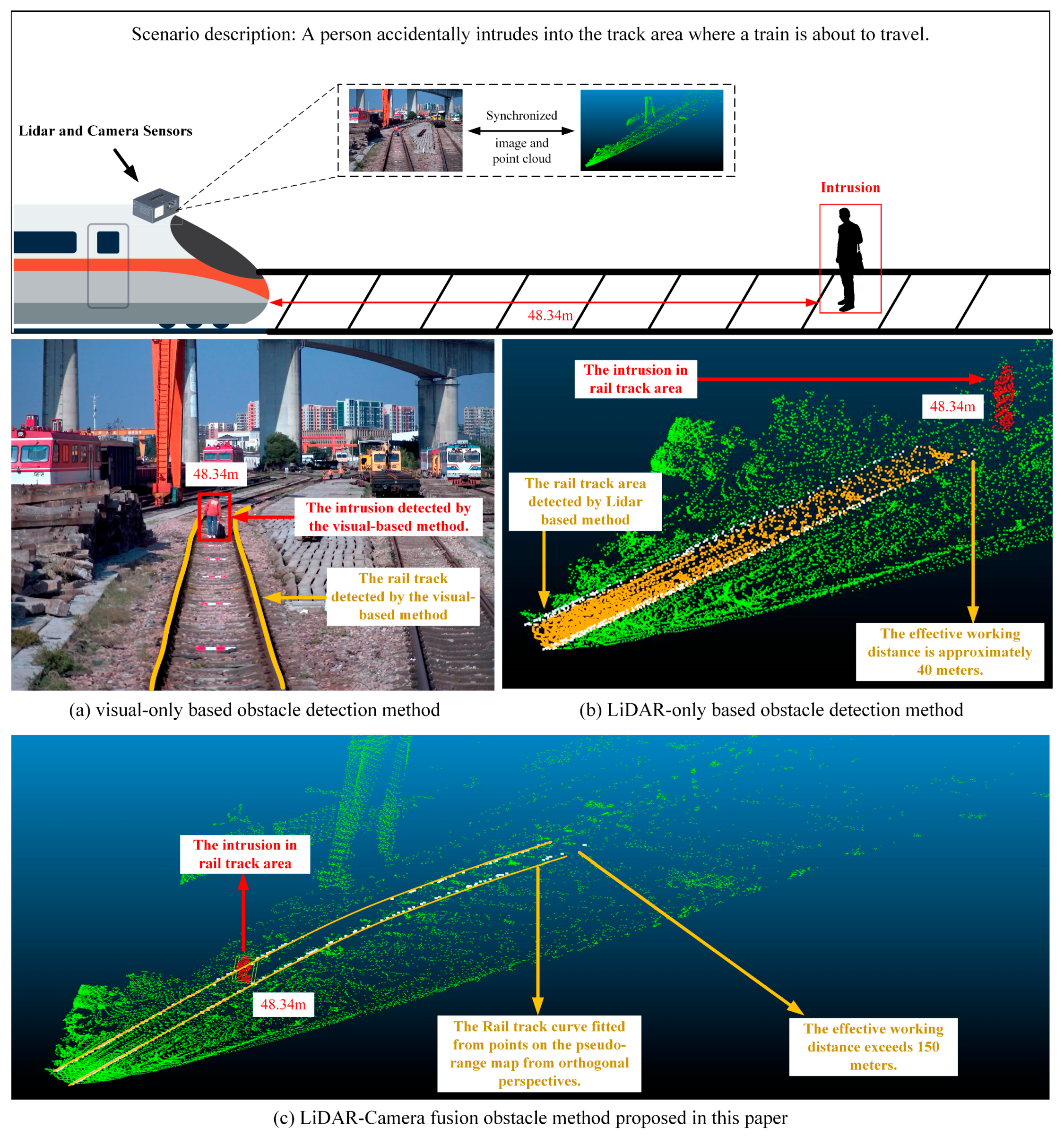
As shown in Figure 1. First, visual-based methods cannot adapt to complex lighting conditions, such as darkness and severe weather. Second, current visual-based methods are poor at identifying small and odd targets such as rocks and tree branches. Furthermore, the visual-based approach cannot provide geometric distance information of intrusions. LiDAR-based [8,9] algorithms are often strongly influenced by the capabilities of the LiDAR and the presence of blind spots or distortions in the LiDAR can significantly affect the performance of the algorithm.

While previous attempts [7,10] have been made to fuse LiDAR and camera data, these methods often rely heavily on the reliability of data, equipment, and neural networks. However, in industrial applications, algorithm designs should be robust. Therefore, we propose a more fault-tolerant and adaptive multimodal fusion scheme.

The core idea of this paper is to leverage the rich semantic features and ideal visual distance provided by a telephoto camera to extract information about the track and track area within the receptive field. Subsequently, utilizing the relative pose relationship between the system, LiDAR, and the camera, the railway tracks are projected into real-world space. Finally, by leveraging the precise spatial information from LiDAR, the presence of intrusions within the track area is determined.

However, in industrial applications, not all modules yield ideal and reliable results. Therefore, the key technical focus of this paper lies in addressing how to determine which feedback information is reliable when the information extracted from the image is not always perfect. Moreover, it aims to reconstruct the track data model using limited but reliable information. Motivated by these challenges, this paper proposes a track topology reconstruction method based on orthogonal projection. Through the establishment of filtering and correction procedures, efforts are made to ensure the reliability of the reconstructed track parameters.

The main contributions of this paper can be summarized as follows:

• Firstly, this paper presents a multimodal rail-obstacle detection, which boasts superior effective working distance and accuracy compared to all existing LiDAR-Camera fusion methods;
• Secondly, we propose a post-processing and reconstruction scheme for neural network-based semantic segmentation results of railway tracks under orthogonal projection. This greatly mitigates system errors caused by errors in semantic segmentation models. Experimental results demonstrate that our post-processing scheme maintains excellent performance stably even in extreme adverse weather and lighting conditions;
• Thirdly, we collect and curate a dataset for railway track reconstruction and intrusion detection. This dataset encompasses various scenarios, including different time periods, road conditions, lighting, and weather, providing robust data support for future research endeavors.

To the best of our knowledge, this paper presents an attempt at implementing a multi-modal rail-obstacle detection algorithm with a focus on railway topology reconstruction. Moreover, this algorithm demonstrates a certain level of compatibility with adverse weather conditions and lighting environments.

2. Related Work

Rail track area intrusion detection is a popular research topic, and there are three main technical approaches: visual-based [3], LiDAR-based [6], and fusion-based approaches [7]. References [11,12] provide comprehensive summaries of existing methods.

2.1. Visual Based Method

Most existing visual-based methods [13,14,15,16] detect the bounding boxes of intrusion targets in images by means of supervised deep learning-based target detection [17,18]. For example, Refs. [19,20,21] explore image-based methods using high-definition imagery. Pan et al. [22] designed a branching network to perform semantic segmentation of the image inside and outside the tracked area and then determine whether the detected target is within the tracked area. Such approaches can solve the track intrusion detection problem more accurately but it is worth noting that the visual-based approach cannot obtain the distance of the intruder. However, such methods lack the definition of the detection object inside or outside the rail track [23]. First, visual-based methods cannot adapt to complex lighting conditions, such as darkness and severe weather. Second, current visual-based methods are poor at identifying small and odd targets such as rocks and tree branches. Furthermore, the visual-based approach cannot provide geometric distance information of intrusions.

2.2. LiDAR Based Method

The point cloud output from the LiDAR provides feedback on the distance of the object and reflectivity information. Using prior calibration information and the characteristics of the track presented in the point cloud, it is also possible to determine the tracked area and identify intruders within the tracked area [19,24,25]. However, methods based on LiDAR input are more dependent on the quality of the point cloud. In situations where the point cloud quality is suboptimal, the performance of such methodologies experiences a pronounced decline.

2.3. Fusion Based Method

LiDAR-Camera fusion-based approaches have been widely used in the field of autonomous driving [26,27,28,29]. In the field of rail track area intrusion detection, existing work also has high requirements for the density and resolution of point clouds [30,31,32,33]. Wang et al. [7] conducted a reprojection of point clouds onto an image and utilized the image semantic segmentation output to identify point clouds within the track area. These identified point clouds were then fitted to a reference surface, and any points above the reference surface within the rail track area were classified as intrusion objects. However, this method relies on the quality of image segmentation results and the quality of the point cloud, which is often difficult to qualify in practice, so a more robust method needs to be devised. Inspired by the above work, we propose a fusion-based method to detect intrusion objects in rail track areas.

3. Approach

According to prior information, there are two main geometrical characteristics of railway tracks:

Characteristic 1. The left rail line and the right rail line of the same rail track are parallel.

Characteristic 2. In medium distances (e.g., within 1 km), the slope of the track changes sufficiently slowly that it can be abstractly assumed that the tracks within the working distance of our method lie on a single plane [34].

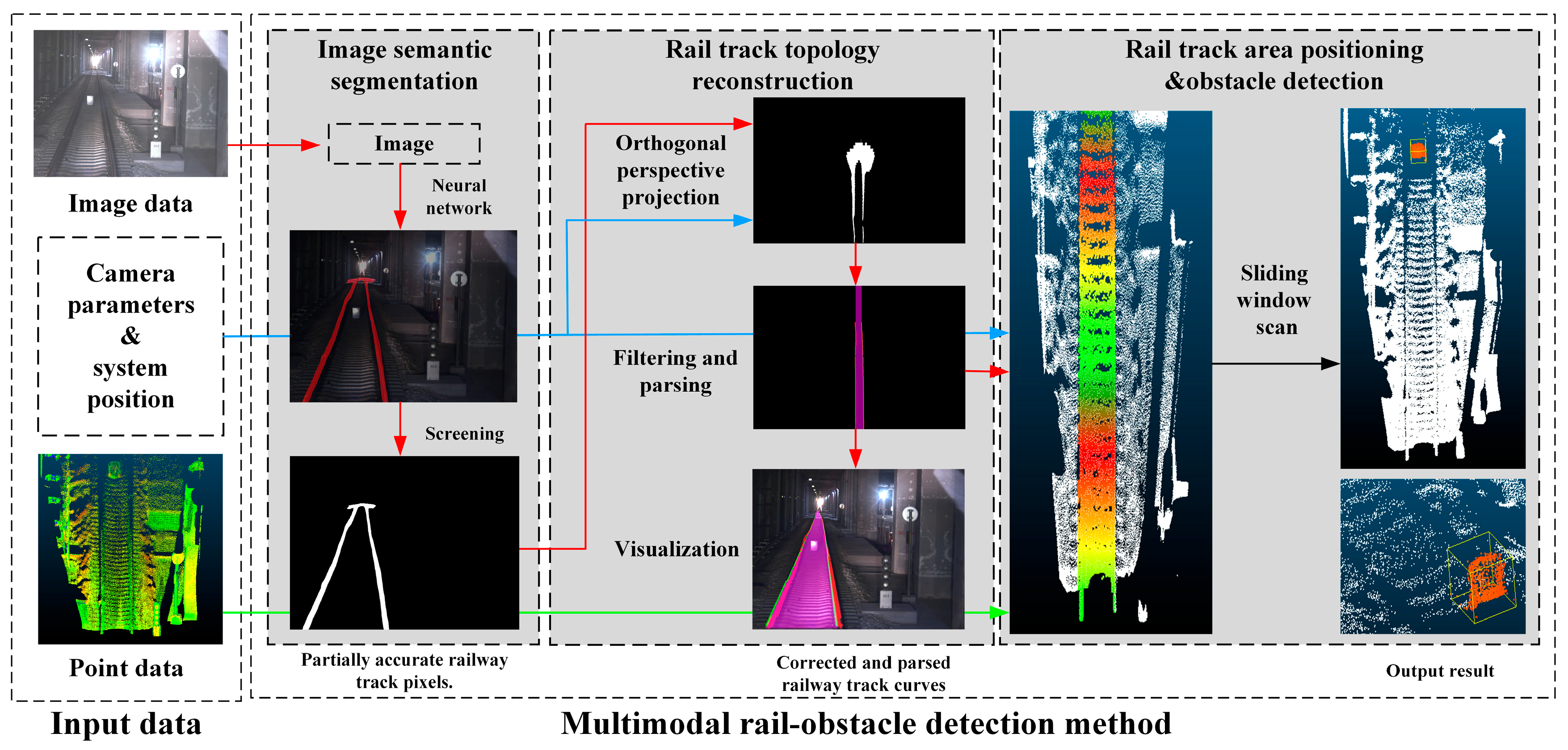
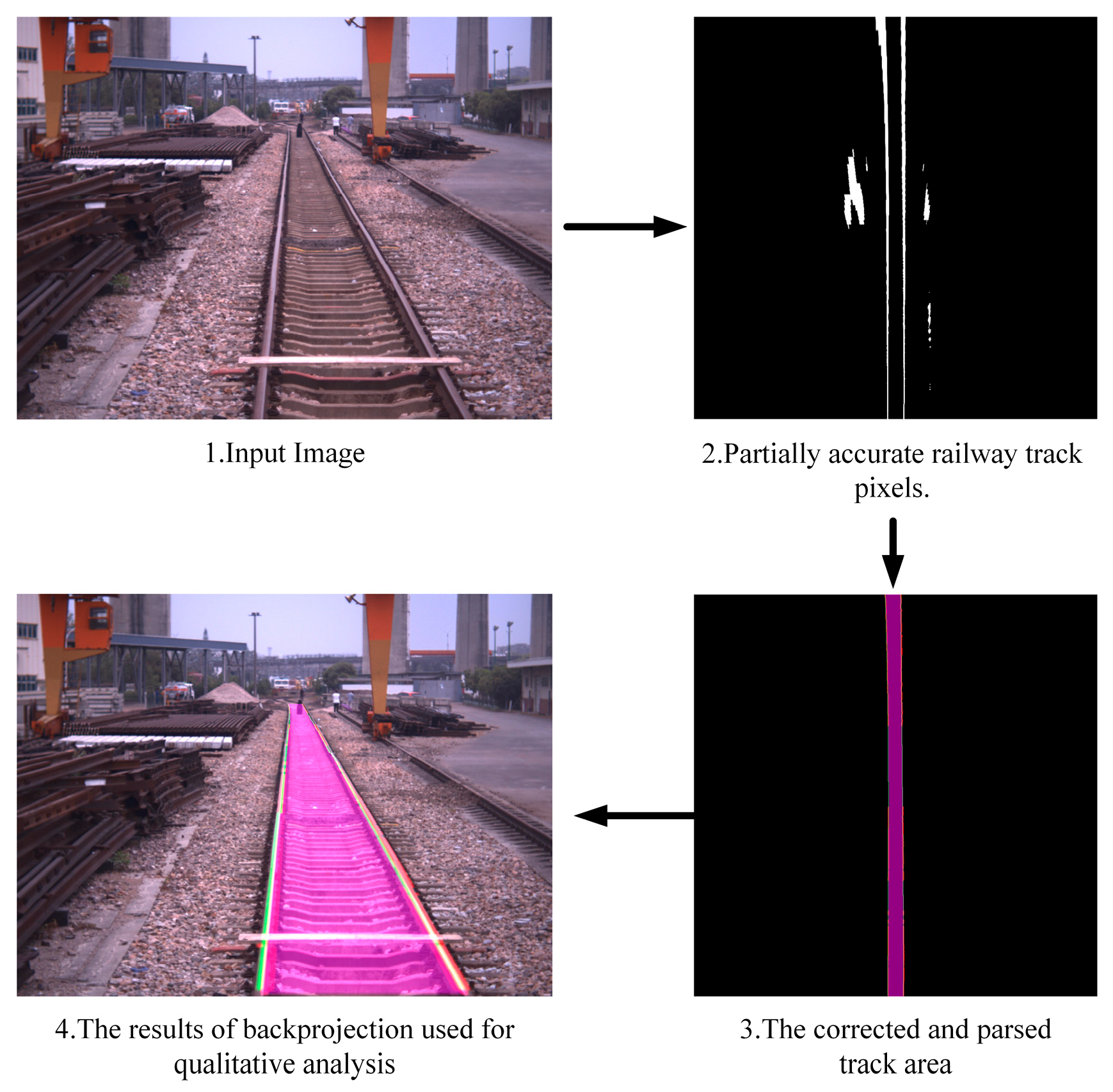
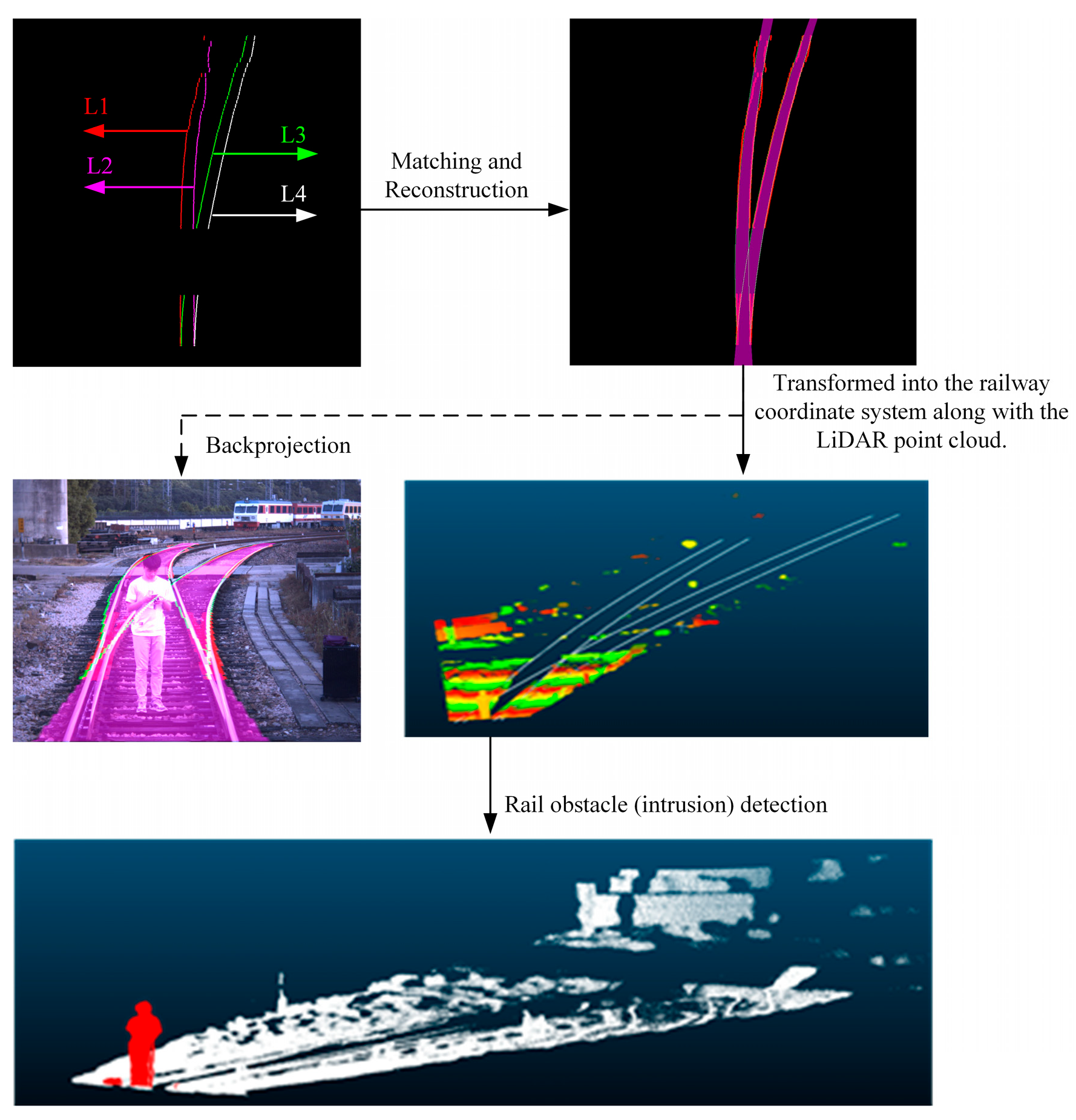
Based on the aforementioned analysis, this paper introduces a track area intrusion detection method using rail track topology analysis. The proposed approach is divided into three main stages: image semantic segmentation, rail track topology reconstruction, and rail track area intrusion detection. The overall flowchart is depicted in Figure 2. The overall process of the algorithm is briefly summarized as follows: first, perform semantic segmentation on the image and obtain the Bird’s Eye View (BEV) view of track pixels through orthogonal projection, referred to as the “orthogonal map”. Then, use track reconstruction algorithms to filter and correct track pixels and reconstruct the topological representation of the track using these pixels. Finally, project the track and LiDAR point cloud into a predefined rail coordinate system and use intrusion detection algorithms to identify intrusions in the track area.

3.1. Image Semantic Segmentation

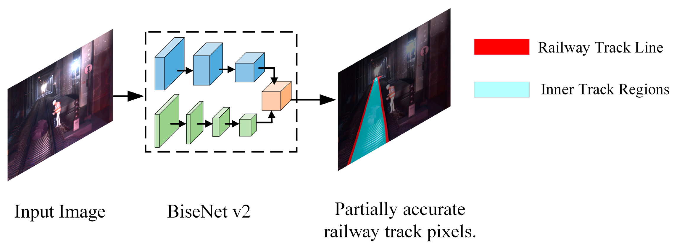
As shown in Figure 3, a lightweight neural network, BisenetV2 [35], is trained supervised using a publicly dataset Railsem19 [36]. This training endeavor aims to yield an image input and a corresponding neural network output delineating three distinct categories: railway track line, inner track regions, and the image background.

It is worth noting that the result of the segmentation is discrete at this point. We can currently only obtain a classification of each pixel in the image but have no information about the geometry of the rail track. In addition, there are some incorrect outcomes for semantic segmentation, so further correction and parsing of the semantic segmentation results using geometric information are needed.

3.2. Rail Track Topology Reconstruction

3.2.1. Coordinate System Setup

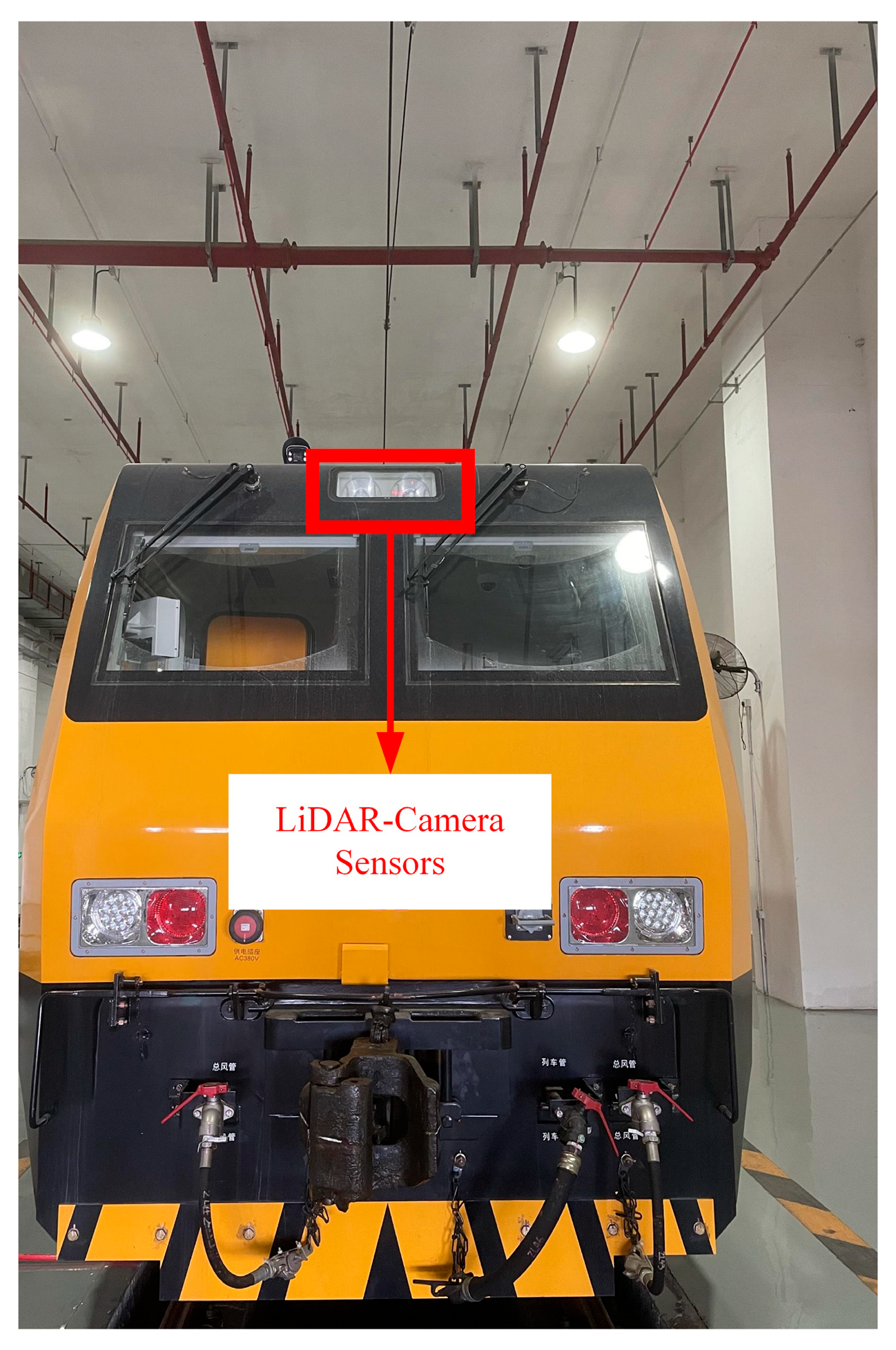
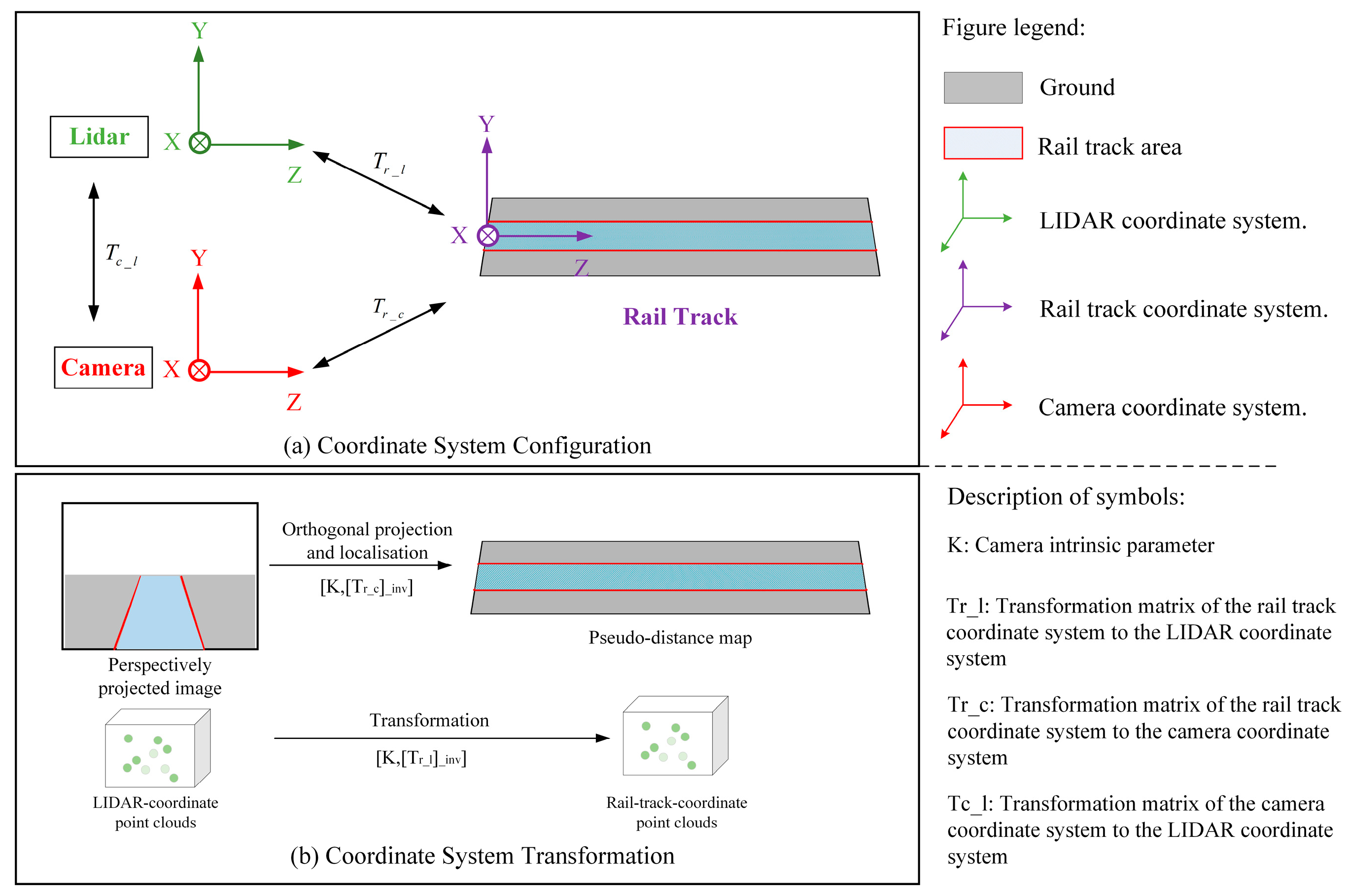
Our train-mounted equipment is installed as shown in Figure 4. Our algorithm implementation requires one LiDAR and one telephoto camera, both mounted on the top of the train’s locomotive. It is worth noting that the positions of the LiDAR and camera are parallel to the ground. However, the images captured by the camera exhibit a perspective projection relationship with the real world. We propose a method to transform perspective-projected images into orthogonal projection and then perform post-processing under orthogonal projection.

Under orthogonal projection, a pair of rail lines are parallel and their pixel dimensions are proportional to the actual distance. We therefore use a homography transformation [34] to convert the image of the perspective projection into an orthogonal projection and use the camera parameters and poses to localize the orthogonal image, as shown in Figure 5b.

As shown in Figure 5a, we set the midpoint of the track directly below the front of the train as the origin of the rail coordinate system, the direction of travel of the train as the z-axis, the axis perpendicular to the rail plane and facing upwards as the y-axis, and the direction of the x-axis pointing to the left of the z-axis. The camera and LiDAR coordinate systems are set up similarly. The normal vector of the image plane is aligned with the z-axis, facing outwards, while the vector pointing upwards is aligned with the y-axis. The x-axis is positioned to the left of the z-axis.

The transformation relationship between the camera coordinate system and the rail coordinate system is shown in Equation (1), where $Z_c$ is the depth of the object point to the image plane, $K$ is the camera intrinsic parameters, and $T_{r\_c}$ is the extrinsic parameters of the camera relative to the rail coordinate system. In our system, the pixel coordinate of the image is represented by $u$ and $v$ where u represents the horizontal pixels, while v represents the vertical pixels. The railroad track coordinate is represented by $X_r$, $Y_r$, and $Z_r$.

$$Z_c\left[\begin{array}{c}u\\ v\end{array}\right]=K{T}_{r\_c}\left[\begin{array}{c}{X}_r\\ Y_r\\ Z_r\end{array}\right],Y_r=0$$

(1)

Based on Characteristic 2, the points in the rail track area all have zero Y-values in the rail coordinate system and a linear system of equations can be created with known parameters to calculate the point coordinates in the rail coordinate system for each pixel in the camera coordinate system.

$$\left[\begin{array}{c}u\\ v\\ 1\end{array}\right]=M\left[\begin{array}{c}{X}_r\\ 0^T\\ Z_r\end{array}\right],M=\left[\begin{array}{cc}R& t\\ 0^T& 1\end{array}\right]$$

(2)

$$\left[\begin{array}{c}{X}_r\\ 0\\ Z_r\\ 1\end{array}\right]=S\left[\begin{array}{c}{u}_0\\ v_0\\ 1\\ 1\end{array}\right]$$

(3)

This transformation process is shown by Equation (2), where M is the transformation matrix from camera to rail coordinates [37,38]. The orthogonal projection can be considered as a scaling and rotation of the points in the rail track coordinate system, this process can be represented by (3), where S is the transformation matrix of the two coordinate systems and $u_0$ and $v_0$ are the pixel points of the orthogonal image coordinate system. Similarly, the LiDAR point cloud is projected in the rail coordinate system using a similar approach. The subsequent detection algorithm and the corresponding output results are based on the rail coordinate system as the reference coordinate system.

3.2.2. Railway Track Correction and Clustering

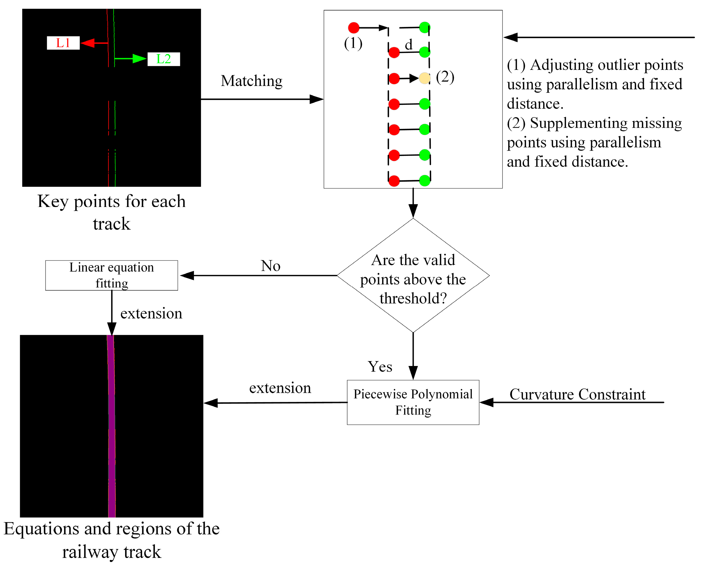
The semantic segmentation results after orthogonal projection are first screened initially to retain the valid key points. After the momentum tracking method proposed in this paper, the key points in the orthogonal map are connected as rail track lines and, based on the fitted curve, the railway line points can be clustered. In this paper, the distribution of a single railway track into left and right tracks is defined as L1 and L2. If there are branching points, additional branches are defined such as L3, L4, and so forth.

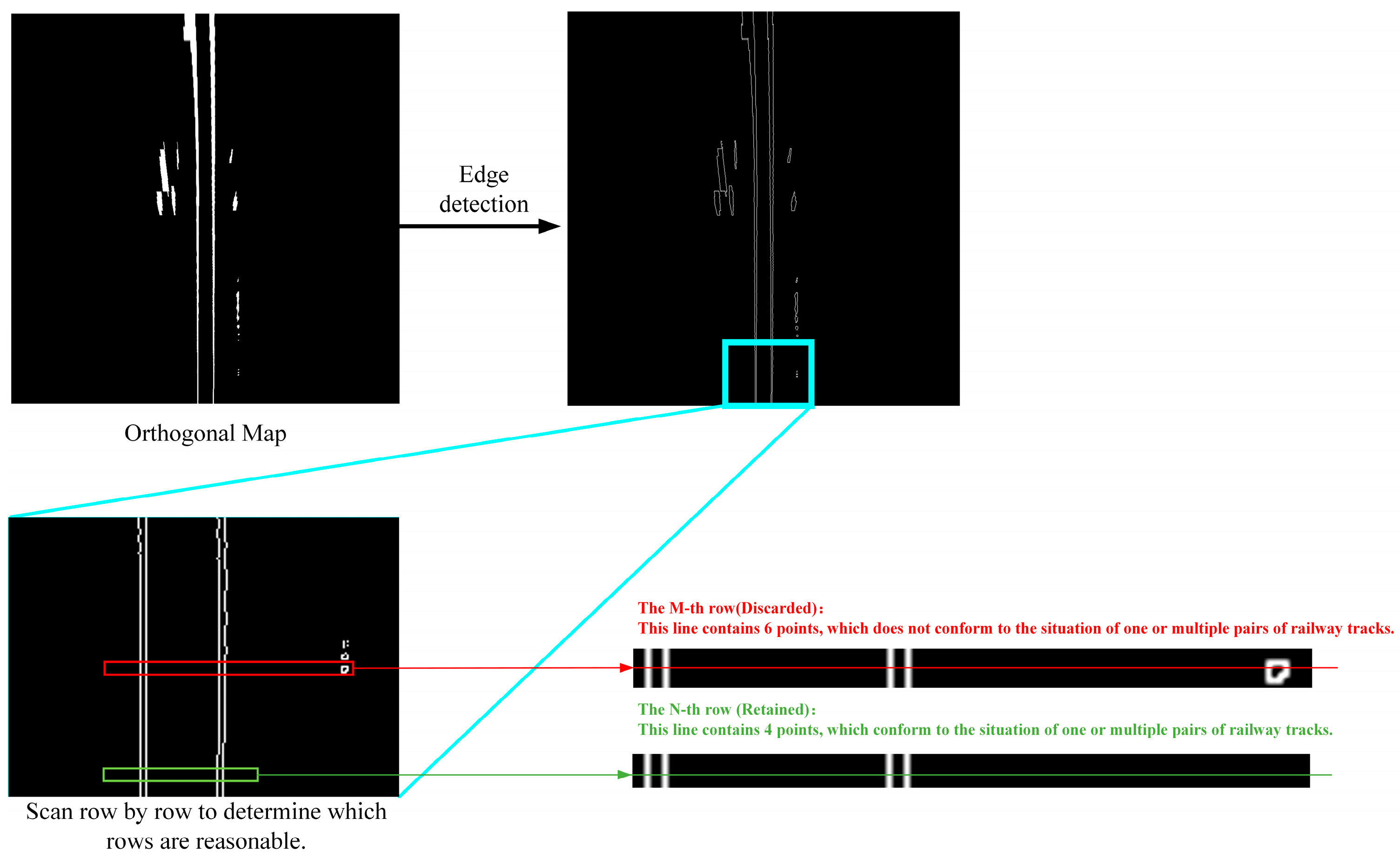
As shown in Figure 6, the orthogonal map result is first edge-detected [39] to find the left and right boundaries of the railway track lines. Specifically, the orthogonal image should be denoted as $O(u,v)$. Gaussian smoothing should be performed on it as shown in Equation (4), resulting in the smoothed image $G(u,v)$.

$$G(u,v)=\frac{1}{2\mathit{\pi }{\mathit{\sigma }}^2}{e}^{-\frac{u^2+v^2}{2{\mathit{\sigma }}^2}}\times O(u,v)$$

(4)

On the smoothed image, compute the gradients in the horizontal and vertical directions using the Sobel operator. The formula for computing the gradient is Equations (5) and (6) as follows:

$$G_u=O(u+1,v)-O(u-1,v)$$

(5)

$$G_v=O(u,v+1)-O(u,v-1)$$

(6)

where $G_u$ and $G_v$ are the gradients in the horizontal and vertical directions, respectively. Then, compute the magnitude and direction of the gradient using Equations (7) and (8):

$$M(u,v)=\sqrt{G_u^2+G_v^2}$$

(7)

$$\mathit{\theta }(u,v)=\arctan (\frac{G_x}{G_y})$$

(8)

where $M(u,v)$ is the magnitude of the gradient and $\mathit{\theta }(u,v)$ is the direction of the gradient. For the gradient magnitude image, retain pixels with local maximum gradients and suppress non-maximum values. Then, determine which edge pixels are true edges by setting high and low thresholds. Pixels above the high threshold are considered strong edge pixels, while pixels connected to strong edge pixels but below the low threshold are considered weak edge pixels. By performing edge tracking, convert weak edge pixels to strong edge pixels to obtain the final edge image [40].

Based on Characteristic 2, a set of railway tracks can be conceptualized as two parallel lines. In other words, within a reasonable distance, a pair of railway tracks are parallel and coplanar. Therefore, when the semantic map is projected onto the bird’s eye view (BEV) perspective, a true pair of railway tracks should have four edge points. This holds true even in the presence of switches where the number of edge points remains a multiple of 4. Based on the analysis above, we can conduct a row-by-row search on orthographic images to identify the correct railway track points. When scanning boundary points row by row, a rail line pair can be found with two boundary points in a single row. Therefore, in one row of the orthographic image, a pair of railway tracks should have four edge points. The initial coarse screening process involves removing boundary points from the railway track that are not equal to four or multiples of four within the same row.

Through this approach, we retain valid track points for each row in the orthographic image. For rows deemed invalid, we discard all track points within that row. While this may result in a certain degree of information loss, subsequent techniques such as curve fitting compensate for this loss. Empirical evidence suggests that the lost information does not significantly affect the experimental results.

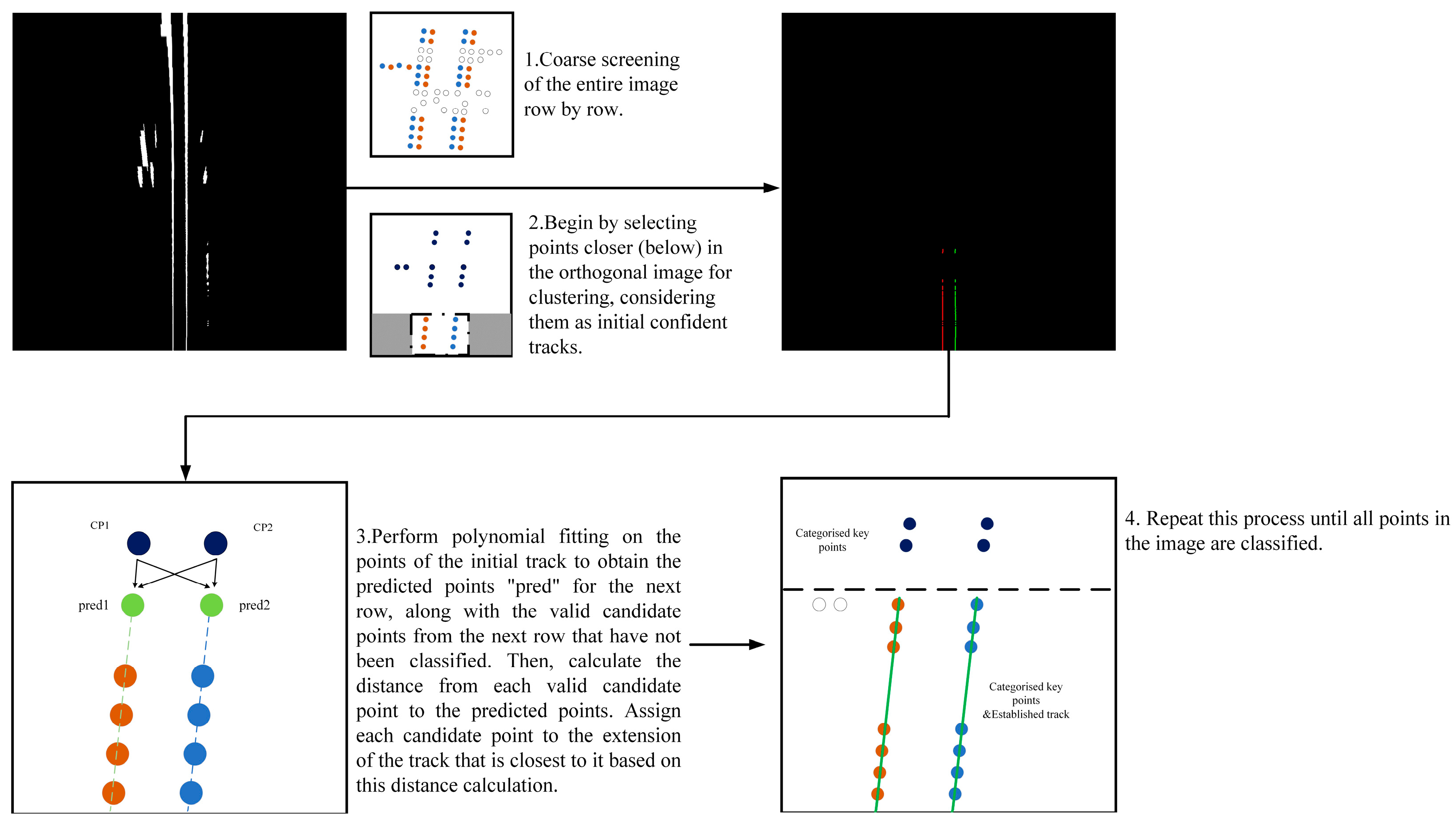
The initial coarse screening process involves removing boundary points from the railway track that are not equal to four or multiples of four within the same row. Figure 7 illustrates this screening process. Then, it selects the inner boundary points of the railway track as the candidate points for fitting. Following the coarse screening, points in the central region of the lower part of the orthogonal image are chosen as initial points. These points are theoretically positioned directly beneath the train and represent the area the train is about to traverse. The majority of these initial points are utilized to ascertain the number of tracks. For instance, if the majority of initial points in each row is four, it can be assumed that the train does not pass the switch ahead of it. When the train passes a switch, the majority of the initial points are eight. The key points of the first 100 rows of the graph are chosen as the initial points in this paper, as shown in Figure 7.

Since it is not known which switch the train will be heading to, the track area for both teams of tracks needs to be calculated. Once the number of tracks has been determined using the initial points, a polynomial fit to the inner boundary of each pair of tracks is selected as an abstraction of the initial rail track alignment.

After generating prediction points for the next row, the method calculates the distance between each candidate point and the corresponding prediction point. If the minimum distance falls below the threshold, the candidate point is categorized as belonging to that track; otherwise, it is disregarded. This process is outlined in Algorithm 1 and Figure 7.

Algorithm 1: Railway Points Selection and Reconstruction

Input: p(u, v): Pixel set of railway tracks under orthogonal map $H_{init}$: Number of rows for preset initial confidence points Output: $L_j^{3d}$: Point set of railway track lines, where i is the number of rail lines.

for i = 1 to $H_{init}$ do   (1) $P_i$ = Iterative filter key points in row i   (2) $P_{i\_v}=\{p\in P_i|\left|p\mathrm{mod}4\right|=0\}$ end //Determine the initial confidence region’s location on a single rail line or a diverging track based on the filtering results. (3) if (singleRailLine) { allocateToL1toL2 ($P_{i\_v}[:100,0]$,$P_{i\_v}[:100,1]$) } else if (divergingTrack) allocateToL1ToL4 ($P_{i\_v}[:100,0]$,$P_{i\_v}[:100,1]$,$P_{i\_v}[:100,2]$,$P_{i\_v}[:100,3]$) } for i to the num of rails do   for j = 1 to $H_{init}$ do     //Least squares fitting     (4) $F(u_{Lij})=\underset{{\mathit{\theta }}_{0,}{\mathit{\theta }}_1,{\mathit{\theta }}_2}{\min }{\displaystyle \sum _{idx=1}^j(v_{Lij}-({\mathit{\theta }}_0+}{\mathit{\theta }}_1{u}_{Lij}+{\mathit{\theta }}_2{u}_{Lij}^2))$     //Predict the key points of the next row based on the existing polynomial and add the maximum likelihood point to the existing rail line key points set.     (5) $L_i$= update_clusters ($L_i$,$P_{j+1}$)     //Update the parametric equations for each rail lines.     (6) $F(u_{Lij})=\underset{{\mathit{\theta }}_{0,}{\mathit{\theta }}_1,{\mathit{\theta }}_2}{\min }{\displaystyle \sum _{idx=1}^{j+1}(v_{Li(j+1)}-({\mathit{\theta }}_0+}{\mathit{\theta }}_1{u}_{Li(j+1)}+{\mathit{\theta }}_2{u}_{Li(j+1)}^2))$ end (7)//Convert pixel coordinates to 3D coordinates based on the geometric information from the orthogonal range map. $L_j^{3d}$= projection ($L_j^{2d}$) Return $L_j^{3d}$

3.2.3. Fitting of the Track Area

Firstly, for each railway track, we divide them into 10 equal parts based on the perception range from nearest to farthest. Under normal circumstances, each part is fitted with a quadratic polynomial curve, as shown in equation 9.

$$L_{ji}(z_j)=a_i{z}_j^2+b_i{z}_j+c_i(0\le j<10)$$

(9)

where $L_j$ represents the equation of the j-th track, i denotes the i-th segment, a, b, and c are the parameters to be fitted, and z is the independent variable distance.

We artificially impose some constraints on the formula shown in Equation (9). Firstly, we match each pair of tracks and utilize the parallelism between the two tracks, as well as the fixed distance between them, to constrain the parameter fitting. Specifically, after matching a pair of railway tracks, based on prior information that the left and right tracks are parallel and separated by a fixed distance d, we can utilize this characteristic to correct any outliers in the tracks and fill in missing points accordingly. Furthermore, based on prior Characteristic 1 and Characteristic 2, we limit the size of $a_i$ as a constraint on curvature. The process of railway topological reconstruction is shown in Figure 8.

Additionally, we devise a contingency plan to handle extreme cases. We set a threshold n and if the number of key points for a particular pair of tracks is less than the threshold n, we abandon the segmented polynomial fitting for that track and instead opt for linear fitting. Figure 9 illustrates the qualitative results of the aforementioned process. Once the interpretation of the railway track is obtained, we set a fixed distance. When the distance of the detected key points is less than the preset distance, we extend the track appropriately based on the first and last segments of the segmented curve. The curve parameter fitting methods all use the least squares method [41].

3.3. Rail Track Intrusion Detection

Further analysis of rail track intrusion by aligning the tracked area of the orthogonal map with the LiDAR point clouds in the track coordinate system. Analysis of the point cloud within the rail track area along the distance axis, i.e., the z-axis, on a distance-by-distance basis in meters. In other words, after determining the track area in space according to Equation (10), as shown, a sliding window is set along the z-axis direction, measured in meters. Then, the region is inspected meter by meter to detect any intrusion.

$$R_{area}=\{(X,Y,Z)\in R^3|L_{right}(Z)<X<L_{left}(Z)\}$$

(10)

During the rail-obstacle search process, we set two primary criteria for intrusion detection. One criterion is height: if there is a cluster of points higher than the track plane, it is suspected to be an intrusion. Additionally, to enhance robustness and mitigate the impact of adverse weather (raindrops, snowflakes, etc.) and noise from the equipment itself, we incorporate point cloud density as a judgment criterion. Theoretically, the point cloud density of intrusions decreases with distance but it differs significantly from noise.

Whereas the height constraint is a constant value H = 0.4 m, the constraint on point cloud density, through experimentation, is found to be ideally modeled as a quadratic decay. This is illustrated as $\Theta =N-a^{*}{z}^2$ where N is set to 420 and a is set to 0.01. The rail-obstacle detection process is shown in Algorithm 2. For the intrusion detection process, Figure 10 illustrates an example using a turnout as a reference.

Algorithm 2: Intrusion detection

Input: P(x,y,z): point cloud in rail track area Length: the longest distance for reconstructing rail tracks H: Height Criteria $\Theta$: Density Criteria Output: $I\in R^{1\times Z}$: Rail area intrusion labels (in meters on the Z axis)

For i = 1 to Length do //$R_{area}$ refers to the track area currently locked by the sliding window. $R_{area}$ = Slidewindow(Z = i) if $R_{area}$ = None then I (Z = i) = 0 else if $Y_{\max }$ = maximum value of Y in $R_{area}$ $\mathit{\rho }(z)$ = point cloud density in $R_{area}$ if $\mathit{\rho }(z)$ > $\Theta$ and $Y_{\max }$ > H then I (Z = i) = 1 else I (Z = i) = 0 Return I

4. Dataset

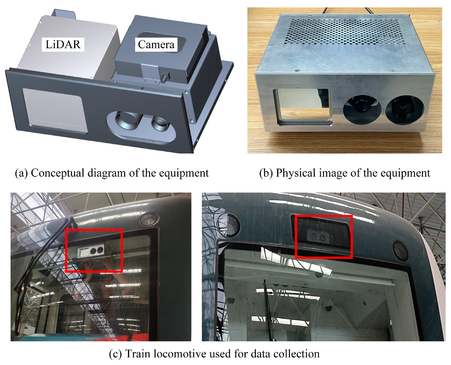
In this paper, there are two datasets. One is the open-source image dataset RailSem19 [36], which is used for training the semantic segmentation neural network. The other dataset is the tracked area intrusion detection dataset that we collected using a synchronized Alvium G5-1240 camera with a focal length of 25 mm and a LiDAR to capture image-point cloud pairs. The original resolution of this camera is 3036 × 4024 pixels. However, for training and inference using deep learning networks, we resized the images to 512 × 1024 pixels. Our camera is a color camera and for nighttime driving, illumination from the train’s headlight was relied upon. There are two models of LiDAR: Titan-M1-R LiDAR from Neuvition and Livox-Tele15. The repetition rate of the solid-state LiDAR is chosen as 2 KHz as a frame and the resolution of the image is 3036 × 4024, as shown in Figure 11.

Figure 11a depicts the data acquisition device we designed, which includes a pair of parallel LiDARs and cameras. Their optical centers are aligned parallelly. Figure 11b depicts the physical setup of our data collection, while Figure 11c shows two different train heads. We used these two trains to collect data on different routes.

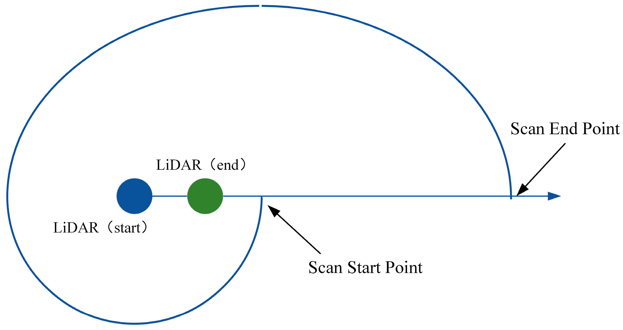
Furthermore, as illustrated in Figure 12, to address the errors caused by vehicle motion during data collection, we employed a uniform acceleration model for motion calibration of the point cloud. Assuming the initial pose of the LiDAR scan is $p_i^1$, we assumed that during the scanning process, the vehicle can be considered to undergo uniform acceleration (or uniform motion). Assuming that the train moves without any rigid body rotation during operation, only undergoing displacement transformation, we can calculate the displacement of each point relative $p_i^t$ to $p_i^1$ at each moment through velocity integration. Then, by applying a translation transformation, we can eliminate the motion errors. This is shown in Equations (11) and (12).

$$\Delta d={\displaystyle \underset{0}{\overset{t}{\int }}(v_0+at)dt=v_{0}t+\frac{1}{2}}a{t}^2$$

(11)

$$p_i^1=p_i^t-\Delta d$$

(12)

We manually calibrated the parameters required for the experiment and collected a large-scale dataset of simulated train intrusion on different subway and train routes. Where $v_0$ is the current initial velocity, a is the acceleration and t is the time interval of the point cloud relative to the initial scan point. We collected a total of 11 routes, encompassing various scenes, weather conditions, and lighting conditions. There are a total of 7547 pairs of synchronized image-point cloud data.

Partial images from the dataset are shown in Figure 13. For quantitative analysis, we selected four representative routes for manual annotation. We annotated the track areas in the images and whether there were intrusions in the point clouds. These four datasets include scenarios such as switchbacks, tunnels, curves, and straight sections. Additionally, they include common intrusions in railway tracks such as pedestrians of various sizes, backpacks, suitcases, and umbrellas. To validate the accuracy of railway track reconstruction, we deliberately included some objects outside the track but close to it, referred to as “negative hard samples”.

Table 1. Statistics of the proposed dataset.

Name	Pedestrian	Umbrella	Luggage	Package	Negative Hard
numbers	156	144	144	60	253

represents the content of the dataset. The dataset was collected for four scenarios: tunnel, switchback, curves, and straightaways. The dataset comprises 156 instances of pedestrian intrusion scenes, 144 instances of umbrella intrusion scenes, 144 instances of luggage (medium-sized objects) intrusion scenes, and 60 instances of parcel (small-sized objects) intrusion scenes. Additionally, there are 253 instances of negative hard sample scenes, where objects are close to the track but do not intrude.

Figure 14 depicts the statistical information of intruding objects contained in the annotated dataset from the overall dataset. The horizontal axis represents the index of intruding objects, while the vertical axis represents the distance of intruding objects. Our evaluation metrics are mainly accuracy, recall, precision, and F1 metrics, according to [42]. Based on the above actual situation, we choose the recall rate, which is more sensitive to missed alarm situations, as the main evaluation metric; the F1 score as the secondary evaluation metric; and other evaluation metrics as auxiliary evaluation metrics.

$$precision=\frac{Tp}{Tp+Fp}$$

(13)

$$recall=\frac{Tp}{Tp+Fn}$$

(14)

$$accuracy=\frac{Tp+Tn}{Tp+Tn+Fp+Fn}$$

(15)

$$F1=\frac{2\times Tp}{2\times Tp+Fp+Fn}$$

(16)

where Tp (true positive) is the number of samples correctly predicted as positive, Fp (false positive) is the number of samples incorrectly predicted as positive, Fn (false negative) is the number of positive samples incorrectly predicted as negative, and Tn (true negative) is the number of samples correctly predicted as negative.

Regarding the method for handling rail-obstacle detection, our approach and some state-of-the-art methods (e.g., Wang et al. [7]) employ a semantic segmentation submodule for image preprocessing/processing. We train this submodule using the RailSem19 dataset, utilizing all 8500 annotated images from RailSem19 as the training set. Additionally, we utilize 757 images collected and annotated by ourselves as the test set in the semantic segmentation task.

However, it is important to note that the RailSem19 dataset is specific to semantic segmentation tasks and provides ground truth only for semantic segmentation tasks, which are unrelated to our research on “rail-obstacle detection”. The dataset is merely used to train certain submodules of our methods that involve image semantic segmentation. Therefore, RailSem19 images cannot serve as evaluation data for our task.

For the task addressed in this paper, as there are currently no publicly available datasets, we have collected our own dataset and manually annotated a portion of it as a contribution to this study. In the “Dataset” Section, we provide detailed information about the collection process and the results of our annotations.

Since our workload and innovations do not involve deep learning, the original parts of our algorithm do not pertain to model training. Therefore, we have not designated a training set; instead, we use all the point-cloud-image pairs from the track intrusion dataset as the test set.

In summary, all experimental results are based on the dataset we collected and annotated ourselves. The RailSem19 dataset is only utilized to provide necessary supervision for specific submodules and cannot serve as any evaluation basis. We have added detailed explanations of the dataset in the updated manuscript to ensure clarity in our presentation.

5. Experiments

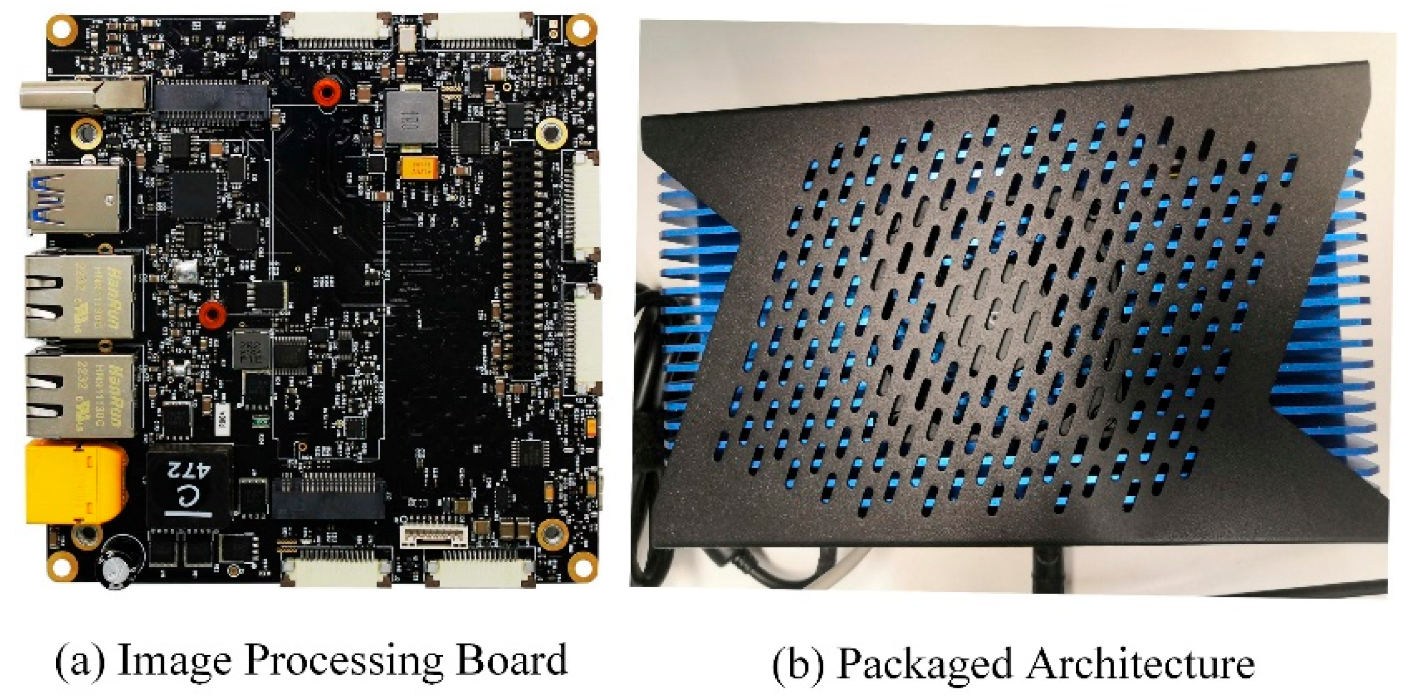
As shown in Figure 15, we implemented our algorithm as an engineering application using Nvidia’s Jetson AGX Xavier development board. In the development board, we encapsulate our algorithm using the ROS architecture. We set up three parallel nodes: one node subscribes to synchronized LiDAR point cloud and camera image data from the device, the second node handles image segmentation and post-processing, and the third node is responsible for segmenting the images and parsing the projected track from the LiDAR point cloud. It then performs track intrusion detection tasks and outputs the detection results.

5.1. Comparison with Existing Methods

We select two rail track instruction detection techniques—the ‘LiDAR-based method [43]’ and the ‘fusion method [7]’—to compare with our approach. Inspired by [43,44,45,46], the ‘LiDAR-based method’ uses prior information to segment the rail track areas from the point cloud and calculates the intrusion. In

Table 2. Overall results of different methods on the proposed dataset.

Method	Rec.	F1	Pre.	Acc.	Time
LiDAR Only [43,45,46]	0.401	0.354	0.452	0.990	0.147 s
Wang et al. [7]	0.892	0.418	0.374	0.971	3.162 s
Ours	0.982	0.909	0.900	0.999	0.270 s

,

Table 3. Performance of the rail-obstacle approach at different distances.

Distance	Method	Rec.	F1	Pre.	Acc.
<40 m	LiDAR only [43,45,46]	0.872	0.311	0.437	0.972
	Wang et al. [7]	0.987	0.576	0.565	0.939
	Ours	0.994	0.986	0.991	1.000
<60 m	LiDAR only [43,45,46]	\	\	\	\
	Wang et al. [7]	0.982	0.526	0.487	0.949
	Ours	0.989	0.972	0.974	1.000
<100 m	LiDAR only [43,45,46]	\	\	\	\
	Wang et al. [7]	0.923	0.397	0.363	0.944
	Ours	0.985	0.910	0.900	0.997
<160 m	LiDAR only [43,45,46]	\	\	\	\
	Wang et al. [7]	0.899	0.418	0.372	0.964
	Ours	0.982	0.909	0.900	0.998
<200 m	LiDAR only [43,45,46]	\	\	\	\
	Wang et al. [7]	0.892	0.418	0.374	0.971
	Ours	0.982	0.909	0.900	1.000

and

Table 4. Performance of the rail-obstacle approach in different scenarios.

Distance	Method	Rec.	F1	Pre.	Acc.
Switchback	LiDAR only [43,45,46]	0.372	0.381	0.077	0.990
	Wang et al. [7]	0.770	0.249	0.141	0.936
	Ours	1.000	0.956	0.938	1.000
Tunnel	LiDAR only [43,45,46]	0.524	0.352	0.108	0.992
	Wang et al. [7]	0.732	0.660	0.892	0.997
	Ours	0.955	0.947	0.963	0.999
Curve	LiDAR only [43,45,46]	0.934	0.514	0.938	1.000
	Wang et al. [7]	0.443	0.667	0.443	0.981
	Ours	0.635	1.000	0.675	0.996
Straightaway	LiDAR only [43,45,46]	\	\	\	\
	Wang et al. [7]	0.667	0.276	0.206	0.948
	Ours	0.975	0.975	0.987	1.000

of the updated manuscript, we selected the best results from [43,45,46] as the outcomes of the “LiDAR-based” technique and compared them with other methods. However, we found that different methods led to some variations in results but there was no significant improvement or deterioration. This is because the performance of this type of technique depends on the characteristics of the LiDAR equipment. As shown in Figure 1, when the input point cloud data contain few track points and are close in distance, even with ground truth used for prediction, the algorithm cannot achieve a long effective working distance. We reproduce the method proposed by [7] as a ‘fusion method’; where the track is segmented, the point cloud is reprojected onto the image, and then a rail track area surface is fitted using the point cloud. If there is a point cloud in the track area that appears above the fitted surface, then the area is considered to be intruded. In the diagrams of this paper, we refer to the ‘fusion method’ as ‘Wang et.al’ to distinguish it from our work.

Table 2 presents the comparative results of overall metrics for the methods mentioned in the paper. From the results in Table 2, we can compare and conclude that the performance of methods based solely on LiDAR is mediocre. According to this method, the recall rate is 40.1%, the precision rate is 45.2%, and the F1 score is only 35.4%. This is because such methods heavily rely on the quality of equipment and input data. Even though these methods can effectively handle existing point clouds, they struggle to perform well when the point cloud data itself lacks meaningful information. On the other hand, Wang et al.’s fusion method showed a significant improvement in recall, reaching 89.2%. However, there is no significant improvement in precision and F1 score, which are only 41.8% and 37.4%, respectively. This is because their method is based on spatial plane fitting of trajectory regions obtained from semantic segmentation. However, the results of semantic segmentation are not always reliable and even slight deviations can lead to discrepancies in the fitted plane angles. Although they extended the effective working distance of the algorithm, the deviation in plane fitting led to missed detections, resulting in no significant improvement in precision and F1 score. Our method, on the other hand, focuses on improving the effective working distance and robustness of sub-modules. As a result, our false detection rate and missed detection rate are relatively low. In terms of performance metrics, our method exhibits excellent accuracy, recall, and F1 score, reaching 98.2%, 90.9%, and 90.0%, respectively. This is nearly a 200% improvement compared to methods solely based on LiDAR. Since most intrusion detection algorithms are sensitive to missed detections, for safety reasons, the penalty for missed detections far outweighs that for false alarms. Therefore, all algorithms achieve an objective level of accuracy within their effective working distances. It is worth noting that our algorithm has been optimized to achieve a processing time of 0.27 s/frame. Although this is not as fast as the 0.147 s/frame of methods based solely on LiDAR, our algorithm exhibits significantly higher accuracy than such methods. In contrast, Wang et al.’s method requires approximately 3.162 s to complete processing, with the majority of the time consumed by point cloud projection and plane fitting operations.

In summary, it can be observed that our proposed method demonstrates superiority across all evaluation metrics. This is because our method combines LiDAR and a camera for track reconstruction, resulting in a much greater effective working distance compared to other methods. Moreover, based on our post-processing approach, the algorithm’s results are not overly reliant on the performance of devices such as LiDAR and cameras. Furthermore, our method achieves an inference time of 0.270 s per frame, which is superior to the method proposed by Wang et al.

The experimental results presented in Table 3 further illustrate the performance metrics of different methods at various working distances. At a distance of 40 m, we observed that methods solely based on LiDAR achieved passable accuracy, with a rate of 87.2%. However, due to the lack of crucial input data, LiDAR-based methods are unable to effectively predict longer distances. Therefore, both Wang et al.’s method and our method utilize cameras effectively to extend the effective working distance. Wang’s method, employing plane fitting, exhibits increasing errors with distance, resulting in a recall rate of 98.7% at 40 m but dropping to 89.2% at around 200 m. In contrast, our method shows no significant decrease, maintaining a recall rate of 98.2% even at 200 m.

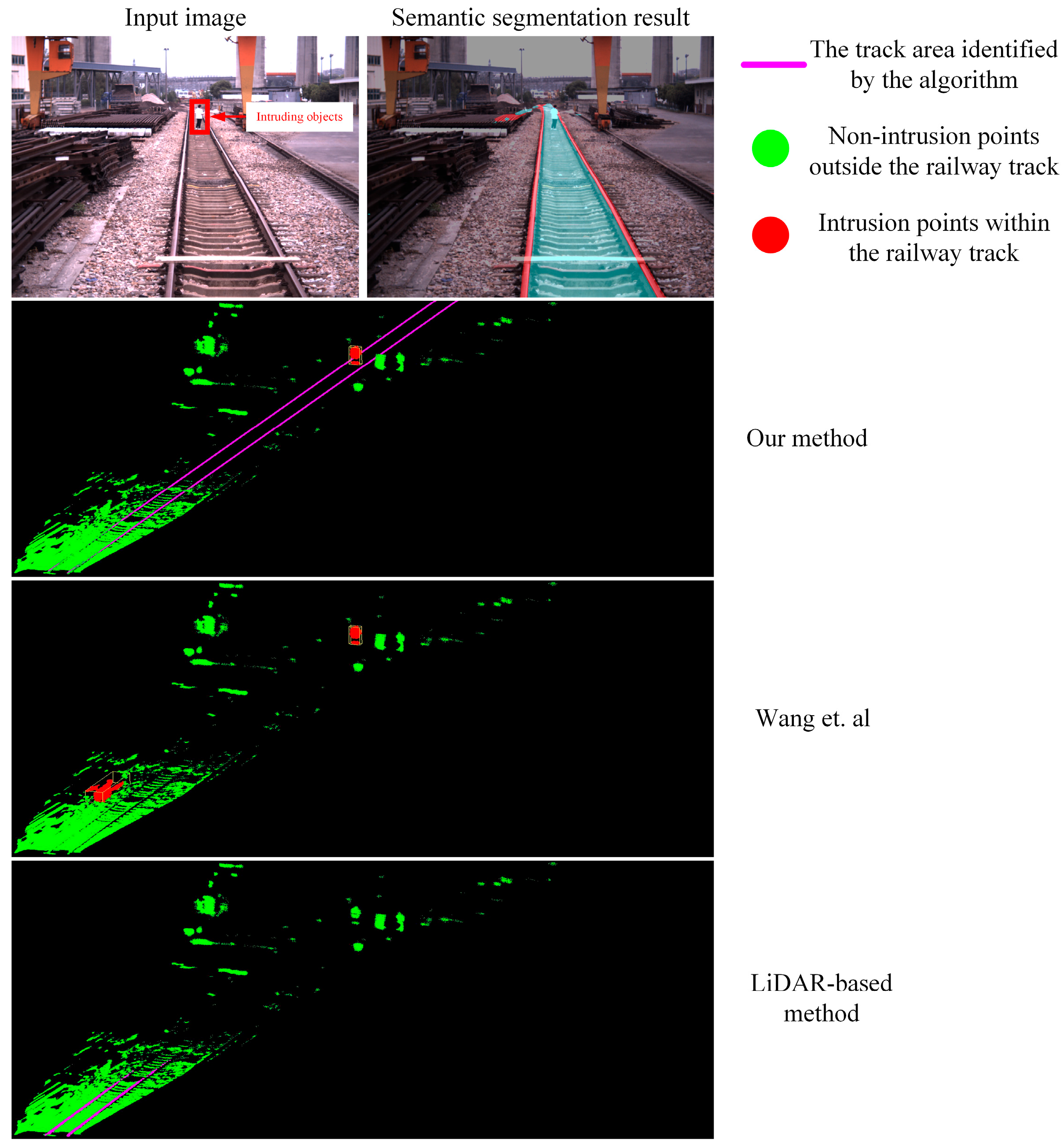
Compared to other fusion methods, our proposed method exhibits better overall performance and does not suffer from significant accuracy degradation at different distances. As shown in Figure 15 and Figure 16, we present two typical data cases to illustrate the superiority of our approach.

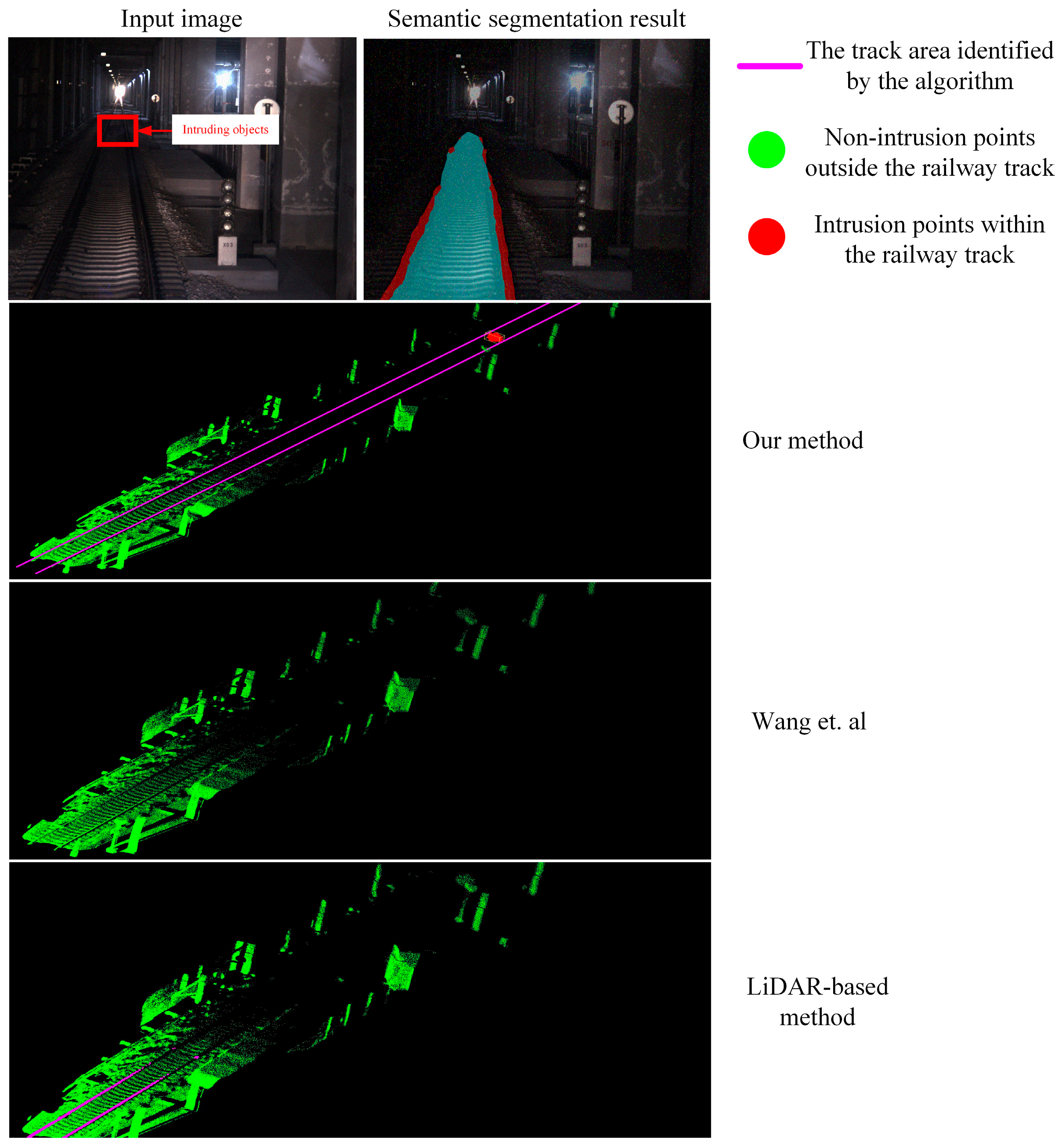
As shown in Figure 16, Wang et al.’s method fails to obtain correct track area point clouds, while the radar-based method cannot acquire sufficient valid points. Our method, however, analyzes and reconstructs the track in space based on limited points, resulting in the correct track area. In Figure 17, the intruding object is located far from the device and there are some errors in the semantic segmentation results, incorrectly identifying the steel bars on the left as the track and considering part of it as the track area. Solely relying on LiDAR-based methods, due to insufficient valid points, cannot identify the position of the track area at a distance and therefore cannot determine the intrusion situation in the distance. As for Wang’s method, since there is no post-processing of the semantic segmentation results, errors in the semantic segmentation results often directly affect the final result of the algorithm. Meanwhile, our method effectively reconstructs the correct track area and accurately identifies the intrusion object.

Table 4 illustrates the comparison of our algorithm’s results with other methods in different scenarios in the dataset we proposed. The conclusions drawn from Table 4 further support our argument. Our method demonstrates superior performance at railway switches, with a recall rate of 100% and an accuracy rate of 93.8%, outperforming other methods. This is attributed to the challenges faced by radar-based methods in calculating complex railroads and the inclination of fitted planes due to semantic segmentation errors in Wang et al.’s method. Our approach, based on track reconstruction, maximally adapts to complex scenarios. However, the performance on curved tracks is slightly inferior to methods based on LiDAR. Our method achieves a recall rate of 63.5%, while LiDAR-based methods achieve 93.4%. This is because the data collection time for this scenario is mostly during the night, when cameras cannot obtain effective semantic information, whereas lidar can scan the surrounding scene clearly. Nevertheless, overall, our method still demonstrates significant superiority.

Our method performs well in switchback, tunnels, and straight sections. In the straight section scenario, intrusion objects are relatively far away, making LiDAR-only methods ineffective. In the curve scenario, LiDAR-only methods benefit from their accurate geometric information, resulting in good performance in the precision metric.

5.2. Ablation Study

In addition to comparing with other methods, we also conducted experiments to evaluate the effectiveness of the main modules of our proposed method. Firstly, we performed ablation experiments to assess the effectiveness of the railway track reconstruction method.

We manually annotated the images in our dataset and then compared the tracks reconstructed by the track reconstruction method with the tracks projected back onto the images. We conducted pixel-wise comparisons between the projected tracks and the manually annotated ground truth. We used two metrics, MPA (mean pixel accuracy) and MIoU (mean intersection over union), for quantitative analysis, as shown in Equations (17) and (18) [47,48].

$$MIoU=\frac{1}{n+1}{\displaystyle \sum _{i=0}^n\frac{T{p}_i}{T{p}_i+F{p}_i+F{n}_i}}$$

(17)

$$MPA=\frac{1}{n+1}{\displaystyle \sum _{i=0}^n\frac{T{p}_i}{T{p}_i+F{n}_i}}$$

(18)

We manually annotated the images in our dataset and then compared the tracks reconstructed by the track reconstruction method with the tracks projected back onto the images. We conducted pixel-wise comparisons between the projected tracks and the manually annotated ground truth. We used two metrics, MPA (mean pixel accuracy) and MIoU (mean intersection over union), for quantitative analysis. In the experiments shown in

Table 5. Results of the ablation experiments for rail reconstruction curves.

Reconstruction Methods	MIoU	MPA
Semantic segmentation	0.705	0.782
Polynomial Fitting	0.795	0.887
Piecewise Polynomial Fitting	0.803	0.891
Piecewise Polynomial Fitting + Extreme Case Constraints + Extension	0.858	0.917

, “n” represents the category, representing only two categories: “track” and “non-track”. The meanings of “Tp”, “Fp”, and “Fn” are the same as in Equations (13)–(16).

In accordance with Equations (17) and (18), the experimental results are shown in Table 5. “Semantic Segmentation” refers to the semantic segmentation results without any further processing. “Polynomial Fitting” represents fitting the entire track into a single polynomial curve. “Piecewise Polynomial Fitting” involves dividing the entire track into 10 segments and fitting each segment with a polynomial curve. “Extreme Case Constraints” indicates the utilization of prior information about the tracks to constrain the curves. “Extension” denotes the appropriate extension of the track when the distance between detected key points is insufficient.

From Table 5, it can be seen that our post-processing methods effectively corrected the results of the semantic segmentation network. Furthermore, we obtained the equations representing the railway tracks as well as their projections in space, delineating the track zones.

Table 6. Results of ablation experiments for the rail-obstacle scanning method.

Height Criteria	Density Criteria	Rec.	F1	Pre.	Acc.
>0.4 m	\	0.985	0.510	0.403	0.987
>0.4 m	$>100 \mathrm{pts}/{\mathrm{m}}^3$	0.958	0.676	0.588	0.994
>0.4 m	$>300 \mathrm{pts}/{\mathrm{m}}^3$	0.865	0.698	0.652	0.995
>0.4 m	$>N-a^{*}{z}^2 \mathrm{pts}/{\mathrm{m}}^3$	0.982	0.913	0.906	0.999
>0.3 m	$>N-a^{*}{z}^2 \mathrm{pts}/{\mathrm{m}}^3$	0.986	0.807	0.773	0.997
>0.5 m	$>N-a^{*}{z}^2 \mathrm{pts}/{\mathrm{m}}^3$	0.895	0.842	0.916	0.998
>0.6 m	$>N-a^{*}{z}^2 \mathrm{pts}/{\mathrm{m}}^3$	0.824	0.780	0.915	0.998

illustrates the impact of different intrusion criteria for trackside objects on the experimental results. “Height Criteria” represents the minimum threshold for intrusion detection when scanning with a sliding window. From the experimental results in Table 6, it is found that setting the height threshold too low can increase false alarms, thereby affecting precision-related metrics, while setting it too high can lead to missed detections, negatively impacting recall-related metrics. Meanwhile, “Density Criteria” represents the threshold for the minimum point cloud density required to detect intrusion within a fixed window. We compared three settings: a fixed threshold of 100 points, 300 points, and the density threshold mentioned in the paper, which decays with distance. Based on the experimental results in Table 6, we believe that selecting a fixed height threshold of 0.4 m and a density threshold function that decays with distance is a reasonable choice.

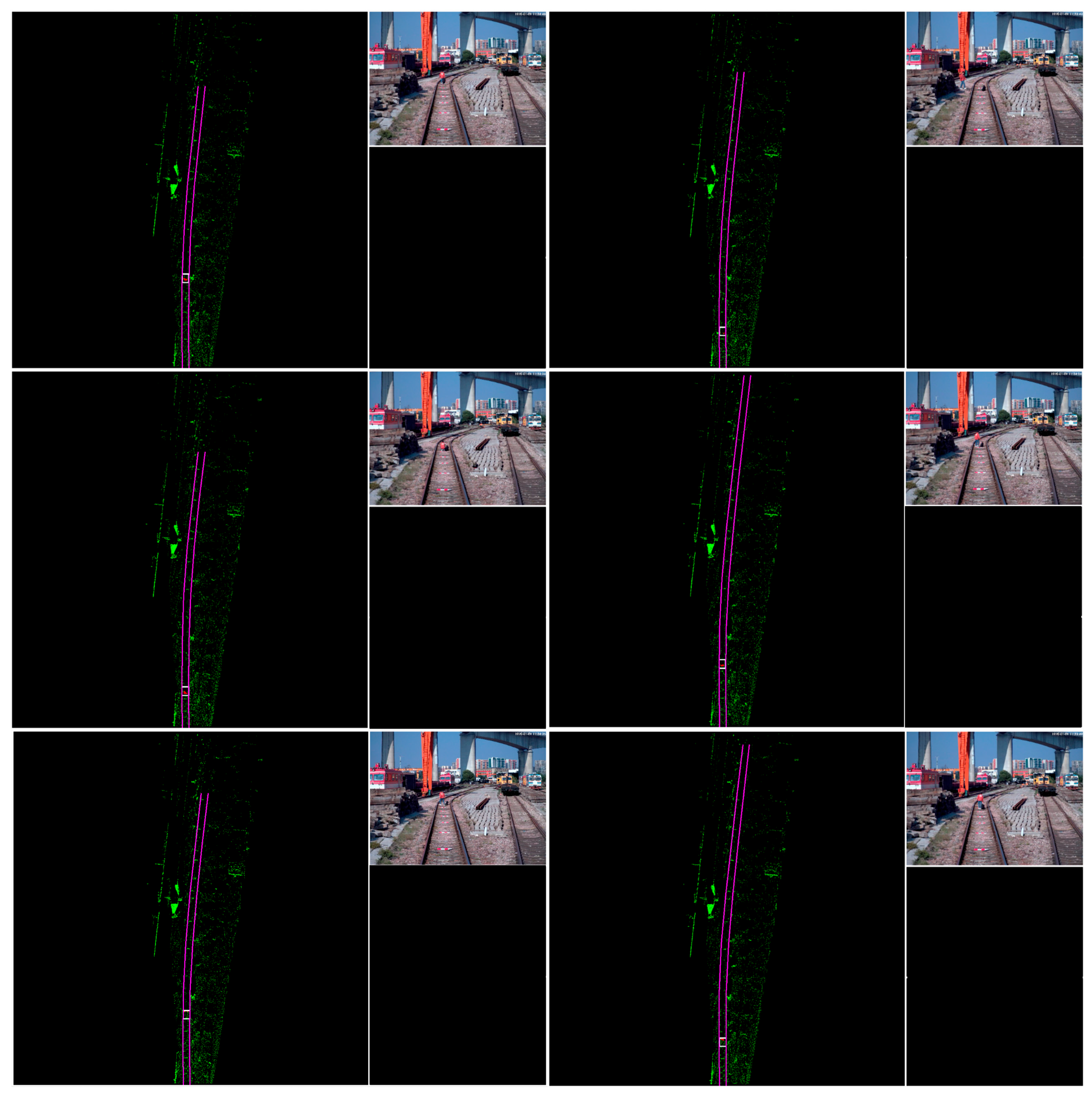
We conducted a quantitative analysis of the algorithm’s resource utilization, the results of which are presented in Figure 18. It depicts the qualitative analysis results with a bird’s-eye view perspective. It is evident that the tracks reconstructed by our algorithm align well with the real tracks and that intrusions within the track are accurately and promptly detected.

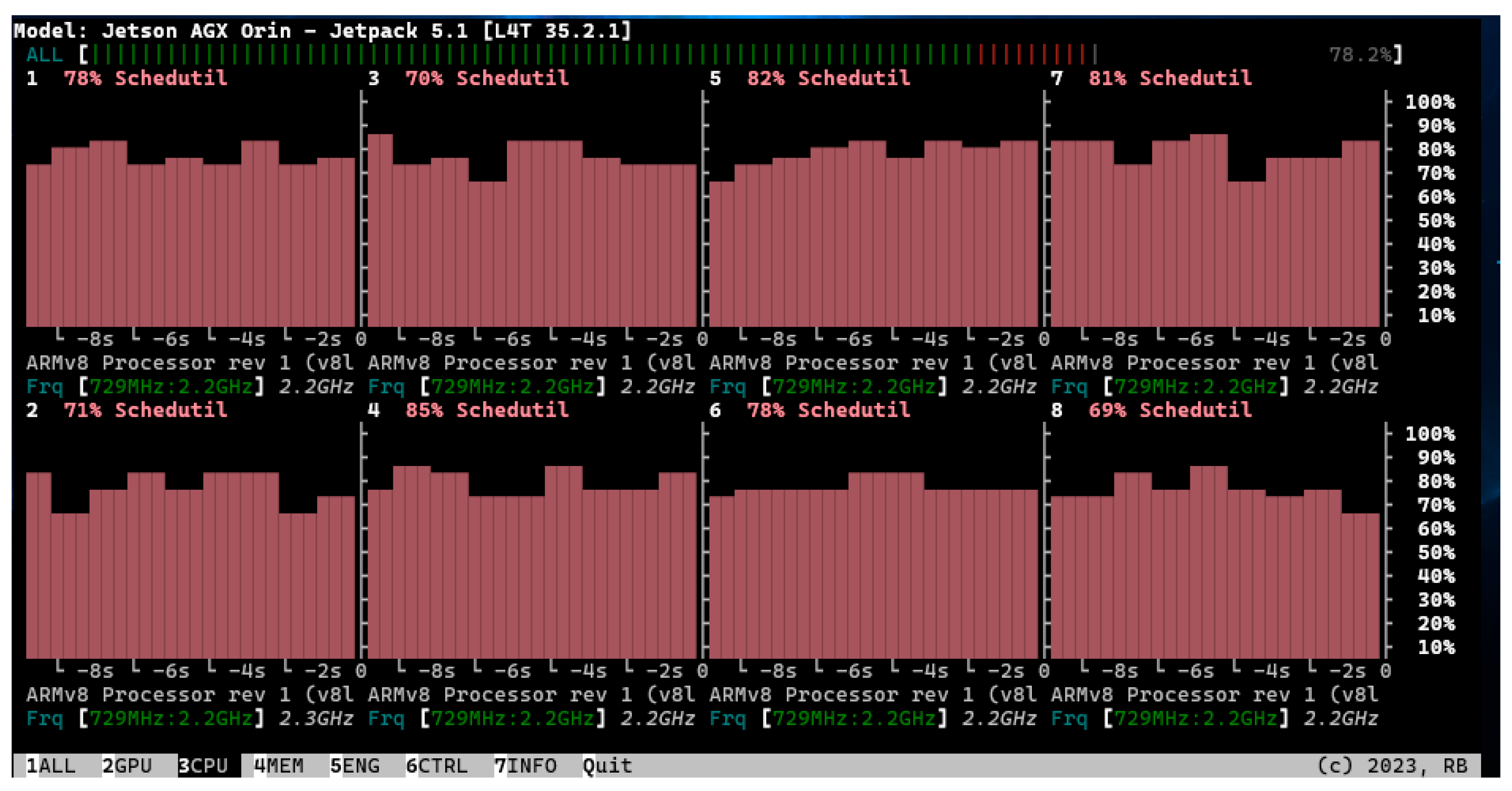
In addition to the semantic segmentation model (which requires negligible time and computational resources), all our algorithms run on the CPU of the development board. We utilize multiple threads to simultaneously process input data from data nodes, perform algorithm computations, and produce output data for output nodes. The overall resource utilization accounts for approximately 80% of the entire development board’s capacity, as shown in Figure 19. However, the runtime per frame reaches 0.27 s, which is sufficient to meet the detection requirements during train operation.

5.3. Discussion

In this chapter, we conducted experiments using our self-collected and annotated dataset. As shown in Table 2, our method significantly outperforms the ones based solely on LiDAR and even Wang et al.’s method in terms of quantitative results. We can explain this phenomenon based on the results in Table 3. Firstly, LiDAR-based methods lack point cloud data for the track, so even if the algorithm’s accuracy is high, it cannot provide effective information to judge distant targets. Secondly, Wang et al.’s method lacks post-processing, making it unable to handle cases where there are errors in the image segmentation results, thereby affecting the precision of the final results. The experiments in Table 4 further validate these conclusions across different scenarios. In summary, image-based track reconstruction adds significant value and post-processing algorithms under orthogonal projection play a crucial role in the final results.

Furthermore, we conducted ablation experiments to verify the rationality of our algorithm modules. The experiments in Table 5 demonstrate the accuracy of our track reconstruction method based on image pixels, while those in Table 6 help us identify reasonable hyperparameters. However, based on the experimental results, we believe that there is still room for improvement in our current method, especially in high-speed motion and highly complex switchyard scenarios.

Our experimental results far surpass methods based solely on LiDAR, primarily because we incorporate image modality as an input. While LiDAR-only methods rely on ground truth for input, our approach demonstrates significant superiority. Furthermore, our method outperforms the fusion method by Wang et al. (as far as we know, the only state-of-the-art fusion method) because we independently designed a post-processing module. Therefore, even with minor errors in the semantic segmentation algorithm, our final results are notably superior to Wang et al.’s approach. Furthermore, our proposed fusion method addresses three key issues. Firstly, compared to methods relying solely on vision, our approach excels because it does not require additional training or fine-tuning for specific lighting conditions, intrusion targets, or scenes. Moreover, our method can accurately determine the distance to intrusions, which is not achievable with monocular systems. Secondly, compared to methods relying solely on LiDAR, our approach remains effective even when LiDAR devices lack crucial information. Sometimes, LiDAR fails to scan track point clouds effectively, making it impossible to provide a sufficient effective distance even when using ground truth as a track area. In such cases, our method leverages rich semantic information in images to extract, project, and reconstruct tracks in 3D space, effectively mitigating overreliance on LiDAR reliability. Lastly, to the best of our knowledge, unlike the latest fusion-based state-of-the-art methods, we have additionally designed a robustness correction mechanism to enhance fault tolerance against semantic segmentation algorithm results. These three reasons make our algorithm notably superior to other state-of-the-art works.

6. Conclusions and Future Work

This paper proposes a robust multimodal railway intrusion detection algorithm aimed at helping drivers assess the presence of foreign objects in the tracks, thus preventing potential accidents involving train collisions with intrusions. Our core idea revolves around using both LiDAR and cameras as sensors. We reconstruct the railway tracks using image information and utilize LiDAR scan results to detect intrusions. While LiDAR provides rich and accurate geometric information, it may fail to detect objects at longer distances. On the other hand, images captured by cameras offer rich semantic information, facilitating easy identification of track details, but they lack precise geometric information. Moreover, errors in image processing algorithms may arise due to variations in image quality and operational environments. To address these challenges, we propose a post-processing method that adaptively handles the results of image segmentation algorithms. We parse the expressions of the tracks in our defined space to determine where the train tracks will pass. Subsequently, we employ scanning algorithms to assess the intrusion status in the current environment.

The algorithm consists of the following steps:

• Define three coordinate systems: The LiDAR coordinate system, railway coordinate system, and camera image coordinate system. Feed the image into a neural network for semantic segmentation. Utilize the pose relationship between the camera coordinate system and the railway coordinate system to project the image results into a bird’s-eye view representation in the railway coordinate system;
• Perform coarse filtering of railway points based on prior information. Design a key point search algorithm based on track tracing to search for key points on each track. Then, use predefined constraints to segment and fit the track, obtaining the analytical expression of the railway track;
• Within the delineated track area, conduct a sliding window search and set thresholds for height and point cloud density to determine the presence of intrusions within the track.

Additionally, we collected and established a large-scale dataset known as the “Railway Intrusion Dataset”. This dataset includes data from two types of locomotives and data from 11 railway lines, comprising a total of 7547 real-world images. Furthermore, we manually annotated four representative scenes from this dataset for quantitative analysis.

Comparative results with other similar methods indicate that our proposed method has the longest effective working distance and highest accuracy. Furthermore, it exhibits a certain degree of robustness in extreme conditions such as adverse weather. Ablation experiments have demonstrated the effectiveness and necessity of each module in our method. In future research, we will focus on algorithm light weighting and investigate how to leverage parallel computing methods for GPU porting of the algorithm.